DLCV 06 · Text in Images: OCR and Document Understanding
Needs: DLCV 03 · Object Detection: From R-CNN to DETR
Navigate: this page and this track: Navigate: this page and this track
On this page
- What you’ll learn1 min
- The big picture2 min
- The reading pipeline and where it breaks2 min
- Before deep learning: thresholds and connected components2 min
- Text detection6 min
- Text recognition6 min
- End-to-end text spotting1 min
- Document understanding5 min
- Handwriting, many scripts and CJK text2 min
- Measuring OCR3 min
- Datasets and benchmarks2 min
- Failure modes2 min
- Modern view2 min
- Key takeaways1 min
- Exercises2 min
- Supplementary notes
- Paper guides
- References
Deep Learning for Computer Vision
Explore this chapter 1 interactive experiment
Edit the blank probability in the frames between two equal letters of a toy recognizer output, and watch greedy best-path decoding and prefix beam search read it.
What you’ll learn
- Separate text detection, recognition, layout analysis and document understanding.
- Compare geometric and segmentation-based text detectors.
- Decode character sequences with CTC, attention or Transformer models.
- Understand layout-aware and OCR-free document models.
- Evaluate recognition, detection and downstream extraction with appropriate protocols.
The big picture
Text is everywhere in images: street signs, product labels, license plates, receipts, forms, slides and screenshots. Reading it turns pixels into a string that a program can search, translate, check or store. This is optical character recognition (OCR). The hard version, text in ordinary photos, is called scene text reading; the structured version, scans and PDFs of pages, is document analysis.
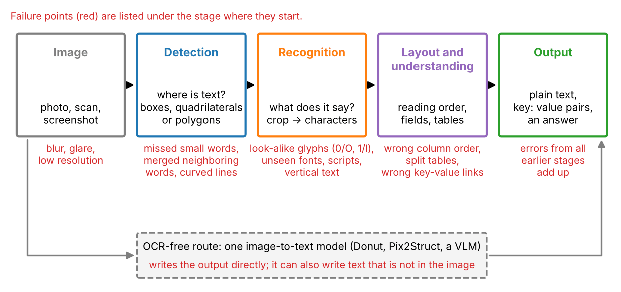
Why a separate chapter? A word is long, thin, often rotated or curved, and packed close to its neighbors; its “class” is not a label from a fixed list but any string over an alphabet that may hold tens of thousands of symbols; and one wrong character can change the meaning (“1046” versus “1O46” on an invoice). The field therefore has its own detectors, sequence recognizers, metrics and benchmarks. It is now being reshaped by models that read a whole page and write structured text directly, which makes the pipeline optional but adds a new risk: fluent output that the image does not support. Figure 1 shows the pipeline and where each stage typically fails.
This chapter assumes DLCV 03 for boxes, IoU, NMS and precision–recall. Other ideas are linked rather than repeated: the CTC algorithm (PR 06’s CTC note), edit distance (PR 06), attention (NLP 07) and vision-language models (ML 10). Surveys by Long et al. [1] and Chen et al. [2] frame scene text; Cui et al. [3] and Zhang et al. [4] cover documents.
The reading pipeline and where it breaks
Plain version. A classical OCR system is a chain: find text regions, read each one, then order the readings and attach meaning. Every link passes its mistakes to the next.
Scene text versus document text
The two settings differ in what is hard.
| Scene text | Document text | |
|---|---|---|
| Source | photos, video, street views | scans, PDFs, screenshots, phone photos of pages |
| Amount | a few words per image | hundreds to thousands of words per page |
| Geometry | any orientation, perspective, curves | mostly horizontal lines; columns, tables |
| Appearance | decorative fonts, clutter, glare, blur | small print, noise, stamps, handwriting |
| Main difficulty | finding and reading each word | reading order, structure and meaning |
Benchmarks follow the split. The Robust Reading competitions held with ICDAR (the International Conference on Document Analysis and Recognition) defined many of the standard scene-text benchmarks: ICDAR 2013 with focused, mostly horizontal English text [5], and ICDAR 2015’s Incidental Scene Text challenge [6], recorded with wearable cameras (Google Glass), where words are often small, blurred and rotated [7]. Document benchmarks ask for layout regions, form fields or answers about a page (Document understanding).
Four places where errors start
Errors are easier to fix when you know which stage produced them.
- Image. Blur, glare, low resolution and compression remove the evidence. No later stage can recover a character that is not in the pixels; a generative model that “recovers” it is guessing (see Failure modes).
- Detection. A missed word is lost for good; two words merged into one box are read as one string; a box that cuts off the last letter produces a deletion.
- Recognition. Look-alike glyphs (0/O, 1/l/I, rn/m), unseen fonts and scripts, and vertical text cause substitutions.
- Layout and understanding. Correct words in the wrong order, a table read across instead of down, or a value attached to the wrong key give a wrong answer from perfect characters.
A useful habit: evaluate each stage on its own (recognition on ground-truth crops, for example) before the whole chain, so you know which stage to improve.
Before deep learning: thresholds and connected components
Plain version. On clean pages, threshold dark pixels, group connected regions and fit boxes. Uneven backgrounds and touching characters expose this baseline’s limits.
The classical recipe has three steps. Binarization labels each pixel as ink or paper by comparing it with a threshold. A single global threshold, for example the one chosen by Otsu’s method [8] (derived in IP 10), fails under uneven lighting, so document systems use a local threshold computed in a window around each pixel. Sauvola’s method [9], designed for document images, is a common choice:
where is the threshold at pixel , and are the mean and standard deviation of the gray levels in a window centered on the pixel, is the dynamic range of the standard deviation, and (scikit-image’s default is 0.2) controls how much local contrast lowers the threshold. A pixel darker than is ink. Grouping then joins ink pixels into connected components (IP 09), usually after a horizontal dilation that bridges the gaps between the letters of a word. Box extraction takes the bounding box of each component.
The snippet renders a small invoice with matplotlib, darkens its left side, adds noise, and runs this recipe with a global and a local threshold. It scores the boxes with the precision, recall and H-mean used by text benchmarks (defined precisely in Measuring OCR): a predicted box counts as correct if its IoU with a still-unmatched ground-truth word is at least 0.5.
Code · Python · 64 lines
import numpy as np
import matplotlib
matplotlib.use("Agg")
import matplotlib.pyplot as plt
from scipy import ndimage as ndi
from skimage.filters import threshold_otsu, threshold_sauvola

H, W = 200, 560
WORDS = [("INVOICE", 20, 18, 22), ("No.", 200, 24, 14), ("1046", 245, 24, 14),
         ("Date:", 330, 24, 14), ("2026-11-01", 385, 24, 14),
         ("Item", 20, 80, 13), ("Qty", 260, 80, 13), ("Price", 400, 80, 13),
         ("Paper", 20, 110, 13), ("12", 265, 110, 13), ("3.50", 405, 110, 13),
         ("Total", 20, 160, 15), ("42.00", 395, 160, 15)]     # (word, x, y, font size)

def render(words):
    """Draw words with matplotlib; return a gray image in [0, 1] and word boxes."""
    fig = plt.figure(figsize=(W / 100, H / 100), dpi=100)
    texts = [fig.text(x / W, 1 - y / H, s, fontsize=fs, va="top") for s, x, y, fs in words]
    fig.canvas.draw()
    img = np.asarray(fig.canvas.buffer_rgba())[..., :3].mean(axis=2) / 255.0
    r = fig.canvas.get_renderer()
    boxes = [[b.x0, H - b.y1, b.x1, H - b.y0]
             for b in (t.get_window_extent(r) for t in texts)]
    plt.close(fig)
    return img, np.array(boxes)

def iou(a, b):
    w = min(a[2], b[2]) - max(a[0], b[0]); h = min(a[3], b[3]) - max(a[1], b[1])
    inter = max(w, 0) * max(h, 0)
    area = lambda r: (r[2] - r[0]) * (r[3] - r[1])
    return inter / (area(a) + area(b) - inter)

def detect(img, thresh, gap=9):
    ink = img < thresh                                   # dark pixels = ink
    ink = ndi.binary_opening(ink, np.ones((2, 2)))       # drop isolated noise pixels
    words = ndi.binary_dilation(ink, np.ones((3, gap)))  # bridge gaps between letters
    lab, _ = ndi.label(words)
    out = []
    for y, x in ndi.find_objects(lab):
        if (y.stop - y.start) * (x.stop - x.start) > 40:   # ignore tiny blobs
            out.append([x.start, y.start, x.stop, y.stop])
    return np.array(out, float)

def h_mean(pred, gt, thr=0.5):
    used, tp = set(), 0
    for p in pred:                                       # greedy one-to-one matching
        cand = [(iou(p, g), j) for j, g in enumerate(gt) if j not in used]
        best = max(cand, default=(0, -1))
        if best[0] >= thr:
            used.add(best[1]); tp += 1
    P, R = tp / max(len(pred), 1), tp / len(gt)
    return P, R, 2 * P * R / max(P + R, 1e-9)

rng = np.random.default_rng(0)
clean, gt = render(WORDS)
shade = 0.45 + 0.55 * np.linspace(0, 1, W)[None, :]      # light falls off to the left
img = np.clip(clean * shade + rng.normal(0, 0.04, clean.shape), 0, 1)

t_sau = threshold_sauvola(img, window_size=31)
for name, t, gap in [("Otsu, gap 9", threshold_otsu(img), 9), ("Sauvola, gap 3", t_sau, 3),
                     ("Sauvola, gap 9", t_sau, 9), ("Sauvola, gap 25", t_sau, 25)]:
    pred = detect(img, t, gap)
    P, R, F = h_mean(pred, gt)
    print(f"{name:16s} boxes={len(pred):2d}  P={P:.2f}  R={R:.2f}  H-mean={F:.2f}")
Output
Otsu, gap 9      boxes= 8  P=0.62  R=0.38  H-mean=0.48
Sauvola, gap 3   boxes=33  P=0.15  R=0.38  H-mean=0.22
Sauvola, gap 9   boxes=13  P=1.00  R=1.00  H-mean=1.00
Sauvola, gap 25  boxes=11  P=0.64  R=0.54  H-mean=0.58
Figure 2 shows what happened. The global threshold marks the whole dark left side as ink, so the words there vanish into one large false box. The local threshold recovers every word, but only for one hand-chosen gap: a narrow dilation splits words into letters, a wide one merges “No.” with “1046” and “Date:” with the date. All numbers here come from this synthetic toy.
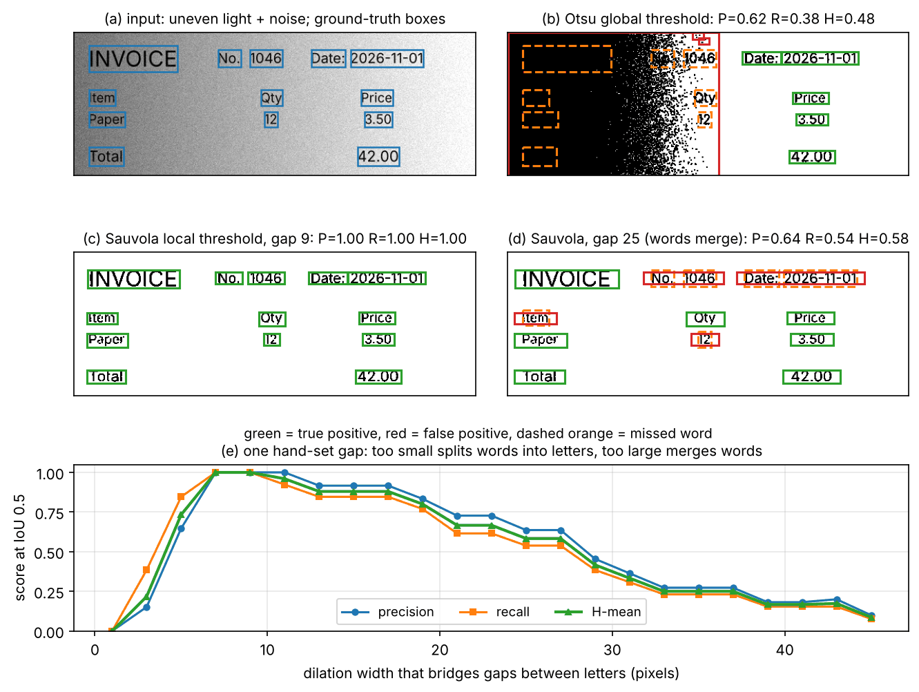
This experiment is the whole motivation for learned text detectors. Real images have every font size at once, text on textured backgrounds, rotation, and words closer together than letters inside other words. A network can learn where text is from context and appearance, and it can learn to keep neighbors apart.
Text detection
Plain version. Text detectors must handle elongated, rotated, curved and closely spaced regions, using geometric predictions or text masks.
Why text is not just another object
The detectors of DLCV 03 predict upright (axis-aligned) boxes. For text this breaks in three ways.
- Extreme aspect ratios. A text line can be many times wider than it is tall, far outside anchor shapes tuned for ordinary objects.
- Orientation and curvature. Words on signs and packages are rotated, seen in perspective, or follow a curve. Benchmarks therefore annotate quadrilaterals (ICDAR 2015 [6]) or polygons (Total-Text [10], CTW1500 [11]), and compute IoU between polygons instead of rectangles.
- Dense neighbors. Words on a line are a few pixels apart; merging them, or letting NMS delete one, loses recall.
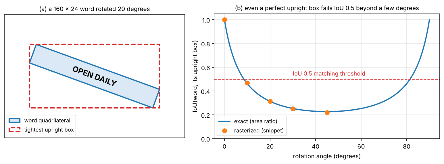
The first two problems combine badly. The snippet computes the IoU between a long thin word and the tightest upright box around it, as the word rotates.
Code · Python · 22 lines
import numpy as np
from skimage.draw import polygon

def rotated_word(cx, cy, w, h, deg):
    """Corners of a w x h word box rotated by deg around its center (x, y)."""
    t = np.deg2rad(deg)
    R = np.array([[np.cos(t), -np.sin(t)], [np.sin(t), np.cos(t)]])
    corners = np.array([[-w, -h], [w, -h], [w, h], [-w, h]]) / 2
    return corners @ R.T + [cx, cy]

def mask(quad, shape=(300, 300)):
    m = np.zeros(shape, bool)
    rr, cc = polygon(quad[:, 1], quad[:, 0], shape)
    m[rr, cc] = True
    return m

for deg in [0, 10, 20, 30, 45]:
    quad = rotated_word(150, 150, 160, 24, deg)          # a long, thin word
    x0, y0 = quad.min(axis=0); x1, y1 = quad.max(axis=0)
    aabb = np.array([[x0, y0], [x1, y0], [x1, y1], [x0, y1]])  # tightest upright box
    a, b = mask(quad), mask(aabb)
    print(f"angle {deg:2d} deg: IoU(word, its upright box) = {(a & b).sum() / (a | b).sum():.2f}")
Output
angle  0 deg: IoU(word, its upright box) = 1.00
angle 10 deg: IoU(word, its upright box) = 0.47
angle 20 deg: IoU(word, its upright box) = 0.31
angle 30 deg: IoU(word, its upright box) = 0.25
angle 45 deg: IoU(word, its upright box) = 0.22
For a rectangle rotated by the exact value is , where and are the word’s width and height and the denominator is the area of its upright bounding box. Already at 10 degrees the best possible upright box fails the usual IoU 0.5 test (Figure 3). Text detectors therefore output rotated rectangles, quadrilaterals or polygons; how IoU is computed for rotated shapes is the same polygon-clipping problem solved for bird’s-eye-view boxes in DLCV 03B.
Regression-based detectors: EAST
Plain version. Each text pixel predicts confidence and word geometry. Merge consistent high-confidence predictions into detections.
EAST (Efficient and Accurate Scene Text detector) [12] is a fully convolutional network with a U-shaped feature-merging branch that outputs, at each location of a downsampled map, a score in (is this pixel inside a shrunk version of a word?) and a geometry. Two geometries were proposed. RBOX has five channels: the distances from the pixel to the four sides of a rotated rectangle and the rectangle’s rotation angle. QUAD has eight channels: the offsets , , from the pixel to the four corners of a quadrilateral. Because tens of thousands of pixels vote, EAST first merges neighboring geometries row by row, averaging them with their scores as weights (locality-aware NMS), and only then runs standard NMS [12]. One network pass replaces the candidate-grouping steps of earlier systems. Its weakness is reach: a pixel must predict edges that may be hundreds of pixels away, and a quadrilateral cannot follow a curved word.
Segmentation-based detectors: PSENet and DBNet
Plain version. Instead of asking each pixel for the whole word’s shape, ask only “is this pixel text?” That gives a mask that can follow any curve. The difficulty is splitting a mask into words when the words touch, so these detectors predict a thinner core for each word, keep the cores apart, and grow them back afterwards.
The network is an encoder–decoder like those of DLCV 04, predicting a per-pixel text probability map ; the trick is in the labels. Each ground-truth polygon with area and perimeter is shrunk inward by an offset
where is a shrink ratio; the shrunk polygon (the word’s kernel) is the positive region. Kernels of adjacent words are separated by a margin even when the words touch, so connected components of the predicted kernel map are word instances; each is then dilated back to full size.
PSENet (Progressive Scale Expansion Network) [13] predicts several kernels per word at different shrink ratios and grows the smallest, well-separated ones into the larger ones with a breadth-first search, so a pixel claimed by one word cannot be taken by its neighbor. The price is a slow, sequential post-process.
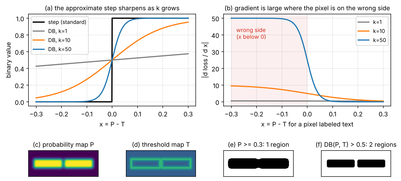
DBNet [14] keeps a single kernel and makes the binarization step itself trainable. A standard binarization with a fixed threshold has zero gradient almost everywhere, so it cannot be trained. DBNet predicts a second map, a threshold map , and uses the approximate step
where is the approximate binary value at pixel , the predicted text probability, the learned threshold and an amplifying factor set to 50 [14]. Writing and , the binary cross-entropy for a text pixel, , has derivative , and for a background pixel, , . The gradient is scaled by and is largest where a pixel is on the wrong side of its threshold. The threshold map is supervised to be high in a band around each word’s border, so the binarization is strict where words meet and relaxed inside them.
The snippet checks the derivative numerically and shows, on a 1-D profile, a threshold that is high between two words separating them where a fixed threshold merges them.
Code · Python · 22 lines
import numpy as np

def db(P, T, k=50.0):
    """Differentiable binarization: an approximate step at the learned threshold T."""
    return 1.0 / (1.0 + np.exp(-k * (P - T)))

x = np.array([-0.10, -0.02, 0.0, 0.02, 0.10])            # x = P - T at five pixels
for k in [1.0, 50.0]:
    f = db(x, 0.0, k)
    g_pos = -k * (1 - f)       # d/dx of -log f       (pixel labeled text)
    g_neg = k * f              # d/dx of -log(1 - f)  (pixel labeled background)
    # check the text-pixel gradient by finite differences
    eps = 1e-6
    num = (-np.log(db(x + eps, 0, k)) + np.log(db(x - eps, 0, k))) / (2 * eps)
    assert np.allclose(num, g_pos, rtol=1e-4)
    print(f"k={k:4.0f}  B_hat={np.round(f, 3)}  dl+/dx={np.round(g_pos, 2)}  dl-/dx={np.round(g_neg, 2)}")

# Two words whose probability map P does not drop to 0 between them.
P = np.array([0.1, 0.9, 0.95, 0.9, 0.55, 0.5, 0.55, 0.9, 0.95, 0.9, 0.1])
T = np.array([0.3, 0.3, 0.3, 0.3, 0.7, 0.7, 0.7, 0.3, 0.3, 0.3, 0.3])   # high at the gap
print("fixed t=0.3:", (P >= 0.3).astype(int))
print("DB, k=50   :", (db(P, T) > 0.5).astype(int))
Output
k=   1  B_hat=[0.475 0.495 0.5   0.505 0.525]  dl+/dx=[-0.52 -0.5  -0.5  -0.5  -0.48]  dl-/dx=[0.48 0.5  0.5  0.5  0.52]
k=  50  B_hat=[0.007 0.269 0.5   0.731 0.993]  dl+/dx=[-49.67 -36.55 -25.   -13.45  -0.33]  dl-/dx=[ 0.33 13.45 25.   36.55 49.67]
fixed t=0.3: [0 1 1 1 1 1 1 1 1 1 0]
DB, k=50   : [0 1 1 1 0 0 0 1 1 1 0]
With the “binary” map is a gray blur near 0.5 and every pixel gets the same small gradient; with it is nearly binary, and a text pixel 0.1 below its threshold gets a gradient of about while a correct one gets almost none. Figure 4 repeats the separation in 2-D.
At inference DBNet drops the threshold branch: it binarizes at a constant 0.2, takes connected components, and expands each region by , with and the region’s area and perimeter and [14]. The threshold map is thus mainly a training device that makes itself sharp, and the simple post-processing keeps the detector fast.
Optional: Shrinking and expanding text polygons (in the Supplementary notes). The shrink offset worked out for rectangles, why it never erases a word, and why one expansion ratio cannot restore every aspect ratio exactly.
Optional: DBNet: a reading guide (in the Paper guides). How the paper’s ablation and benchmark tables are organized and what to check in them.
Character-level and curved-text detectors
Some detectors find letters first and glue neighbors into words. CRAFT [15] predicts a region score (center of a character) and an affinity score (between two characters of one word) and links characters into words of any shape; because real datasets label only words, it estimates character labels on real images with an interim model. Polygon detectors such as the one introduced with CTW1500 [11] instead regress many boundary points along a curved line. Richer shape models follow irregular text better but need more complex outputs or post-processing.
Text recognition
Plain version. Recognition takes one cropped word or line and outputs its characters. The modern approach reads the crop like a sequence: slide along it from left to right, describe each thin slice, and turn the sequence of slices into a sequence of characters, without ever cutting the word into separate letters.
Recognition as sequence prediction
Early systems cut a word into characters and classified each, which fails when letters touch or break. CRNN (Convolutional Recurrent Neural Network) [16] made recognition segmentation-free and end-to-end trainable. A crop is resized to a fixed height; a CNN turns it into a feature map whose columns form a feature sequence, each column describing a thin vertical strip of the image; a deep bidirectional LSTM (see ML 04) adds left and right context; and a transcription layer turns per-column predictions into a label sequence. With rectangular pooling windows, a 100 × 32 input yields a sequence of 25 frames, longer than most English words [16]. Nothing tells the network which frame belongs to which character; CTC handles that missing alignment.
CTC: training without alignments
Plain version. At every frame the network may say a character or “nothing new” (a blank). To read the output, merge repeated characters and delete the blanks. To train, add up the probability of every frame-by-frame story that reads out as the correct word.
Connectionist temporal classification (CTC) [17] defines, for per-frame probabilities of each symbol (a character of the alphabet or the blank ) at frame , a collapsing map (merge repeats, then remove blanks) and the probability of a label sequence given the input ,
where is an alignment (one symbol per frame), the number of frames, and the sum runs over every alignment that collapses to . Training minimizes , computed by a forward recursion in for a label of length . The full derivation, with a brute-force check, is in PR 06’s CTC note; here we only need what it implies for decoding.
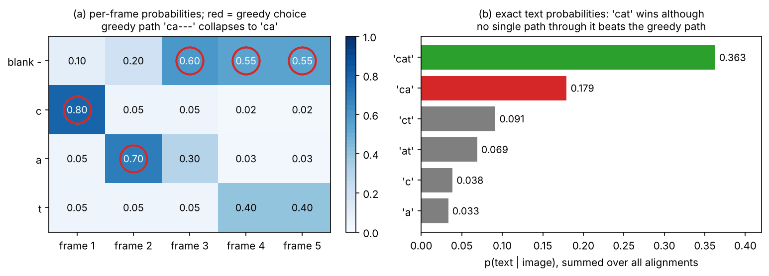
The cheapest decoder is greedy (best-path) decoding: take the most likely symbol at each frame and collapse. CRNN uses exactly this approximation in its lexicon-free mode [16]. But the most likely path need not collapse to the most likely text, because a text’s probability is spread over many paths. The snippet builds a five-frame toy where this matters.
Code · Python · 28 lines
import itertools
import numpy as np

alphabet = ["-", "c", "a", "t"]                 # index 0 is the CTC blank
# Per-frame probabilities from a recognizer (rows: 5 frames, columns: symbols).
probs = np.array([[0.10, 0.80, 0.05, 0.05],
                  [0.20, 0.05, 0.70, 0.05],
                  [0.60, 0.05, 0.30, 0.05],
                  [0.55, 0.02, 0.03, 0.40],
                  [0.55, 0.02, 0.03, 0.40]])

def collapse(path):
    """CTC map B: merge repeated symbols, then remove blanks."""
    merged = [s for i, s in enumerate(path) if i == 0 or s != path[i - 1]]
    return "".join(alphabet[s] for s in merged if s != 0)

greedy = probs.argmax(axis=1)                   # best symbol at every frame
print("greedy path:", "".join(alphabet[s] for s in greedy), "->", repr(collapse(greedy)))

# Exact: add up every alignment that collapses to the same text (4**5 = 1024 paths).
total = {}
for path in itertools.product(range(4), repeat=len(probs)):
    p = np.prod(probs[np.arange(len(probs)), path])
    total[collapse(path)] = total.get(collapse(path), 0.0) + p
for text, p in sorted(total.items(), key=lambda kv: -kv[1])[:3]:
    print(f"p({text!r}) = {p:.3f}")
print("collapse('caa-at') =", repr(collapse([1, 2, 2, 0, 2, 3])),
      " collapse('caaat') =", repr(collapse([1, 2, 2, 2, 3])))
Output
greedy path: ca--- -> 'ca'
p('cat') = 0.363
p('ca') = 0.179
p('ct') = 0.091
collapse('caa-at') = 'caat'  collapse('caaat') = 'cat'
The “t” is never the single most likely symbol in any frame, so greedy decoding drops it, yet the alignments that contain a “t” in frame 4 or 5 add up to twice the probability of “ca” (Figure 5). The last line shows the blank’s second job: a doubled letter survives only with a blank between its copies. Real decoders use prefix beam search, which keeps the best few partial transcriptions and merges alignments that collapse to the same prefix.
Optional: CTC prefix beam search, step by step (in the Supplementary notes). The two probabilities each prefix keeps, the three update rules, and a tested implementation that finds ‘cat’ on this toy.
CTC has two built-in limits (see PR 06’s note): frame outputs are independent given the image, so the model cannot condition on characters it has already emitted, and the alignment is monotonic, so reading order must match frame order. Vertical or curved text breaks the second unless it is rectified first.
Attention decoders and rectification
Plain version. An attention decoder writes the word one character at a time. Before each character it looks back at the image features and chooses where to look; it also remembers what it has already written, so it behaves like a small language model of spelling.
An attention decoder is the encoder–decoder of NLP 07 applied to image features: at step it attends to the feature sequence and predicts character from the result and from , until an end token. It drops CTC’s independence assumption at the price of sequential decoding. ASTER [18] pairs such a decoder with a rectification network: a thin-plate spline (TPS) transformation, predicted from the image and trained only through the recognition loss, warps a curved or perspective word into a straight horizontal one before reading it.
Baek et al. [7] showed that most recognizers of the time fit one four-stage template — transformation (none or TPS), feature extraction, sequence modeling (none or BiLSTM) and prediction (CTC or attention) — and, retraining all combinations on the same data, that attention mainly costs speed and that earlier comparisons had been distorted by different training sets and test subsets.
Optional: Baek et al., “What Is Wrong With Scene Text Recognition Model Comparisons?” (in the Paper guides). The four-stage framework, the dataset audit and how to read the trade-off plots.
Transformer recognizers
TrOCR [19] replaces both the CNN and the RNN with pre-trained transformers. The image is resized to 384 × 384 and split into 16 × 16 patches, as in a Vision Transformer (ML 05); an image encoder initialized from DeiT or BEiT encodes the patches, and a text decoder initialized from RoBERTa or MiniLM generates wordpieces (subword tokens) autoregressively, decoded with beam search [19]. It is pre-trained on synthetic text images and fine-tuned on printed, handwritten and scene text: recognition now borrows its backbones and decoder from general vision and language pre-training.
PARSeq [20] trains one transformer decoder on many random orders of the output positions (permutation language modeling), so the same weights can decode left to right, decode all characters in parallel without context, or refine a first guess using context on both sides.
Language models: help and harm
A recognizer that “knows English” can fix a smudged letter: “PLEA_E” is almost certainly “PLEASE”. The knowledge can be implicit (an autoregressive decoder conditions on its previous characters), a lexicon (CRNN can restrict the output to a word list [16]) or an explicit language model: in ABINet [21] a separate bidirectional language model iteratively corrects the vision model’s output.
The same prior can hurt. Text that is not language — serial numbers, codes, prices, names, mixed scripts — is exactly where OCR matters most and where a language model “corrects” correct readings. PARSeq’s authors note this risk for external language models that do not see the image [20], and OCRBench reports that large multimodal models are weak on non-semantic text (random character strings) as well as on handwriting, multilingual text and mathematical expressions [22]. When the content is not natural language, measure with and without the language prior.
Optional: Where the language model sits in a recognizer (in the Supplementary notes). Lexicon search, implicit and explicit language models, and how to test whether a prior is over-correcting.
Training data: synthetic text
Labeled real crops are scarce, and recognizers trained only on synthetic text generalize well across scene-text datasets [1]. MJSynth [23] renders single words with varied fonts, shadows, distortions and noise (8.9 million word images); SynthText [24] pastes text into natural photos following the scene geometry (5.5 million cropped words) [7]. Training on both beats either alone, and a combined 20% sample of each beats either full set, so diversity can matter more than size [7].
End-to-end text spotting
Plain version. Instead of running a detector and then a separate recognizer on each crop, one network does both and shares its features. Reading helps finding (a region that reads as a word is probably text), and finding helps reading.
A text spotter outputs (shape, transcription) pairs directly. FOTS [25] shares convolutional features between a dense per-pixel detection branch and a recognition branch decoded with CTC, through RoIRotate, an operator that crops and rotates the feature region of each detected quadrilateral into an upright, fixed-height strip. Mask TextSpotter [26] extends Mask R-CNN (see instance segmentation in DLCV 04) with masks for whole words and for individual characters, so it can read curved text without a sequence model. ABCNet [27] fits each curved text instance with parametric Bézier curves and samples features along them with BezierAlign, a curved analogue of RoIAlign. End-to-end evaluation then asks whether each ground-truth word was both located and read correctly, which we define in Measuring OCR.
Document understanding
Plain version. On a page, reading the words is often the easy part. The questions are which words belong together, in which order to read them, and what they mean: which number is the total, which line is the title, which cell is in which column.
Layout analysis and reading order
Layout analysis finds the regions of a page — paragraphs, titles, lists, tables, figures — usually by object detection or instance segmentation on page images. PubLayNet [28] matched the XML and PDF versions of over a million PubMed Central articles to label over 360 thousand page images automatically with five classes (text, title, list, table, figure). DocLayNet [29] has 80,863 manually annotated pages from diverse sources with 11 classes, in COCO format, because models trained only on scientific articles transfer poorly to reports, manuals and forms.
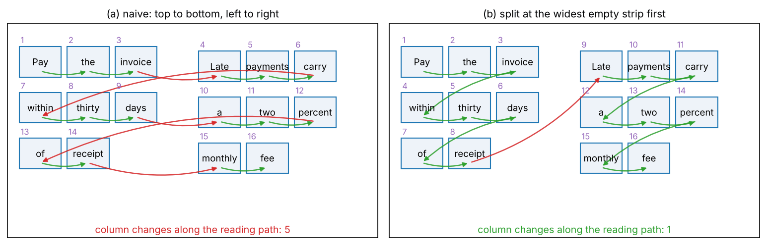
Given regions and words, the system must also produce a reading order. The obvious rule, “top to bottom, then left to right”, fails on the simplest multi-column page, as the snippet shows on a two-column notice.
Code · Python · 35 lines
import numpy as np

# Word boxes (x0, y0, x1, y1) on a two-column page: each column is one sentence.
left = "Pay the invoice within thirty days of receipt".split()
right = "Late payments carry a two percent monthly fee".split()
words, boxes = [], []
for col, text in [(0, left), (1, right)]:
    for k, w in enumerate(text):
        row, pos = divmod(k, 3)                       # three words per line
        x0 = 40 + 300 * col + 80 * pos
        y0 = 100 + 30 * row + 3 * col                 # columns not perfectly aligned
        words.append(w); boxes.append([x0, y0, x0 + 70, y0 + 20])
boxes = np.array(boxes, float)

def naive_order(boxes, line_tol=10):
    """Top-to-bottom, then left-to-right, treating boxes within line_tol as one line."""
    line = np.round(boxes[:, 1] / line_tol)
    return np.lexsort((boxes[:, 0], line))

def column_order(boxes, line_tol=10):
    """Split the page at the widest empty vertical strip, then read column by column."""
    x_min, x_max = int(boxes[:, 0].min()), int(boxes[:, 2].max())
    covered = np.zeros(x_max - x_min, bool)
    for x0, _, x1, _ in boxes.astype(int):
        covered[x0 - x_min:x1 - x_min] = True
    edges = np.flatnonzero(np.diff(np.r_[1, covered.astype(int), 1]))  # empty-run bounds
    starts, ends = edges[::2], edges[1::2]
    widest = np.argmax(ends - starts)
    split = x_min + (starts[widest] + ends[widest]) / 2
    col = (boxes[:, 0] > split).astype(int)
    line = np.round(boxes[:, 1] / line_tol)
    return np.lexsort((boxes[:, 0], line, col))

print("naive :", " ".join(words[i] for i in naive_order(boxes)))
print("column:", " ".join(words[i] for i in column_order(boxes)))
Output
naive : Pay the invoice Late payments carry within thirty days a two percent of receipt monthly fee
column: Pay the invoice within thirty days of receipt Late payments carry a two percent monthly fee
Every word in the naive output is correct, and the text is still useless. The column rule fixes this page but is another hand-made rule that fails on tables or figures (Figure 6); learned layout and document models exist largely to replace such rules.
Text plus layout: the LayoutLM family
Plain version. Give a language model not only the words of a page but also where each word sits. Then “Total” followed by a number at the bottom right of a receipt means something different from the same word in the middle of a paragraph.
LayoutLM [30] starts from BERT (NLP 10) and adds a 2-D position embedding to each word’s token embedding. Each word comes with its OCR box — upper-left and lower-right corners — rescaled to integer “virtual” coordinates from 0 to 1,000 so that pages of different sizes share one scale. Four embedding lookups are added, with one table shared by and and another by and :
where is the input vector of the -th word , and are BERT’s token and 1-D position embeddings, and , are the learned tables for horizontal and vertical coordinates. Pre-training masks some words but keeps their 2-D positions, and the model predicts them from text and layout context (a masked visual-language model), on about 11 million scanned pages OCRed with the open-source Tesseract engine [30], [31]. LayoutLM also adds visual features of each word’s image region, computed with a Faster R-CNN model, for downstream tasks [30]. LayoutLMv3 [32] instead feeds the page image as patches, masks both text tokens and image patches and adds a word–patch alignment objective, so one model serves text-centric tasks (forms, receipts, question answering) and image-centric ones (document classification, layout analysis).
Key information extraction — pulling “invoice number”, “date” and “total” out of a page — is then token classification over the OCR words, as in NLP 06’s sequence labeling, plus linking keys to values. FUNSD [33] is a small benchmark of this kind: 199 real, noisy scanned forms whose semantic entities are labeled question, answer, header or other, with links between them.
The family’s weakness is its input: it cannot fix a word the OCR engine missed or misread, and it inherits the engine’s reading order.
OCR-free models: Donut and Pix2Struct
Plain version. Skip the OCR engine. Train one model to look at the page image and write the desired output — the full text, a JSON record, or an answer — token by token, the way an image captioner writes a caption.
Donut (Document understanding transformer) [34] is a Swin Transformer encoder (ML 05) and a BART decoder. It is pre-trained to read all the text of a page in reading order — a “pseudo-OCR” task on 11 million scanned English documents plus synthetic pages in Chinese, Japanese, Korean and English from its SynthDoG generator — and fine-tuned to emit a token sequence that converts one-to-one into JSON, for classification, information extraction or question answering [34]. It avoids the cost of running OCR, the inflexibility of OCR engines across languages and document types, and the propagation of OCR errors. Pix2Struct [35] is pre-trained to parse masked screenshots of web pages into simplified HTML, which mixes OCR, language modeling and captioning in one objective; it accepts variable-resolution inputs and renders the question directly onto the image.
The price is resolution and verifiability. Donut uses 2560 × 1920 inputs and reports that accuracy rises quickly with input size on documents with tiny text, at a growing compute cost [34]; and because the model generates rather than transcribes, nothing ties each output character to a region of the image.
Optional: Donut: a reading guide (in the Paper guides). The two training stages, the JSON output format, the TED-based accuracy, and the resolution analysis.
Vision-language models for documents
General multimodal large language models (ML 10) now answer questions about documents and transcribe pages; reading small text depends on tiling or dynamic resolution (What the diagram hides). Three cautions apply. First, a fluent answer is not a transcription: check it against detections or ask for coordinates and verify them. Second, generative readers have their own failure modes: the academic-document model Nougat [36] reports that it sometimes degenerates into repeating a sentence over and over (on 1.5% of its test pages, more often out of domain), and that numbers in reference lists and section titles are sometimes skipped or hallucinated. Third, measure the specific skill: OCRBench [22] gathers 29 datasets to test text recognition, scene-text and document question answering, key information extraction and handwritten mathematical expressions separately, instead of hiding OCR inside one aggregate score.
Handwriting, many scripts and CJK text
Plain version. Handwriting varies from writer to writer and joins letters together; many scripts have far more symbols than the Latin alphabet; and some, such as Chinese, can also be written vertically. Each of these breaks an assumption that English scene-text models make quietly.
Handwriting
Offline handwriting recognition reads lines of handwritten text from scans. The IAM database [37] of handwritten English sentences is, in the TrOCR authors’ words, the most popular dataset for handwritten text recognition; TrOCR uses a split of 6,161 training, 966 validation and 2,915 test lines and reports case-sensitive CER [19]. Line-level recognizers with CTC or attention apply unchanged; the difficulty is variation between writers, connected letters and limited labeled data, which is why synthetic pre-training and large pre-trained decoders help. For Chinese handwriting, the CASIA online and offline databases [38] provide data for both pen-trajectory (online) and scanned (offline) recognition.
Large character sets and vertical text
Chinese and Japanese use alphabets of tens of thousands of symbols, against a few dozen for Latin script [1]. RCTW-17 lists what makes Chinese text different: a much larger character set, no spaces between words, and many characters made of several unconnected parts [39]. Each has a consequence. The recognizer’s output layer grows with the alphabet and most characters are rare: the Chinese Text in the Wild dataset labels 1,018,402 character instances in 32,285 street-view images, covering 3,850 distinct characters, most of them rarely used [40]. Unconnected parts break connected-component grouping. And without spaces, systems work on lines and characters rather than words (see NLP 01).
Vertical text is the other difficulty: Chinese can be set vertically as well as horizontally, and street-view datasets such as CTW contain vertical text [40]. The W3C’s Requirements for Chinese Text Layout describes vertical composition: characters run from top to bottom and lines from right to left, while embedded Latin words are either set upright or rotated 90° clockwise [41]. A recognizer that assumes left-to-right frames on a horizontal crop reads such a column as garbage; Baek et al. list vertical text among the failure cases common to all 24 recognizers they tested [7]. The remedy is to decide each detected line’s orientation first and rotate or rearrange it before reading.
Optional: Reading vertical and mixed-direction text (in the Supplementary notes). The layout rules that matter for OCR, how orientation is decided per line, and what a crop must look like before a horizontal recognizer can read it.
Many scripts at once
Multilingual systems must also decide which script they are looking at. The ICDAR 2019 multi-lingual challenge (MLT-2019) [42] has 20,000 real images with text in 10 languages, and includes a script-identification task; its languages cover seven scripts [2].
Measuring OCR
Plain version. Count mistakes the way a proofreader would: how many characters must be inserted, deleted or changed to turn the output into the truth. For detection, count how many found boxes are right and how many real words were found, as in object detection.
CER and WER from edit distance
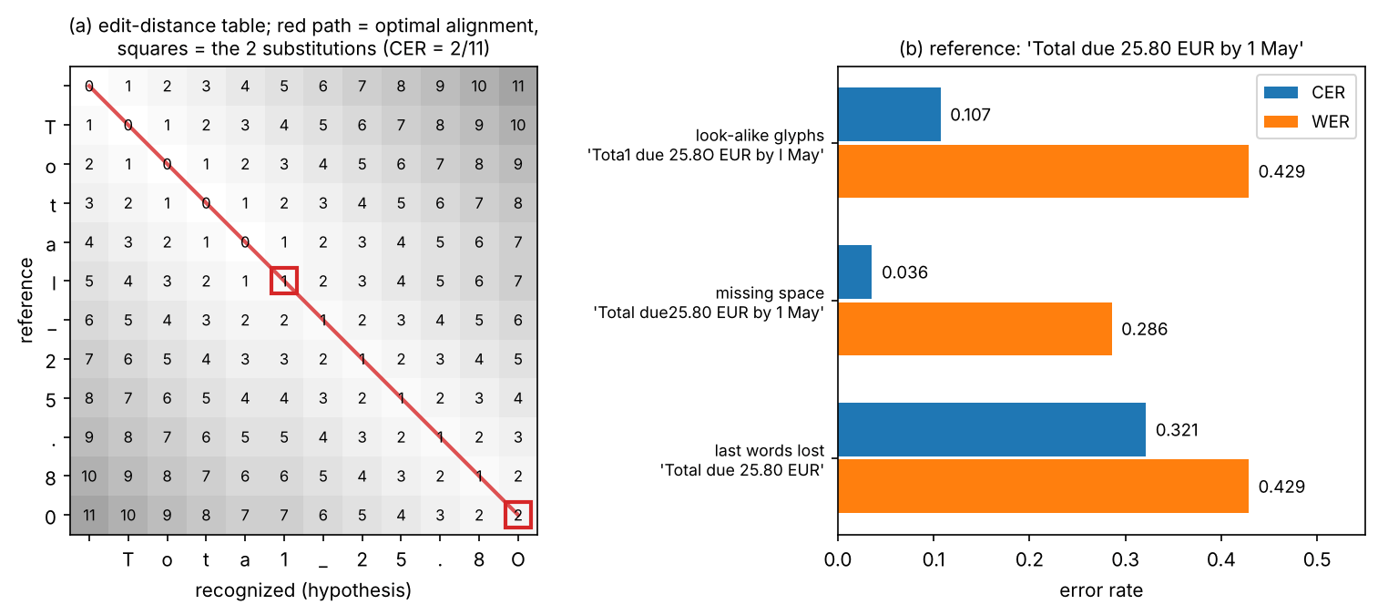
The edit distance (Levenshtein distance) between a reference string and a recognized string is the minimum number of insertions, deletions and substitutions that turn one into the other; the Wagner–Fischer dynamic program computes it [43] (derived in PR 06). Following an optimal alignment back through the table splits the total into substitutions, deletions and insertions. Then
where is the number of characters in the reference, and , , and are the same quantities counted over words (sequences split at spaces). Both are error rates: 0 is perfect, and they can exceed 1 when the output contains many insertions. Other conventions exist: scene-text recognition on cropped words usually reports word accuracy (the fraction of crops read exactly), some papers call one minus that the word error rate, and multilingual competitions report one minus a normalized edit distance (NED) [2]. Always state which one you report.
Code · Python · 34 lines
import numpy as np

def edit_ops(ref, hyp):
    """Levenshtein alignment of two sequences; returns (S, D, I) counts."""
    n, m = len(ref), len(hyp)
    E = np.zeros((n + 1, m + 1), int)
    E[:, 0], E[0, :] = np.arange(n + 1), np.arange(m + 1)
    for i in range(1, n + 1):
        for j in range(1, m + 1):
            E[i, j] = min(E[i - 1, j] + 1, E[i, j - 1] + 1,
                          E[i - 1, j - 1] + (ref[i - 1] != hyp[j - 1]))
    S = D = I = 0
    i, j = n, m
    while i > 0 or j > 0:                       # walk back along one optimal path
        if i > 0 and j > 0 and E[i, j] == E[i - 1, j - 1] + (ref[i - 1] != hyp[j - 1]):
            S += ref[i - 1] != hyp[j - 1]; i, j = i - 1, j - 1
        elif i > 0 and E[i, j] == E[i - 1, j] + 1:
            D += 1; i -= 1
        else:
            I += 1; j -= 1
    return S, D, I

def rates(ref, hyp):
    c = edit_ops(ref, hyp)
    w = edit_ops(ref.split(), hyp.split())
    return c, sum(c) / len(ref), w, sum(w) / len(ref.split())

ref = "Total due 25.80 EUR by 1 May"
for hyp in ["Total due 25.80 EUR by 1 May",
            "Tota1 due 25.8O EUR by l May",      # three look-alike glyphs
            "Total due25.80 EUR by 1 May",       # one missing space
            "Total due 25.80 EUR"]:              # last words not read
    c, cer, w, wer = rates(ref, hyp)
    print(f"{hyp:30s} chars S,D,I={c} CER={cer:.3f} | words S,D,I={w} WER={wer:.3f}")
Output
Total due 25.80 EUR by 1 May   chars S,D,I=(0, 0, 0) CER=0.000 | words S,D,I=(0, 0, 0) WER=0.000
Tota1 due 25.8O EUR by l May   chars S,D,I=(3, 0, 0) CER=0.107 | words S,D,I=(3, 0, 0) WER=0.429
Total due25.80 EUR by 1 May    chars S,D,I=(0, 1, 0) CER=0.036 | words S,D,I=(1, 1, 0) WER=0.286
Total due 25.80 EUR            chars S,D,I=(0, 9, 0) CER=0.321 | words S,D,I=(0, 3, 0) WER=0.429
Three look-alike substitutions cost 3 of 28 characters (CER 0.107) but ruin 3 of 7 words (WER 0.429), and one turns an amount into a non-number. One missing space costs one character but two word errors; losing the last three words costs nine characters, spaces included. CER says how much must be fixed; WER, or better a task check such as “is the total correct?”, says whether the output is usable (Figure 7).
Detection: precision, recall and H-mean at IoU 0.5
Text detection uses the precision and recall of DLCV 03 with one matching rule and one summary number. In the protocol used by the Robust Reading competitions, as described for MLT-2019, a detection is a true positive if its IoU with a ground-truth quadrilateral exceeds 0.5, each ground truth and each detection may be matched at most once, and detections that overlap a region marked “do not care” (illegible or out-of-scope text) by more than half of that region’s area are removed before matching [42]. Counts are accumulated over the whole test set, and
where TP is the number of matched pairs, the number of detections after filtering, the number of ground-truth words that are not “do not care”, and the H-mean (harmonic mean of precision and recall, the F-score). Unlike COCO AP, H-mean is a single point of the precision–recall curve, at a confidence threshold chosen by the submitter; Long et al. recommend also reporting AP [1]. ICDAR 2013 used a different, overlap-based protocol, so its numbers are not comparable with IoU-based ones [1].
End-to-end and document metrics
End-to-end spotting first matches detections to ground truth as above and then compares the transcriptions, either for every word (end-to-end recognition) or only for words in a given vocabulary (word spotting); results depend strongly on the size of that vocabulary [2]. Document benchmarks use task metrics: ANLS (average normalized Levenshtein similarity), an edit-distance-based score for DocVQA answers, chosen so that small OCR slips are not scored as total failures [44]; field-level F1 and a tree-edit-distance accuracy for extracted JSON records [34]; and COCO-style mAP for layout regions [29].
Optional: Evaluation protocols in detail (in the Supplementary notes). “Do not care” filtering, one-to-many matching in the ICDAR 2013 protocol, vocabularies, NED and AED, ANLS and TED accuracy, with their edge cases.
Datasets and benchmarks
The table lists the benchmarks named in this chapter. Sizes are as stated in the cited papers.
| Benchmark | Task | Content |
|---|---|---|
| ICDAR 2013 [5] | detection, recognition, end-to-end | focused scene text, mostly horizontal English; 462 images [10] |
| ICDAR 2015 Incidental [6] | detection, recognition, end-to-end | wearable-camera images; 1,000 train / 500 test for detection [12]; quadrilateral labels |
| Total-Text [10] | detection, spotting | 1,555 images (1,255 / 300), 9,330 words, polygons; horizontal, multi-oriented and curved |
| CTW1500 [11] | curved-text detection | 1,500 images (1,000 / 500), over 10,000 text annotations as polygons |
| IIIT5K [45] | cropped-word recognition | words from web image search; 2,000 train / 3,000 test [7] |
| SVT [46] | cropped-word recognition | Google Street View; 257 train / 647 test words [7] |
| MLT-2019 [42] | multilingual detection, script ID, end-to-end | 20,000 images, 10 languages |
| RCTW-17 [39], CTW [40] | Chinese detection and recognition | 12,263 images; 32,285 images with character-level labels |
| IAM [37], CASIA-HWDB [38] | handwriting | English sentences; Chinese online and offline handwriting |
| FUNSD [33] | form understanding | 199 scanned forms; question / answer / header / other entities with links |
| PubLayNet [28], DocLayNet [29] | layout analysis | over 360k auto-labeled article pages (5 classes); 80,863 hand-labeled pages (11 classes) |
| DocVQA [44] | document question answering | 50,000 questions on over 12,000 document images; ANLS |
| OCRBench [22], OmniDocBench [47] | OCR skills of multimodal models; page parsing | 29 datasets; 9 document sources, 19 layout categories |
Two cautions apply to all of them. Different papers have evaluated on different subsets of the same benchmark (Baek et al. found two versions each of IC03 and IC15 in use), so check the subset before comparing numbers [7]. And the labels are not perfect: Baek et al. estimated the mislabeling rate of the common recognition benchmarks at 1.3% ignoring special characters, rising to 6.1% when special characters count and 24.1% when case counts [7].
Failure modes
Plain version. OCR fails where the pixels stop carrying the answer, where the shape or script differs from training, and where a model fills a gap with something plausible. The last kind is the most dangerous, because the output looks perfect.
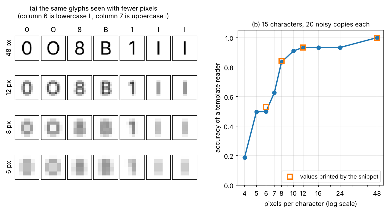
Look-alike glyphs and low resolution. Many characters differ by a few pixels: 0 and O, 1, l and I, 5 and S, 8 and B, “rn” and “m”. The snippet makes a tiny template reader for 15 characters and shows how it degrades as the number of pixels per character drops.
Code · Python · 37 lines
import numpy as np
import matplotlib
matplotlib.use("Agg")
import matplotlib.pyplot as plt
from skimage.transform import resize

CHARS = "0O8B5S1lIZ2aekx"

def glyph(c):
    """Render one character (ink = 1, paper = 0) on a 48 x 48 canvas."""
    fig = plt.figure(figsize=(0.48, 0.48), dpi=100)
    fig.text(0.5, 0.5, c, fontsize=26, ha="center", va="center")
    fig.canvas.draw()
    img = 1 - np.asarray(fig.canvas.buffer_rgba())[..., :3].mean(axis=2) / 255.0
    plt.close(fig)
    return img

def ncc(a, b):
    a, b = a - a.mean(), b - b.mean()
    return (a * b).sum() / np.sqrt((a * a).sum() * (b * b).sum())

templates = {c: glyph(c) for c in CHARS}
rng = np.random.default_rng(0)
for h in [48, 12, 8, 6]:                          # pixels per character cell
    errors, total = {}, 0
    for c, img in templates.items():
        for _ in range(20):
            low = resize(img, (h, h), anti_aliasing=True)       # camera sees few pixels
            low = low + rng.normal(0, 0.05, low.shape)          # sensor noise
            back = resize(low, (48, 48), order=1)               # what the reader gets
            guess = max(CHARS, key=lambda t: ncc(back, templates[t]))
            total += 1
            if guess != c:
                errors[(c, guess)] = errors.get((c, guess), 0) + 1
    top = sorted(errors.items(), key=lambda kv: -kv[1])[:3]
    print(f"{h:2d}px  accuracy={1 - sum(errors.values()) / total:.2f}  most confused: "
          + ", ".join(f"{a}->{b} ({n})" for (a, b), n in top))
Output
48px  accuracy=1.00  most confused:
12px  accuracy=0.93  most confused: l->I (20)
 8px  accuracy=0.84  most confused: I->1 (13), l->1 (12), 0->O (6)
 6px  accuracy=0.53  most confused: B->8 (20), 0->8 (15), S->8 (12)
Lowercase “l” and capital “I” are confused already at 12 pixels, because this sans-serif font draws both as a plain bar (Figure 8); at 6 pixels half the readings are wrong. A deep recognizer does far better than template matching, but no recognizer can separate glyphs that the font draws identically; only context can. Super-resolution can help (DLCV 09A), but see the last item below.
Other common failures, each with the stage where it starts (Figure 1):
- Curved, rotated and perspective text (detection and recognition): upright boxes miss it (Figure 3); horizontal recognizers misread it unless it is rectified.
- Unusual fonts and styles (recognition): calligraphic brand names and shop signs were among the cases that all 24 models in Baek et al.’s study failed on, along with vertical text, special characters, heavy occlusion and low resolution [7].
- Merged or split instances (detection): Figure 2’s gap trade-off in learned form; segmentation detectors fight it with shrunk kernels and learned thresholds.
- Wrong layout (understanding): correct words in the wrong order (Figure 6), tables read across rows, a value linked to the wrong key.
- Distribution shift (all stages): layout models trained only on article pages degrade on more diverse documents [29]; DLCV 14 treats shift in general.
- Hallucinated text (any generative stage): a generative reader can output text that is not in the image — repeated sentences, invented section numbers [36], a “corrected” serial number. The same happens upstream: a generative restoration or super-resolution model can turn unreadable letters into clean, legible, wrong ones, as discussed in DLCV 09B; and text in generated images is often misspelled (DLCV 12). Never run OCR on a generatively enhanced image for anything that must be true, such as an amount, a name or a license plate, without checking against the original.
Modern view
What the surveys say
Four reviews cover this chapter’s ground. Long et al. [1] organize scene-text detection by how much of a word each prediction covers (whole words versus characters, segments or kernels) and recognition into CTC-based and encoder–decoder methods; they see generalization across datasets and large alphabets as the open problems. Chen et al. [2] focus on recognition, organized by pipeline stage, and collect the datasets and evaluation protocols. Cui et al. [3] review document tasks from rule-based analysis to pre-trained LayoutLM-style models, and Zhang et al. [4] split document parsing into modular pipelines and unified VLM-based models, naming complex layouts, the reliability of VLM parsing and inference cost as the main challenges. OCRBench [22] complements them with an evaluation of large multimodal models on text-related tasks.
Optional: Guide to the Modern view surveys (in the Paper guides). What each review covers, how it organizes the field and what it concludes.
The state of the art, 2023–2026
- Pipelines remain the natural choice when coordinates, speed or auditability matter: a DBNet-style detector, an attention or transformer recognizer and a layout model, each evaluated and corrected separately.
- End-to-end page readers are maturing fast. Models that turn a page into Markdown or structured text in one pass now cover formulas, tables and charts: Nougat for academic papers [36]; GOT, which treats plain text, formulas, tables, charts and sheet music as “characters” for one encoder–decoder model [48]; olmOCR, a fine-tuned vision-language model for linearizing PDFs at scale, released with its own benchmark of hard pages [49]; and DeepSeek-OCR, which studies how few vision tokens a page can be compressed into while remaining readable [50]. All of these reports come from their authors.
- Evaluation is catching up. OmniDocBench [47] (CVPR 2025) evaluates pipelines and end-to-end models on pages from nine document sources with 19 layout categories and 15 attribute labels, so that results can be broken down by document type and difficulty instead of one score.
Open problems
- Faithfulness. Generative readers can produce text that is not on the page, and their errors look like correct text. Character-level grounding (which pixels support each output token) and calibrated confidence are not yet standard.
- Non-semantic and rare text. Codes, numbers, names, rare characters in large alphabets and mixed scripts are where language priors help least and errors cost most [22].
- Layout and reading order on complex pages — multi-column articles with floating figures, nested tables, forms with handwritten entries — remain hard for pipelines and end-to-end models alike; robustness to complex layouts is among the main challenges named by Zhang et al. [4].
- Generalization across domains and scripts, including vertical and curved text, without collecting new labels for each domain [1].
- Comparable evaluation. Different subsets, metrics (CER, word accuracy, NED, ANLS) and output normalizations make published numbers hard to compare [7].
Key takeaways
- Evaluate each reading stage and the complete pipeline; upstream errors propagate.
- Rotated, curved and crowded text needs geometry that ordinary upright boxes may not capture.
- Shrunk text regions help separate touching instances; thresholding and region expansion affect the final detections.
- Recognition is sequence prediction; decoding and language priors can help words but distort codes or numbers.
- Layout and OCR-free models change the error pathway, while resolution limits and hallucinated text remain concerns.
- State CER/WER variants, detection matching rules, ignored regions and downstream task metrics.
Exercises
- Gap and font size. In the detection snippet, scale every font size in
WORDSby 0.6 and then by 1.6, and rerun the sweep over the dilation gap. How does the best gap move, and what does that tell you about one fixed post-processing rule for an image that contains both sizes?
Hint
The best gap scales with letter spacing, hence with font size, so an image with both sizes has no single good gap. Learned detectors avoid the problem by predicting word regions, or shrunk kernels, directly.
- Upright boxes by hand. Show that the IoU between a rectangle rotated by and its tightest upright box is . For and , find the angle at which it drops to 0.5, and compare with a square word ().
Hint
The rotated rectangle lies inside its upright box, so the intersection is and the union is the box area. Solving numerically for gives about 8.5°. For a square, the minimum at 45° is exactly, so a square never falls below 0.5: the problem is specific to elongated shapes such as text lines.
- Greedy versus exact CTC. Change the last two rows of the CTC matrix so that the blank and “t” have probabilities 0.65 and 0.30 in both frames. Is “cat” still the most probable text? Then let the “t” probability in frames 4 and 5 run from 0.05 to 0.45, with the blank taking . For which values do greedy and exact decoding agree?
Hint
Reuse the brute-force loop. At , “cat” (about 0.294) still beats “ca” (about 0.249). Greedy decoding returns “ca” until exceeds the blank (above 0.475), but the exact answer switches to “cat” already at ; between those values the two disagree. Below the crossover they agree on “ca”.
- CER that hides a disaster. Construct a reference of 40 characters and two recognitions with the same CER of 0.05 such that one is harmless for an invoice-processing system and the other is fatal. Propose a field-level metric that separates them.
Hint
Two errors in a long description word (“Paper A4 recyled”) versus two errors in the total (“42.00” read as “4Z.0O”). A field-level exact match on the key fields (invoice number, date, total), or the F1 over extracted fields that Donut reports, distinguishes them; CER and WER weight every character or word equally.
- Reading order breaks again. Add a heading “PAYMENT TERMS” that spans both columns above the two-column notice of the reading-order snippet. What does
column_orderproduce? Modify it so that full-width lines are read first, and describe a layout that still defeats your rule.
Hint
The heading crosses the split and is assigned to the left column by its left edge, which happens to work at the top but not for a full-width line in the middle. Treat boxes that overlap the split as a separate band and read band by band. A table, or a figure inside one column, still breaks rules based on empty strips.
References
- S. Long, X. He and C. Yao, “Scene text detection and recognition: The deep learning era,” International Journal of Computer Vision, vol. 129, pp. 161–184, 2021. doi
- X. Chen, L. Jin, Y. Zhu, C. Luo and T. Wang, “Text recognition in the wild: A survey,” ACM Computing Surveys, vol. 54, no. 2, 2021. doi
- L. Cui, Y. Xu, T. Lv and F. Wei, “Document AI: Benchmarks, models and applications,” arXiv:2111.08609, 2021. arXiv
- Q. Zhang, B. Wang, V. S.-J. Huang, J. Zhang, Z. Wang, H. Liang, C. He and W. Zhang, “Document parsing unveiled: Techniques, challenges, and prospects for structured information extraction,” arXiv:2410.21169, 2024. arXiv
- D. Karatzas, F. Shafait, S. Uchida, M. Iwamura, L. Gomez i Bigorda, S. Robles Mestre, J. Mas et al., “ICDAR 2013 Robust Reading Competition,” in Proc. International Conference on Document Analysis and Recognition (ICDAR), pp. 1484–1493, 2013. doi
- D. Karatzas, L. Gomez-Bigorda, A. Nicolaou, S. Ghosh, A. Bagdanov, M. Iwamura, J. Matas et al., “ICDAR 2015 competition on Robust Reading,” in Proc. International Conference on Document Analysis and Recognition (ICDAR), pp. 1156–1160, 2015. doi
- J. Baek, G. Kim, J. Lee, S. Park, D. Han, S. Yun, S. J. Oh and H. Lee, “What is wrong with scene text recognition model comparisons? Dataset and model analysis,” in Proc. IEEE/CVF ICCV, pp. 4714–4722, 2019. doi
- N. Otsu, “A threshold selection method from gray-level histograms,” IEEE Transactions on Systems, Man, and Cybernetics, vol. 9, no. 1, pp. 62–66, 1979. doi
- J. Sauvola and M. Pietikäinen, “Adaptive document image binarization,” Pattern Recognition, vol. 33, no. 2, pp. 225–236, 2000. doi
- C. K. Ch’ng and C. S. Chan, “Total-Text: A comprehensive dataset for scene text detection and recognition,” in Proc. ICDAR, pp. 935–942, 2017. doi
- Y. Liu, L. Jin, S. Zhang, C. Luo and S. Zhang, “Curved scene text detection via transverse and longitudinal sequence connection,” Pattern Recognition, vol. 90, pp. 337–345, 2019. doi
- X. Zhou, C. Yao, H. Wen, Y. Wang, S. Zhou, W. He and J. Liang, “EAST: An efficient and accurate scene text detector,” in Proc. IEEE CVPR, pp. 2642–2651, 2017. doi
- W. Wang, E. Xie, X. Li, W. Hou, T. Lu, G. Yu and S. Shao, “Shape robust text detection with progressive scale expansion network,” in Proc. IEEE/CVF CVPR, pp. 9328–9337, 2019. doi
- M. Liao, Z. Wan, C. Yao, K. Chen and X. Bai, “Real-time scene text detection with differentiable binarization,” in Proc. AAAI Conference on Artificial Intelligence, vol. 34, pp. 11474–11481, 2020. doi
- Y. Baek, B. Lee, D. Han, S. Yun and H. Lee, “Character region awareness for text detection,” in Proc. IEEE/CVF CVPR, pp. 9357–9366, 2019. doi
- B. Shi, X. Bai and C. Yao, “An end-to-end trainable neural network for image-based sequence recognition and its application to scene text recognition,” IEEE TPAMI, vol. 39, no. 11, pp. 2298–2304, 2017. doi
- A. Graves, S. Fernández, F. Gomez and J. Schmidhuber, “Connectionist temporal classification: Labelling unsegmented sequence data with recurrent neural networks,” in Proc. ICML, pp. 369–376, 2006. doi
- B. Shi, M. Yang, X. Wang, P. Lyu, C. Yao and X. Bai, “ASTER: An attentional scene text recognizer with flexible rectification,” IEEE TPAMI, vol. 41, no. 9, pp. 2035–2048, 2019. doi
- M. Li, T. Lv, J. Chen, L. Cui, Y. Lu, D. Florencio, C. Zhang, Z. Li and F. Wei, “TrOCR: Transformer-based optical character recognition with pre-trained models,” in Proc. AAAI Conference on Artificial Intelligence, vol. 37, pp. 13094–13102, 2023. doi
- D. Bautista and R. Atienza, “Scene text recognition with permuted autoregressive sequence models,” in Proc. ECCV, pp. 178–196, 2022. doi
- S. Fang, H. Xie, Y. Wang, Z. Mao and Y. Zhang, “Read like humans: Autonomous, bidirectional and iterative language modeling for scene text recognition,” in Proc. IEEE/CVF CVPR, pp. 7094–7103, 2021. doi
- Y. Liu, Z. Li, M. Huang, B. Yang, W. Yu, C. Li, X.-C. Yin, C.-L. Liu, L. Jin and X. Bai, “OCRBench: On the hidden mystery of OCR in large multimodal models,” Science China Information Sciences, vol. 67, 2024. doi
- M. Jaderberg, K. Simonyan, A. Vedaldi and A. Zisserman, “Synthetic data and artificial neural networks for natural scene text recognition,” arXiv:1406.2227, 2014. arXiv
- A. Gupta, A. Vedaldi and A. Zisserman, “Synthetic data for text localisation in natural images,” in Proc. IEEE CVPR, pp. 2315–2324, 2016. doi
- X. Liu, D. Liang, S. Yan, D. Chen, Y. Qiao and J. Yan, “FOTS: Fast oriented text spotting with a unified network,” in Proc. IEEE/CVF CVPR, pp. 5676–5685, 2018. doi
- P. Lyu, M. Liao, C. Yao, W. Wu and X. Bai, “Mask TextSpotter: An end-to-end trainable neural network for spotting text with arbitrary shapes,” in Proc. ECCV, pp. 71–88, 2018. doi
- Y. Liu, H. Chen, C. Shen, T. He, L. Jin and L. Wang, “ABCNet: Real-time scene text spotting with adaptive Bezier-curve network,” in Proc. IEEE/CVF CVPR, pp. 9806–9815, 2020. doi
- X. Zhong, J. Tang and A. Jimeno Yepes, “PubLayNet: Largest dataset ever for document layout analysis,” in Proc. ICDAR, pp. 1015–1022, 2019. doi
- B. Pfitzmann, C. Auer, M. Dolfi, A. S. Nassar and P. Staar, “DocLayNet: A large human-annotated dataset for document-layout segmentation,” in Proc. ACM SIGKDD, pp. 3743–3751, 2022. doi
- Y. Xu, M. Li, L. Cui, S. Huang, F. Wei and M. Zhou, “LayoutLM: Pre-training of text and layout for document image understanding,” in Proc. ACM SIGKDD, pp. 1192–1200, 2020. doi
- R. Smith, “An overview of the Tesseract OCR engine,” in Proc. ICDAR, vol. 2, pp. 629–633, 2007. doi
- Y. Huang, T. Lv, L. Cui, Y. Lu and F. Wei, “LayoutLMv3: Pre-training for document AI with unified text and image masking,” in Proc. ACM International Conference on Multimedia, pp. 4083–4091, 2022. doi
- G. Jaume, H. K. Ekenel and J.-P. Thiran, “FUNSD: A dataset for form understanding in noisy scanned documents,” in Proc. ICDAR Workshops (OST), 2019. doi
- G. Kim, T. Hong, M. Yim, J. Nam, J. Park, J. Yim, W. Hwang, S. Yun, D. Han and S. Park, “OCR-free document understanding transformer,” in Proc. ECCV, pp. 498–517, 2022. doi
- K. Lee, M. Joshi, I. R. Turc, H. Hu, F. Liu, J. M. Eisenschlos, U. Khandelwal, P. Shaw, M.-W. Chang and K. Toutanova, “Pix2Struct: Screenshot parsing as pretraining for visual language understanding,” in Proc. ICML, PMLR vol. 202, pp. 18893–18912, 2023. PMLR
- L. Blecher, G. Cucurull, T. Scialom and R. Stojnic, “Nougat: Neural optical understanding for academic documents,” in Proc. ICLR, 2024. OpenReview · arXiv
- U.-V. Marti and H. Bunke, “The IAM-database: An English sentence database for offline handwriting recognition,” International Journal on Document Analysis and Recognition, vol. 5, pp. 39–46, 2002. doi
- C.-L. Liu, F. Yin, D.-H. Wang and Q.-F. Wang, “CASIA online and offline Chinese handwriting databases,” in Proc. ICDAR, pp. 37–41, 2011. doi
- B. Shi, C. Yao, M. Liao, M. Yang, P. Xu, L. Cui, S. Belongie, S. Lu and X. Bai, “ICDAR2017 competition on reading Chinese text in the wild (RCTW-17),” in Proc. ICDAR, pp. 1429–1434, 2017. doi · arXiv
- T.-L. Yuan, Z. Zhu, K. Xu, C.-J. Li, T.-J. Mu and S.-M. Hu, “A large Chinese text dataset in the wild,” Journal of Computer Science and Technology, vol. 34, pp. 509–521, 2019. doi · arXiv
- F. Xue and R. Ishida (eds.), “Requirements for Chinese Text Layout,” W3C Group Note (draft of 7 October 2026). W3C
- N. Nayef, Y. Patel, M. Busta, P. N. Chowdhury, D. Karatzas, W. Khlif, J. Matas et al., “ICDAR2019 Robust Reading Challenge on multi-lingual scene text detection and recognition — RRC-MLT-2019,” in Proc. ICDAR, pp. 1582–1587, 2019. doi · arXiv
- R. A. Wagner and M. J. Fischer, “The string-to-string correction problem,” Journal of the ACM, vol. 21, no. 1, pp. 168–173, 1974. doi
- M. Mathew, D. Karatzas and C. V. Jawahar, “DocVQA: A dataset for VQA on document images,” in Proc. IEEE/CVF WACV, pp. 2199–2208, 2021. doi
- A. Mishra, K. Alahari and C. V. Jawahar, “Scene text recognition using higher order language priors,” in Proc. BMVC, 2012. doi
- K. Wang, B. Babenko and S. Belongie, “End-to-end scene text recognition,” in Proc. IEEE ICCV, pp. 1457–1464, 2011. doi
- L. Ouyang, Y. Qu, H. Zhou, J. Zhu, R. Zhang, Q. Lin, B. Wang, Z. Zhao et al., “OmniDocBench: Benchmarking diverse PDF document parsing with comprehensive annotations,” in Proc. IEEE/CVF CVPR, pp. 24838–24848, 2025. CVF
- H. Wei, C. Liu, J. Chen, J. Wang, L. Kong, Y. Xu, Z. Ge, L. Zhao et al., “General OCR theory: Towards OCR-2.0 via a unified end-to-end model,” arXiv:2409.01704, 2024. arXiv
- J. Poznanski, A. Rangapur, J. Borchardt, J. Dunkelberger, R. Huff, D. Lin, C. Wilhelm et al., “olmOCR: Unlocking trillions of tokens in PDFs with vision language models,” arXiv:2502.18443, 2025. arXiv
- H. Wei, Y. Sun and Y. Li, “DeepSeek-OCR: Contexts optical compression,” arXiv:2510.18234, 2025. arXiv
- C. Wolf and J.-M. Jolion, “Object count/area graphs for the evaluation of object detection and segmentation algorithms,” International Journal of Document Analysis and Recognition, vol. 8, pp. 280–296, 2006. doi
Check your understanding
This tutorial has 5 exercises. Can you solve them without opening the hints?
Go to the exercises ↑Next DLCV 07 · Object Tracking: From Single-Object to Multi-Object · 32 min