DLCV 10 · Image Fusion: Complementary Images, Useful Outputs
Needs: DLCV 09 · Deep Image Restoration: Low-Level Vision, IP 07 · Wavelet and Other Image Transforms
Navigate: this page and this track: Navigate: this page and this track
On this page
- What you’ll learn1 min
- The big picture2 min
- What image fusion is7 min
- The simplest rule: averaging, and why it fades contrast1 min
- Multi-focus fusion: focus measures and decision maps3 min
- Multi-scale fusion: Laplacian pyramids and wavelets4 min
- Exposure fusion: well-exposed images without HDR3 min
- Two more classical tools: guided filtering and sparse codes1 min
- Evaluating fusion without ground truth7 min
- Deep image fusion8 min
- Datasets and benchmarks2 min
- Failure modes2 min
- Modern view3 min
- Key takeaways1 min
- Exercises5 min
- Supplementary notes
- Paper guides
- References
- Exposure fusion (Mertens, Kautz and Van Reeth)
- VIFB: a visible and infrared image fusion benchmark
- The infrared–visible fusion survey of Liu et al. (TPAMI 2025)
- DenseFuse: learn reconstruction, choose fusion in feature space
- DDFM: a diffusion prior with likelihood rectification
- FusionGAN: thermal intensity with an adversarial visible-image prior
- IFCNN: supervised fusion with a variable number of inputs
- U2Fusion: one unsupervised model across fusion tasks
- SwinFusion: attention within and across the sources
- SeAFusion: let semantic segmentation influence the fused image
- TarDAL: fuse for both appearance and object detection
Deep Learning for Computer Vision
Explore this chapter 1 interactive experiment
Two shots of one scene are each sharp in a different region. Average them, or pick every pixel from the shot with more local detail, and score both against the all-in-focus truth.
What you’ll learn
- Define the information to retain in infrared–visible, multi-focus or multi-exposure fusion.
- Compare averaging, decision maps, quality weighting and multi-scale blending.
- Understand how losses define learned fusion when no target image exists.
- Assess registration assumptions and downstream-task objectives.
- Interpret conflicting fusion metrics and inspect characteristic artifacts.
The big picture
Many cameras see the same scene in different ways. A thermal camera sees a person in the dark but not the texture of the wall behind them. A lens focused on the foreground blurs the background. A short exposure keeps the sky but loses the shadows. Image fusion takes two or more such images and builds one image that keeps the useful part of each.
Why it matters:
- Night driving, surveillance and search-and-rescue use visible and thermal cameras together. A driver or an operator looks at one screen, so the two views must be combined into one image that shows both the warm pedestrian and the road markings.
- Photography fuses images too. A bracket of exposures can become one picture of a bright window and a dark room; focus stacking gives macro and microscope photos that are sharp from front to back.
- Fusion is unusual among image tasks: there is no correct answer to copy. Nobody owns an image that is simultaneously thermal and visible. That single fact shapes the whole field: how methods are designed, how networks are trained and why evaluation is so hard.
This chapter builds on two earlier ones. DLCV 09 placed image fusion in the restoration taxonomy in one paragraph; here it gets the full treatment. IP 07 built the wavelet transform that wavelet fusion uses; this chapter adds the Laplacian pyramid, which IP 07 does not cover. For no-reference image quality assessment in general, see DLCV 09; here we focus on the metrics specific to fusion.
What image fusion is
Plain version. Fusion combines complementary observations of the same scene into one image. Define which information the output must preserve from each source.
Precise version. Given registered source images of size , a fusion method is a map
where is the fused image, its number of channels (1 for gray, 3 for color) and the fusion rule, which may be hand-designed or learned. “Registered” means that the same pixel position shows the same point of the scene in every source. Many classical rules use a weighted combination, either of pixels or of transform coefficients. A pixel-space example is:
where is the weight of source at pixel . This convex-combination model describes many pixel-blending rules. A general learned decoder need not remain inside the sources’ pixel-wise range, and remote-sensing fusion may produce a multiband cube rather than an image of the same shape.
This chapter is about pixel-level fusion [1], which outputs an image. The alternative is to feed both sources to a network and combine them only at the level of its decisions, which can serve one task well but gives up the fused image that a person can look at and that other tasks can reuse [2]. Deep fusion networks sit in between: they combine features inside the network but still output pixels.
Three tasks
The three tasks of this chapter differ in what each source contributes, in how hard alignment is, and in whether any ground truth can exist (Figure 1).
| Infrared–visible | Multi-focus | Multi-exposure | |
|---|---|---|---|
| Sources | Thermal (long-wave infrared) image + visible image, two different sensors | Two or more shots of one camera, focused at different depths | Two or more shots of one camera, with different exposure times |
| What each source contributes | IR: thermal contrast under suitable conditions; visible: reflected-light texture, color and detail | The region that is sharp in each shot | Shadows from long exposures, highlights from short ones |
| Typical rule | Keep the salient (warm) targets of IR and the texture of visible | Select, per region, the sharpest source | Blend with weights that favor well-exposed, detailed pixels |
| Alignment | Hard: two lenses, two resolutions, different appearance | Easy if camera and scene are still | Easy for static scenes; moving objects cause ghosts |
| Ground truth? | No | Only for synthetic data (blur a sharp image) | No (a tone-mapped HDR image is one possible reference, not the answer) |
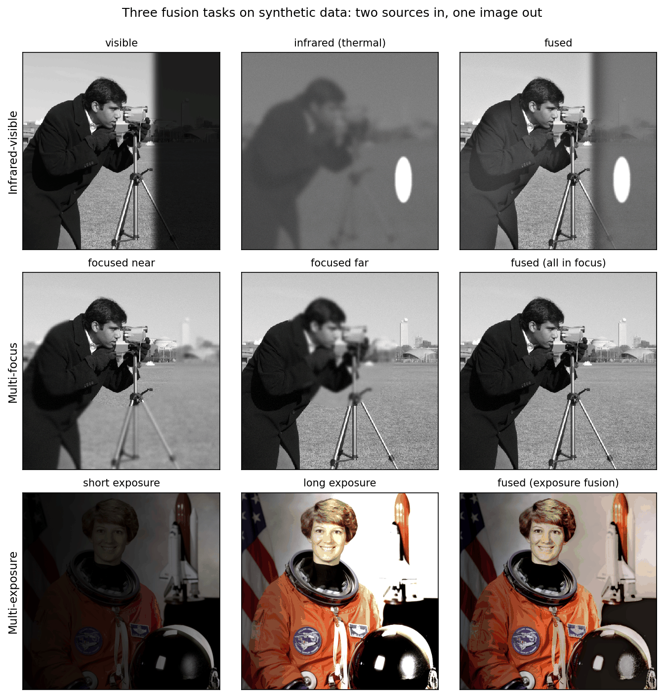
Infrared–visible fusion. A thermal camera measures infrared radiance, influenced by temperature, emissivity and reflected radiation, so a sufficiently contrasting target can stand out in darkness; visibility still depends on temperature contrast, atmosphere and sensor characteristics, while a visible camera measures reflected light and shows texture and detail in a way that matches human vision, but little in the dark [3], [2]. The goal is an image in which warm targets stand out and the background keeps its visible detail. Because the two images look so different, “keep the best of each” is ambiguous: the fused image cannot be both as bright as the thermal target and as dark as the visible shadow at the same pixel.
Multi-focus fusion. A lens has a limited depth of field: objects at one distance are sharp, nearer and farther ones are blurred. Taking several shots with different focus settings and fusing them gives an all-in-focus image (also called focus stacking or extended depth of field). An all-in-focus target is a useful ideal, and source selection approximates it where one source contains the required sharp evidence. At depth boundaries, real defocus can corrupt both sources, so neither is necessarily correct. That is why multi-focus methods often select rather than blend.
Multi-exposure fusion (MEF). A camera sensor records a limited range of brightness in one exposure. A bracket of exposures covers a wider range. The classical route is high-dynamic-range (HDR) imaging: recover the camera response and the scene radiance from the bracket [4], then compress it to a displayable image with a tone-mapping operator. Multi-exposure fusion skips the radiance step and directly blends the 8-bit exposures into a well-exposed 8-bit image [5]. It needs no camera calibration and is fast; the price is that its output is a pleasant picture, not a physical measurement.
Medical and remote-sensing fusion ask different questions
The three photographic tasks are not the whole field. The desired output can also change its number of channels and its physical interpretation.
| Scenario | Complementary evidence | Desired output | Main check |
|---|---|---|---|
| Medical multimodal fusion | CT emphasizes attenuation-related structure; MRI provides different tissue contrasts; PET/SPECT depict tracer distributions | A display combining anatomical and functional information, or features for a specified task | Anatomical alignment and preservation of modality-specific evidence |
| Pan-sharpening | A finer-resolution broad-band panchromatic image plus coarser multispectral bands | Multispectral data on a finer spatial grid | Spatial detail and spectral fidelity |
| Hyperspectral–multispectral fusion | Many narrow spectral bands at coarse resolution plus fewer broad bands at finer resolution | A finer-resolution hyperspectral cube | Agreement with both sensors’ spatial and spectral measurements |
The medical setting appears in U2Fusion’s PET–MRI evaluation [32] and DDFM’s CT/MRI and functional-imaging experiments [41]. It cannot be reduced to “copy the brighter pixel.” A bright value has a different meaning in each modality. Display fusion also does not preserve every quantitative value from both sources: retain the original data for measurements and assess any claimed diagnostic benefit through an appropriate task study.
Remote-sensing fusion often asks for an estimated multiband image rather than one pleasant grayscale display [54]. A simplified observation model makes the difference explicit:
is the unknown fine-resolution cube with narrow spectral bands. spatially blurs each band, downsamples it, and is the coarse hyperspectral observation. mixes narrow bands through spectral responses into the smaller number of multispectral bands, producing . are measurement errors. Real models also need sensor calibration, registration and potentially band-dependent blur.
For pan-sharpening, the fine-resolution observation has only one broad panchromatic band. Detail injection must account for its spectral response; its intensity is not automatically the average of the multispectral channels. At full resolution, the desired cube is usually unavailable as ground truth. Reduced-resolution experiments can create reference comparisons by degrading the available data, but conclusions depend on whether that degradation represents the real sensors.
These tasks share feature extraction and combination ideas with photographic fusion, while requiring different losses and evaluation. A model tested on infrared–visible pairs is not thereby validated for medical fusion or spectral reconstruction. “General fusion” must state whether it means a reusable architecture, separately trained models, or one checkpoint across tasks.
Registration: the step everything assumes
Plain version. Fusion compares the sources pixel by pixel, so the same pixel must show the same point in every source. If one image is shifted by a few pixels, every edge appears twice.
Registration (alignment) estimates the geometric transform between the sources and warps them onto a common grid; for moving scenes it becomes dense motion estimation, which DLCV 09A.3 explains. A static tripod reduces alignment errors, but focus changes, lens distortion and moving objects can still require registration. For infrared–visible pairs it is a real problem, and a prerequisite of fusion [3]: the two sensors differ in viewpoint, pixel distribution and resolution, so accurately registered pairs are hard to obtain, yet most existing methods need pixel-level registered pairs and existing benchmarks consist of pixel-aligned pairs [2]. We return to methods that relax this assumption at the end of the deep-learning section.
The simplest rule: averaging, and why it fades contrast
Plain version. Averaging the sources keeps a bit of everything, but anything that appears in only one source comes out at half strength. Fusion’s whole difficulty is to avoid that.
Precise version. Take two sources and that share a background , and suppose a feature of amplitude (an edge, a texture, a warm target) appears only in : , , where is the feature’s shape. The average is
so the feature’s contrast is halved. With sources and the feature in one of them, it drops to . In multi-focus fusion it is worse: the blurred source adds a blurred copy of the edge, so the average shows a sharp edge with a soft halo. In infrared–visible fusion, a target that is bright in IR and dark in the visible image ends up gray (Figure 6, last column). In multi-exposure fusion, averaging an under- and an over-exposed shot gives a flat, low-contrast image.
The fix is to make the weights depend on where each source is informative: high weight for the sharp source, the warm target, the well-exposed pixel. The rest of the classical section is about how to measure “informative” and how to change the weights without creating seams.
Multi-focus fusion: focus measures and decision maps
Plain version. Sharp regions have strong fine detail; blurred ones do not. Measure the detail around every pixel in every shot, pick the shot with the most, and copy its pixel.
Precise version. A focus measure scores how much high-frequency detail source has around pixel . A simple choice, of the kind used in classical multi-focus fusion [5], is the local energy of the Laplacian,
where is the Laplacian of the source (a second-derivative filter, see IP 03), the square makes it an energy, and denotes smoothing with a Gaussian of standard deviation , which averages the energy over a neighborhood. Blur removes high frequencies, so the in-focus source has the larger . The decision map records the winner,
where is the index of the source chosen at pixel .
A raw decision map is noisy: in flat regions (sky, a plain wall) no source has detail, and the winner is decided by noise. Two post-processing steps are standard. Cleaning removes small islands, for example with a majority vote (median filter) or morphological operations, on the assumption that in-focus regions are large and connected. Softening blurs the binary map slightly near its boundaries so that the switch from one source to another does not leave a visible seam.
The snippet builds a synthetic pair from the camera test image: inside a disk shot A is sharp, outside it shot B is sharp, and defocus is modeled as a Gaussian blur. Because we made the blur ourselves, we have the all-in-focus truth and can measure PSNR, which is impossible with real multi-focus pairs.
Code · Python · 30 lines
import numpy as np
from scipy import ndimage as ndi
from skimage import data, img_as_float
from skimage.metrics import peak_signal_noise_ratio as psnr

rng = np.random.default_rng(0)
x = img_as_float(data.camera())                       # 512 x 512: the all-in-focus "truth"
yy, xx = np.mgrid[:512, :512]
near = (yy - 200) ** 2 + (xx - 250) ** 2 < 150 ** 2   # the part that is in focus in shot A
blurred = ndi.gaussian_filter(x, 3.0)                 # defocus modeled as a Gaussian blur
A = np.where(near, x, blurred) + 0.01 * rng.standard_normal(x.shape)  # sharp inside the disk
B = np.where(near, blurred, x) + 0.01 * rng.standard_normal(x.shape)  # sharp outside it

def focus_measure(img, s=2.0):
    """Local energy of the Laplacian: large where the image has sharp detail."""
    return ndi.gaussian_filter(ndi.laplace(img) ** 2, s)

raw = focus_measure(A) > focus_measure(B)                # decision map: True = take A
clean = ndi.median_filter(raw.astype(float), 31) > 0.5   # majority vote removes small islands
w = ndi.gaussian_filter(clean.astype(float), 2.0)        # soften the seam a little

results = {"average": (A + B) / 2,
           "raw decision map": np.where(raw, A, B),
           "cleaned, soft map": w * A + (1 - w) * B}
for name, F in results.items():
    print(f"{name:18s} PSNR = {psnr(x, np.clip(F, 0, 1), data_range=1):.2f} dB")
textured = ndi.gaussian_filter(np.abs(ndi.laplace(x)), 2) > 0.01   # where the choice matters
for name, m in [("raw", raw), ("cleaned", clean)]:
    print(f"{name:7s} map agrees with the true focus map on {np.mean(m == near):.1%} of all pixels, "
          f"{np.mean((m == near)[textured]):.1%} of textured pixels")
Output
average            PSNR = 29.97 dB
raw decision map   PSNR = 39.22 dB
cleaned, soft map  PSNR = 39.81 dB
raw     map agrees with the true focus map on 80.9% of all pixels, 91.3% of textured pixels
cleaned map agrees with the true focus map on 91.2% of all pixels, 98.4% of textured pixels
The decision map wins by about 10 dB over averaging, because it copies sharp pixels instead of mixing them with blurred ones (Figure 2). Cleaning makes the map much more faithful (98.4% instead of 91.3% agreement on textured pixels), but the PSNR gain is small, 0.6 dB, because most of the raw map’s mistakes are in flat regions where shots A and B look the same anyway. These numbers are from our toy, not from any paper.
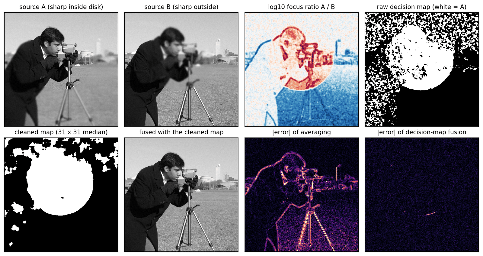
What the toy hides. Real defocus is not a Gaussian blur pasted onto a mask. Near a depth edge, the blurred foreground spreads over the background in the far-focused shot, so neither shot is sharp there. This defocus spread effect is why methods that do well on simulated data or on the popular Lytro pairs often fail on real photographs with strong defocus spread [6], [7]; Figure 6 shows it on a layered version of our toy.
Optional: The defocus spread effect (in the Supplementary notes). Why selection fails near depth edges, what a layered defocus model predicts, and what methods do about it.
Multi-scale fusion: Laplacian pyramids and wavelets
Plain version. Fuse at multiple scales: select useful fine detail and blend coarse brightness smoothly to reduce visible transitions.
The Laplacian pyramid
Precise version. The Laplacian pyramid of Burt and Adelson [8] represents an image as a stack of band-pass images plus a small low-pass residual. Let and
where blurs with a small low-pass kernel and keeps every second row and column (OpenCV’s pyrDown), upsamples by a factor of 2 and interpolates with the same kernel (pyrUp), is the Gaussian pyramid level (a blurred, smaller copy of the image) and the Laplacian pyramid level , the detail that has and the coarser level does not. The top of the pyramid is the residual . Level has times the width and height of the image. The image is recovered exactly by the collapse
and . Exactness holds for any , because each stores exactly what fails to predict. The name comes from the authors’ observation that the encoding is equivalent to sampling the image with Laplacian operators of many scales [8].
Optional: Building and collapsing a Laplacian pyramid (in the Supplementary notes). The kernel, the size bookkeeping for odd image sizes, why reconstruction is exact, and how many levels to use.
Fusing two pyramids
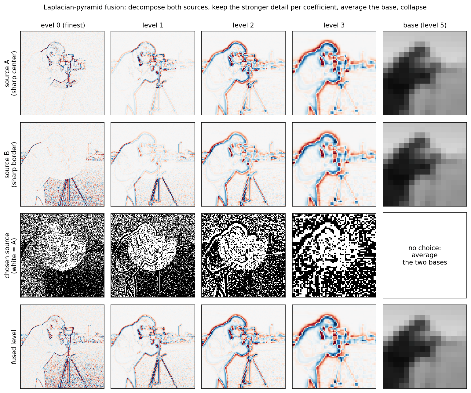
Pyramid fusion decomposes each source, combines the pyramids level by level, and collapses the result. Classic pyramid fusion selects the most salient Laplacian coefficients of the sources [9], [5]; a simple version of the rule has two parts:
where , and are level of the pyramids of source A, source B and the fused image. The max-abs rule keeps, at every position and scale, the coefficient with the larger magnitude, which is the stronger local feature; the coarse residual is averaged because it carries overall brightness, where no source should simply win. Selecting per coefficient at every scale means the switch between sources is spread over the support of the pyramid’s filters, which is wider at coarser levels; this is the multiresolution blending idea that Burt and Adelson introduced for joining image mosaics without visible seams [10]. Burt and Kolczynski later refined pyramid fusion to make it more robust to small shifts and noise and to handle features of similar salience but opposite contrast [9].
The snippet continues from the multi-focus example (it uses A, B, x and psnr).
Code · Python · 35 lines
import cv2
import pywt

def laplacian_pyramid(img, levels=5):
    G = [img.astype(np.float32)]
    for _ in range(levels):
        G.append(cv2.pyrDown(G[-1]))                      # blur, then keep every 2nd pixel
    L = [G[i] - cv2.pyrUp(G[i + 1], dstsize=G[i].shape[::-1]) for i in range(levels)]
    return L + [G[-1]]                                    # band-pass details + coarse base

def collapse(L):
    img = L[-1]
    for detail in reversed(L[:-1]):
        img = cv2.pyrUp(img, dstsize=detail.shape[::-1]) + detail
    return img

def pick_stronger(p, q):
    return np.where(np.abs(p) >= np.abs(q), p, q)         # "max-abs" selection rule

def pyramid_fuse(a, b, levels=5):
    La, Lb = laplacian_pyramid(a, levels), laplacian_pyramid(b, levels)
    fused = [pick_stronger(p, q) for p, q in zip(La[:-1], Lb[:-1])]
    fused.append((La[-1] + Lb[-1]) / 2)                   # base: average the coarse level
    return collapse(fused).astype(float)

def wavelet_fuse(a, b, wavelet="db2", levels=4):
    ca, cb = pywt.wavedec2(a, wavelet, level=levels), pywt.wavedec2(b, wavelet, level=levels)
    fused = [(ca[0] + cb[0]) / 2]                         # approximation band: average
    for da, db in zip(ca[1:], cb[1:]):                    # (H, V, D) detail bands per level
        fused.append(tuple(pick_stronger(p, q) for p, q in zip(da, db)))
    return pywt.waverec2(fused, wavelet)

print(f"pyramid reconstruction error: {np.abs(collapse(laplacian_pyramid(A)) - A).max():.1e}")
for name, F in [("Laplacian pyramid", pyramid_fuse(A, B)), ("wavelet (db2)", wavelet_fuse(A, B))]:
    print(f"{name:18s} PSNR = {psnr(x, np.clip(F, 0, 1), data_range=1):.2f} dB")
Output
pyramid reconstruction error: 5.9e-08
Laplacian pyramid  PSNR = 37.60 dB
wavelet (db2)      PSNR = 36.43 dB
The reconstruction error of about is single-precision rounding: the pyramid itself is lossless. Pyramid fusion beats averaging by more than 7 dB but stays about 2 dB below the decision map. The reason is visible in Figure 3: the per-coefficient choice is noisy, especially at fine levels, where the blurred source’s noise sometimes wins in flat areas. Comparing smoothed coefficient energies instead of single coefficients, the “area-based” selection of Li et al. [11], closes most of the gap (Exercise 3). The general lesson: when the true answer is a selection (multi-focus), spatially coherent decisions beat per-coefficient ones.
Wavelet fusion
Wavelet fusion follows the same plan with the discrete wavelet transform of IP 07 instead of the pyramid: decompose both sources, keep the stronger detail coefficient in each horizontal, vertical and diagonal band, average the approximation band, and invert. Li, Manjunath and Mitra [11] proposed it with an area-based maximum-selection rule (compare activity over a small window, not single coefficients) and a consistency verification step that makes a coefficient follow the choice of its neighbors, and argued that the wavelet transform’s compactness, orthogonality and directional selectivity make it better suited than the Laplacian pyramid. In our toy, the simple per-coefficient rule gives 36.43 dB, about 1 dB below the pyramid. One known weakness is that the decimated wavelet transform is not shift-invariant: shifting the image by one pixel changes its coefficients, so a per-coefficient decision can change too. Greater shift invariance was also one of the aims of Burt and Kolczynski’s refinement of pyramid fusion [9].
Exposure fusion: well-exposed images without HDR
Plain version. Exposure fusion weights contrast, saturation and well-exposedness, then blends through image pyramids to reduce seams.
Precise version. Mertens, Kautz and Van Reeth [5] compute, for exposure at pixel , three quality measures:
- contrast : the absolute response of a Laplacian filter applied to the grayscale exposure (high at edges and texture);
- saturation : the standard deviation of the R, G and B values at the pixel (vivid colors have a large spread, washed-out ones a small spread);
- well-exposedness : a Gaussian bump around mid-gray, applied to each color channel and multiplied, with in their implementation.
They are combined by a product with exponents and normalized over the exposures:
where set the influence of each measure (an exponent of 0 switches a measure off) and is the normalized weight, which sums to 1 over the exposures at each pixel. The product acts like an “and”: a pixel gets a high weight only if it is detailed and colorful and well exposed [5].
Why a pyramid. Blending pixels directly, , produces visible seams wherever the weights change quickly, because the exposures have very different absolute brightness [5]. Smoothing the weights with a Gaussian removes the seams but creates halos around edges. Exposure fusion instead blends per pyramid level: each Laplacian level of each exposure is weighted by the matching level of a Gaussian pyramid of its weight map,
where is level of a Laplacian pyramid and level of a Gaussian pyramid; the result is obtained by collapsing [5]. Fine detail is blended with sharp weights and coarse brightness with very smooth weights, which reduces seams and halos when alignment and pyramid settings are appropriate.
The snippet builds a synthetic scene with an 8-stop light falloff (dark on the left, bright on the right), photographs it with three exposure times through a simple camera model (gamma, clipping, 8-bit quantization), and fuses the bracket. It checks the result against OpenCV’s implementation, cv2.createMergeMertens.
Code · Python · 56 lines
import numpy as np
import cv2
from skimage import data, img_as_float

# A synthetic high-dynamic-range scene: linear radiance times a light falloff of 8 stops.
rgb = img_as_float(data.astronaut()) ** 2.2                       # undo display gamma -> linear
light = 2.0 ** np.linspace(-6, 2, rgb.shape[1])[None, :, None]    # dark left, bright right
radiance = rgb * light

def camera(E, t):
    """Expose for time t, apply a 1/2.2 display gamma, clip and quantize to 8 bits."""
    return np.round(np.clip((t * E) ** (1 / 2.2), 0, 1) * 255) / 255

stack = [camera(radiance, t) for t in (1 / 8, 1.0, 8.0)]          # under, middle, over

def mertens_weights(imgs, sigma=0.2, eps=1e-12):
    W = []
    for I in imgs:
        gray = I.mean(axis=2).astype(np.float32)
        C = np.abs(cv2.Laplacian(gray, cv2.CV_32F))                # contrast
        S = I.std(axis=2)                                         # saturation
        E = np.prod(np.exp(-(I - 0.5) ** 2 / (2 * sigma ** 2)), axis=2)  # well-exposedness
        W.append(C * S * E + eps)
    W = np.array(W)
    return W / W.sum(axis=0)                                      # weights sum to 1 per pixel

def gauss_pyr(img, n):
    G = [img.astype(np.float32)]
    for _ in range(n):
        G.append(cv2.pyrDown(G[-1]))
    return G

def lap_pyr(img, n):
    G = gauss_pyr(img, n)
    return [G[i] - cv2.pyrUp(G[i + 1], dstsize=G[i].shape[1::-1]) for i in range(n)] + [G[-1]]

def exposure_fusion(imgs):
    n = int(np.log2(min(imgs[0].shape[:2])))                      # full depth: 9 levels for 512 px
    fused = None
    for I, Wk in zip(imgs, mertens_weights(imgs)):
        level = [g[..., None] * l for g, l in zip(gauss_pyr(Wk, n), lap_pyr(I, n))]
        fused = level if fused is None else [f + l for f, l in zip(fused, level)]
    out = fused[-1]
    for detail in reversed(fused[:-1]):
        out = cv2.pyrUp(out, dstsize=detail.shape[1::-1]) + detail
    return np.clip(out, 0, 1)

R = exposure_fusion(stack)
naive = np.clip(np.sum(mertens_weights(stack)[..., None] * np.array(stack), axis=0), 0, 1)
ref = cv2.createMergeMertens(1.0, 1.0, 1.0).process(
    [(255 * I[..., ::-1]).round().astype(np.uint8) for I in stack])[..., ::-1]   # OpenCV uses BGR
for name, I in [("under", stack[0]), ("middle", stack[1]), ("over", stack[2]),
                ("per-pixel blend", naive), ("pyramid blend", R)]:
    ok = np.mean(np.all((I > 0.05) & (I < 0.95), axis=2))        # no channel near black or clipped
    print(f"{name:15s} well-exposed pixels: {100 * ok:4.1f}%")
print(f"mean |ours - OpenCV MergeMertens| = {np.abs(R - np.clip(ref, 0, 1)).mean():.4f}")
Output
under           well-exposed pixels: 45.8%
middle          well-exposed pixels: 58.7%
over            well-exposed pixels: 41.2%
per-pixel blend well-exposed pixels: 72.3%
pyramid blend   well-exposed pixels: 73.8%
mean |ours - OpenCV MergeMertens| = 0.0027
Our implementation agrees with OpenCV’s to within 0.003 on a scale; the small difference presumably comes from implementation details such as pyramid depth, border handling and input rounding. The crude “well-exposed pixels” count rises from at most 59% for any single exposure to 74% after fusion. Note what the count misses: the per-pixel blend scores almost as well (72%) yet looks badly broken, with seams and speckle where the weights jump (Figure 4, bottom left). A single number does not see artifacts, a theme the evaluation section returns to.
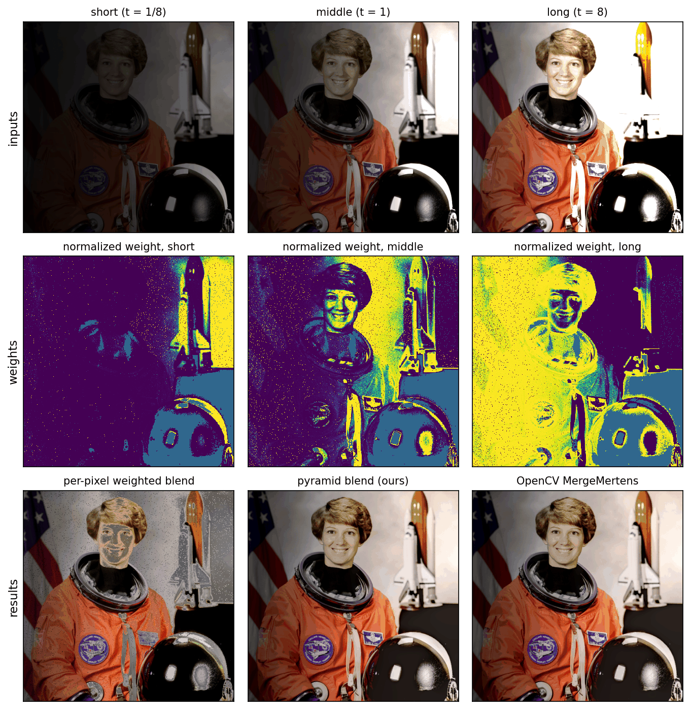
Exposure fusion is not HDR. The output keeps no radiance values, so it cannot be relit or re-exposed, and with strongly varying brightness the multiresolution blend can create a spurious low-frequency brightness change; Mertens et al. note that a taller pyramid partly solves it [5]. Exposure fusion also assumes perfectly aligned exposures, possibly after registration [5]; with camera or object motion, the result shows ghosts (Figure 6). Finally, Mertens et al. compare their blending with earlier pyramid fusion that selects the most salient coefficients and find the selection results too dark and with color shifts on exposure stacks [5]: for exposures, blending beats selecting, the opposite of multi-focus fusion.
Optional: Exposure fusion (Mertens, Kautz and Van Reeth) (in the Paper guides). What the paper set out to do, what its comparison figures show, and the limitations it states.
Two more classical tools: guided filtering and sparse codes
Plain version. Two later ideas improved the classical rules: make the weight maps follow object edges using an edge-aware filter, and describe image patches with a learned dictionary so that “how much detail” is measured on a richer representation.
Guided-filtering fusion (GFF). Li, Kang and Hu [12] split each source into a base layer (large-scale intensity variations) and a detail layer (small-scale detail), and fuse each layer with a weighted average whose weight maps are refined by the guided filter [13] so that they respect spatial consistency, that is, neighboring pixels with similar intensities get similar weights. The guided filter is explained in IP 03, and its learned and fast variants in DLCV 09C. The authors report state-of-the-art results at the time for multispectral, multi-focus, multimodal and multi-exposure images with one method [12]. The design shows the general recipe of the classical era: a two- or multi-scale decomposition, an activity measure, and a smoothing step that turns the activity into clean weights.
Sparse-representation (SR) fusion. Yang and Li [14] represent the sources with sparse coefficients over an overcomplete dictionary, combine the coefficients with a choose-max rule, and reconstruct the fused image from the combined coefficients and the dictionary; by changing the approximation criterion of the sparse coding, the same scheme also restores noisy sources while fusing them. Later work learned the dictionary from the source patches themselves [15]. SR methods were among the strongest classical multi-focus methods, but they are slow: in one benchmark they took more than seven minutes to fuse an image pair [7].
Optional: Sparse-representation fusion (in the Supplementary notes). The sparse coding model, the patch-by-patch fusion steps, the activity measure and where the cost comes from.
Evaluating fusion without ground truth
Plain version. Without a correct fused image to compare with, fusion is scored by rules of thumb: does the result have a lot of detail, a lot of contrast, a lot of information from the sources? Each rule captures one aspect, so they disagree, and a method can be tuned to look good on the chosen ones.
This section comes before deep learning on purpose: deep fusion networks are trained with losses built from the same ingredients as these metrics, so understanding the metrics explains the losses.
Why fusion has no single right answer
For multi-focus fusion on synthetic data, the all-in-focus image is known and PSNR or SSIM [16] against it is meaningful, as in our first snippet. For infrared–visible and multi-exposure fusion, no such image exists, and benchmark studies agree that no single metric is better than all others [17], [18], [7]. Benchmarks therefore report many metrics: VIFB implements 13 [17], and the multi-exposure benchmark MEFB and the multi-focus benchmark MFIFB 20 each [18], [7]. VIFB groups them into four families: information-theory-based, image-feature-based, structural-similarity-based and human-perception-based [17]. Its results show the consequence: one method wins the information-theory metrics, another the feature-based ones and a third the structural ones, and no method wins all [17].
Optional: VIFB: a visible and infrared image fusion benchmark (in the Paper guides). How the benchmark was built, how to read its tables, and why its best-scoring methods looked worst.
Metrics that look only at the fused image
Let be the fused image, of size , with values in .
Entropy (EN) measures how spread out the histogram is:
where is the number of gray levels (histogram bins) and the fraction of pixels in bin . EN is in bits; a larger value means the gray levels are used more evenly. It is easily affected by noise, so benchmark studies use it only as an auxiliary metric [18].
Standard deviation (SD) measures global contrast, , where is the mean of (some implementations omit the , which changes the scale; rankings are unchanged only when the compared images have the same dimensions).
Spatial frequency (SF) measures the overall activity of neighboring differences [19], [18]:
where RF (row frequency) uses horizontal differences and CF (column frequency) vertical ones; normalizations differ between implementations. Large SF means many strong edges and much texture.
These three never look at the sources. They reward “more”: more gray levels, more contrast, more edges. Noise supplies all three for free.
Metrics that compare with the sources
Mutual information (MI) measures how much the fused image tells about each source [20]:
where is the joint histogram of source and (normalized to sum to 1), and , its marginals. MI is large when the gray level of predicts the gray level of each source well (see IT 01 for the definition). Hossny, Nahavandi and Creighton showed analytically that this classic MI sum is not a valid fusion performance measure on its own [21], and benchmark toolkits implement a normalized version attributed to them, which divides each term by the sum of the two entropies [18].
Optional: Mutual information as a fusion metric (in the Supplementary notes). Why copying one source scores well, how the bin count changes the value, and what normalization fixes.
Gradient-based fusion performance (Xydeas and Petrović [22]) measures how much edge information of the sources survives in . At every pixel it compares the edge strength and orientation (from image gradients) of each source with those of , turns the comparison into a preservation value , the product of an edge-strength and an orientation preservation value, and averages with weights that express the importance of each source [18]:
A value near 1 means the edges of both sources are kept with their strength and direction. The snippet below implements a simplified version, which we call : the strength preservation is the ratio of the smaller to the larger gradient magnitude, the orientation preservation falls linearly with the angle between the edges, and the weights are the source gradient magnitudes. Use a reference implementation when you report .
Structure-based and perception-based metrics. Piella and Heijmans [23] proposed three variants of a fusion quality metric based on an image quality index of Wang and Bovik; they need no ground-truth image because they compare with the sources, and the authors found them consistent with subjective evaluations. VIFF [24] adapts the visual information fidelity criterion to fusion and computes it over several resolutions. For multi-exposure fusion, MEF-SSIM [25] was designed from a subjective study: its authors found that general fusion metrics predicted the perceived quality of multi-exposure fusion poorly, and built an SSIM-style index around a patch structure consistency measure that correlates much better with human judgments. Liu et al. [26] compared twelve fusion metrics over six multiresolution fusion algorithms for night-vision applications.
VIF is an information-transfer model, not raw entropy. It estimates how much modeled source information survives through the candidate image and a visual channel [55]. Fusion variants aggregate source comparisons differently, so values above one or different paper scales require checking the implementation. A source still is not a true fused target.
Optional: VIF and source-referenced fusion scores (in the Supplementary notes). The information ratio, its channel assumptions and why fusion aggregation changes the score.
A toy that fools the metrics
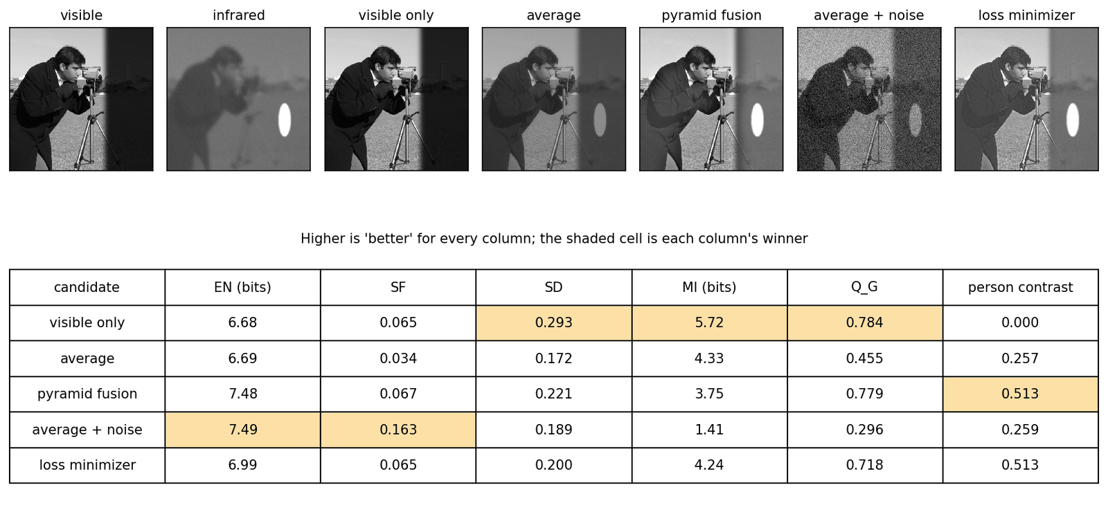
The snippet builds an infrared–visible pair from the camera image: the visible image has a deep shadow on the right in which a person is invisible; the thermal image is smooth, with little texture, and the person glows. It scores four candidates: no fusion at all (the visible image), the average, pyramid fusion (max-abs details, and the brighter of the two coarse bases so that the warm target keeps its level), and the average with added noise. As an independent check of what a user cares about, it also measures the person contrast: the mean of on the person minus the mean on a ring around them.
Code · Python · 76 lines
import numpy as np
import cv2
from scipy import ndimage as ndi
from skimage import data, img_as_float

rng = np.random.default_rng(1)
scene = img_as_float(data.camera())
yy, xx = np.mgrid[:512, :512]
person = ((yy - 330) / 60) ** 2 + ((xx - 420) / 22) ** 2 < 1        # a warm "person", 120 px tall
shadow = ndi.gaussian_filter((xx > 340).astype(float), 8)          # a dark area on the right
vis = scene * (1 - 0.85 * shadow)                                  # visible: person hidden in shadow
ir = 0.25 + 0.3 * ndi.gaussian_filter(scene, 6)                    # thermal: smooth, little texture
ir = np.clip(ir + 0.6 * ndi.gaussian_filter(person.astype(float), 2)  # the warm body glows
             + 0.01 * rng.standard_normal(ir.shape), 0, 1)

def lap_pyr(img, n=5):
    G = [img.astype(np.float32)]
    for _ in range(n):
        G.append(cv2.pyrDown(G[-1]))
    return [G[i] - cv2.pyrUp(G[i + 1], dstsize=G[i].shape[::-1]) for i in range(n)] + [G[-1]]

def collapse(L):
    img = L[-1]
    for d in reversed(L[:-1]):
        img = cv2.pyrUp(img, dstsize=d.shape[::-1]) + d
    return img

def pyramid_fuse(a, b):                    # max-abs details, and the brighter coarse base
    La, Lb = lap_pyr(a), lap_pyr(b)
    out = [np.where(np.abs(p) >= np.abs(q), p, q) for p, q in zip(La[:-1], Lb[:-1])]
    out.append(np.maximum(La[-1], Lb[-1]))
    return np.clip(collapse(out), 0, 1).astype(float)

def entropy(F, bins=256):
    p = np.histogram(F, bins, (0, 1))[0] / F.size
    p = p[p > 0]
    return -np.sum(p * np.log2(p))

def spatial_frequency(F):
    rf = np.mean(np.diff(F, axis=1) ** 2)            # row frequency: horizontal differences
    cf = np.mean(np.diff(F, axis=0) ** 2)            # column frequency: vertical differences
    return np.sqrt(rf + cf)

def mutual_info(X, F, bins=64):
    pxy = np.histogram2d(X.ravel(), F.ravel(), bins, [[0, 1], [0, 1]])[0] / X.size
    px, pf = pxy.sum(1, keepdims=True), pxy.sum(0, keepdims=True)
    nz = pxy > 0
    return np.sum(pxy[nz] * np.log2(pxy[nz] / (px @ pf)[nz]))

def q_gradient(A, B, F):
    """A simplified Q^{AB/F}: how well F keeps the edge strength and direction of A and B."""
    def grad(I):
        gx, gy = ndi.sobel(I, 1), ndi.sobel(I, 0)
        return np.hypot(gx, gy), np.arctan2(gy, gx)
    gF, aF = grad(F)
    num = den = 0.0
    for X in (A, B):
        gX, aX = grad(X)
        strength = np.minimum(gX, gF) / (np.maximum(gX, gF) + 1e-12)
        d = np.abs(aX - aF) % np.pi                  # edge direction is defined modulo pi
        direction = 1 - np.minimum(d, np.pi - d) / (np.pi / 2)
        num += np.sum(strength * direction * gX)     # weight each pixel by the source edge strength
        den += np.sum(gX)
    return num / den

ring = ndi.binary_dilation(person, iterations=15) & ~person
candidates = {"visible only": vis,
              "average": (vis + ir) / 2,
              "pyramid fusion": pyramid_fuse(vis, ir),
              "average + noise": np.clip((vis + ir) / 2 + 0.08 * rng.standard_normal(vis.shape), 0, 1)}
print(f"{'':16s}  EN    SF     SD     MI    Q_G   person contrast")
for name, F in candidates.items():
    mi = mutual_info(vis, F) + mutual_info(ir, F)
    tc = F[person].mean() - F[ring].mean()           # task check: does the person stand out?
    print(f"{name:16s} {entropy(F):4.2f}  {spatial_frequency(F):.3f}  {F.std():.3f}  {mi:4.2f}  "
          f"{q_gradient(vis, ir, F):.3f}  {tc:6.3f}")
Output
                  EN    SF     SD     MI    Q_G   person contrast
visible only     6.68  0.065  0.293  5.72  0.784  -0.000
average          6.69  0.034  0.172  4.33  0.455   0.257
pyramid fusion   7.48  0.067  0.221  3.75  0.779   0.513
average + noise  7.49  0.163  0.189  1.41  0.296   0.259
Read the table column by column (all numbers are from this toy):
- Noise wins EN and SF. Adding noise to the average gives the highest entropy and almost five times the average’s spatial frequency, while making the image worse.
- Not fusing at all wins SD, MI and . The visible image alone has the most contrast, the highest mutual information (copying a source makes equal to that source’s entropy) and even the highest edge score, because the strong visible edges carry most of the weight . Yet the person is invisible: its contrast is zero (printed as -0.000).
- Pyramid fusion wins only the task check. It doubles the person’s contrast relative to the average while keeping the visible texture ( almost as high as the visible image), but it is not the best on any of the five standard metrics.
What to report
The toy is extreme on purpose, but each effect appears in practice: noise and over-sharpening raise EN, SF and SD; results that look like one source score well on MI; and metrics with source-dependent weights favor the source with stronger edges. Benchmark authors draw the same conclusion from real methods: researchers tend to pick the metrics that support their method [17], [7], and quantitative and qualitative comparisons may disagree [7]. Practical advice:
- Report several metrics from different families, including at least one that compares with the sources (, an SSIM-based score or VIFF), never only EN, SD or SF.
- Use reference-based metrics where a reference can exist: synthetic multi-focus pairs, or multi-exposure datasets with selected references (with the caveat that the reference is one acceptable answer).
- Add a downstream task when fusion feeds one, such as detection or segmentation accuracy on the fused images, as recent infrared–visible benchmarks do [27], [28].
- Show crops of hard regions (depth edges, highlights, warm targets in shadow), and run a user study when the claim is about visual quality.
Deep image fusion
Plain version. Deep networks learn the weights, the features and the combination rule from data. The catch is that there are no examples of the correct output, so the network is trained to satisfy rules of the same kind as the metrics above.
The missing ground truth
A restoration network (DLCV 09) learns from pairs (degraded input, clean target). A fusion network has inputs but no target. The field uses four ways around this:
- Synthesize a task that has ground truth. For multi-focus fusion, blur parts of sharp images: the sharp image is the target and the blur mask the true decision map. Most deep multi-focus methods are trained this way [7]; IFCNN trains a general fusion network on a synthetic multi-focus dataset built from an RGB-D dataset, so that ground-truth fused images exist [29].
- Train something else, then fuse features by a rule. Train an autoencoder to reconstruct ordinary images, then at test time encode both sources, merge the features with a hand-made rule and decode [30].
- Unsupervised losses. Define a loss that measures how well keeps the intensity, gradients or structure of each source, and train the network to minimize it on unlabeled source pairs [31], [32].
- Let another task supervise. Feed to a detector or segmenter and add its loss, so that the fusion is judged by its usefulness [33], [27].
Unsupervised losses
A recent survey groups the losses of unsupervised infrared–visible fusion into pixel-level terms (L1 or MSE), terms built from evaluation metrics (above all SSIM) and terms that target data characteristics such as image gradients [2]. A typical combination is
where is an intensity target built from the sources (for example a weighted average, or the pixel-wise maximum, which keeps the brighter thermal target), a gradient-magnitude target (for example the larger of the two sources’ gradient magnitudes at each pixel), the structural similarity [16] between and source , per-source weights, and the s weight the terms. Methods differ mainly in these choices: DeepFuse [31] trains with MEF-SSIM [25] alone, SwinFusion [34] with SSIM, texture and intensity terms, and U2Fusion [32] weights a similarity loss by an estimate of how much information each source holds.
Optional: Training signals of representative fusion networks (in the Supplementary notes). What DenseFuse, DeepFuse, U2Fusion, SwinFusion, FusionGAN, CDDFuse, DDFM and EMMA actually optimize, and what each choice implies for the result.
The loss defines the answer
Plain version. If nobody gives the network a target, the loss is the target. The best a network can do is to output, for each pair, the image that minimizes the loss. For a simple quadratic loss we can compute that image directly, without any network, and look at it.
The snippet continues from the toy of the evaluation section (it uses vis, ir, person, ring and the metric functions). It minimizes a squared-error version of the loss above, an intensity term toward the pixel-wise maximum of the sources plus a gradient term toward the stronger source gradient,
where stacks the horizontal and vertical forward differences of , takes, at each position and in each direction, the difference of whichever source has the larger one in magnitude, and trades intensity against gradients. Setting the gradient of the objective to zero gives a sparse linear system, , where is the difference operator; conjugate gradients solves it in seconds.
Code · Python · 29 lines
import scipy.sparse as sp
from scipy.sparse.linalg import cg

def diff_ops(H, W):
    d = lambda n: sp.diags([-np.ones(n - 1), np.ones(n - 1)], [0, 1], shape=(n - 1, n))
    return sp.kron(sp.eye(H), d(W)).tocsr(), sp.kron(d(H), sp.eye(W)).tocsr()  # Dx, Dy

def fuse_by_loss(a, b, lam=10.0):
    """Minimize ||F - max(a, b)||^2 + lam * ||grad F - g||^2, where g is the stronger source gradient."""
    H, W = a.shape
    Dx, Dy = diff_ops(H, W)
    gx = [Dx @ s.ravel() for s in (a, b)]
    gy = [Dy @ s.ravel() for s in (a, b)]
    pick_x = np.abs(gx[0]) >= np.abs(gx[1])
    pick_y = np.abs(gy[0]) >= np.abs(gy[1])
    tx, ty = np.where(pick_x, gx[0], gx[1]), np.where(pick_y, gy[0], gy[1])
    target = np.maximum(a, b).ravel()                 # intensity term: the brighter source
    M = sp.eye(H * W) + lam * (Dx.T @ Dx + Dy.T @ Dy)  # normal equations of the quadratic loss
    rhs = target + lam * (Dx.T @ tx + Dy.T @ ty)
    f, info = cg(M, rhs, x0=target, rtol=1e-6, maxiter=2000)
    if info != 0: raise RuntimeError("Conjugate gradient did not converge")
    return np.clip(f.reshape(H, W), 0, 1)

for lam in (1.0, 10.0):
    F = fuse_by_loss(vis, ir, lam)
    mi = mutual_info(vis, F) + mutual_info(ir, F)
    print(f"loss minimizer, lam={lam:4.1f}: EN {entropy(F):.2f}  SF {spatial_frequency(F):.3f}  "
          f"SD {F.std():.3f}  MI {mi:.2f}  Q_G {q_gradient(vis, ir, F):.3f}  "
          f"person contrast {F[person].mean() - F[ring].mean():.3f}")
Output
loss minimizer, lam= 1.0: EN 6.91  SF 0.060  SD 0.195  MI 4.68  Q_G 0.659  person contrast 0.513
loss minimizer, lam=10.0: EN 6.99  SF 0.065  SD 0.200  MI 4.24  Q_G 0.718  person contrast 0.513
The loss minimizer has the person as bright as pyramid fusion does (contrast 0.513) and keeps the visible texture (Figure 5, right). Raising from 1 to 10 raises and SF and lowers MI: the weight between loss terms moves the result along the metrics, and choosing it is choosing what the “correct” fusion is. This is the honest summary of unsupervised deep fusion. The network adds speed, the ability to generalize from many training pairs and features richer than raw gradients, but the definition of a good result is still written by hand, in the loss.
Families of deep fusion networks
The surveys organize the field by architecture and by training strategy [35], [2]. The table lists representative members of each family; the infrared–visible survey guide in the Paper guides covers the taxonomy in more depth.
| Family | Idea | Representative methods |
|---|---|---|
| Learned decision maps or weights | A network predicts which source is in focus, or a per-pixel weight; the output is still a selection or blend of source pixels | CNN focus map for multi-focus [36]; MEF-Net predicts weights at low resolution and upsamples them with a guided filter [37] |
| Autoencoder + fusion rule | Train an encoder–decoder to reconstruct images; fuse encoded features with a hand-made rule | DenseFuse [30] |
| End-to-end, unsupervised | A network maps the sources to , trained with an intensity/gradient/SSIM-type loss | DeepFuse [31], U2Fusion [32], SwinFusion [34], CDDFuse [38] |
| Supervised on synthetic data | Train on synthesized pairs with a known fused image | IFCNN [29] |
| Adversarial (GAN) | A discriminator pushes to look like one source’s texture while a content loss keeps the other’s intensity | FusionGAN [39], TarDAL [27] |
| Task-driven | A detection or segmentation loss on guides the fusion network | SeAFusion [33], TarDAL [27], SegMiF [28], TDFusion [40] |
| Generative priors and language | A pretrained diffusion model or a text encoder guides the fusion | DDFM [41], Text-IF [42] |
Two families rely on generative models explained elsewhere: GANs in ML 07 and diffusion models in ML 08. Across all families, the architecture matters less for the character of the result than the training signal, which is what the table’s middle column really distinguishes.
What each learned family actually learns
The architecture table is a map, not a training recipe. Follow the source of supervision to understand the result.
Autoencoder plus a rule. DenseFuse learns features and reconstruction from ordinary images [30]. At inference, a fixed rule merges source features. It needs no fused target for training, but reconstruction alone does not teach which modality should win. Addition and activity weighting encode different preferences even with identical network weights.
Supervised convolutional fusion. IFCNN learns from synthetic pairs with a known target and merges source features through an element-wise operation [29]. This supplies direct supervision but transfers the synthetic data’s assumptions into the model. A blur process that ignores foreground spread or sensor differences may teach the wrong decision on real pairs.
Direct unsupervised fusion. U2Fusion trains the generated image to resemble sources under adaptive information weights [32]. Both its structural and intensity terms are needed to understand the output. Its VGG-based weights and continual-learning penalty operate during training; the final image generator does not need VGG or EWC at inference.
Adversarial fusion. FusionGAN adds a discriminator to a source-preservation objective, encouraging visible-like texture while retaining infrared intensity [39]. A realistic appearance is a distributional preference, not proof that a particular edge is supported by the sources. TarDAL splits the adversarial roles between thermal targets and visible details and adds downstream supervision [27].
Attention-based fusion. SwinFusion learns within-source and cross-source interactions with windowed and shifted-window attention [34]. Queries, keys and values let one feature use evidence from another location or modality. Windowing controls cost; successive shifted windows extend interaction across boundaries. Attention still needs a fusion objective and aligned evidence, and it can transfer noise as well as useful texture.
Diffusion-based fusion. DDFM repeatedly combines a pretrained denoising prior with source-informed corrections [41]. It avoids fusion-specific denoiser training but pays for iterative inference. One EM correction inside a diffusion step is not one-step fusion. The modeled likelihood and image prior both influence what the sampler produces.
Unified and task-aware systems. “Unified” may mean one loss design or one architecture rather than one set of weights; check the checkpoint and training setting. U2Fusion explicitly targets shared parameters across tasks [32]. Task-aware models instead judge fusion partly through a detector or segmenter [27], [33]. They need the corresponding supervision and can specialize to that task. Neither label guarantees that a single model handles arbitrary modalities or unregistered inputs.
Optional: DenseFuse, U2Fusion, TarDAL and DDFM (in the Paper guides). The full design, experiment settings, ablations and limitations of each approach.
Fusion for downstream tasks
Plain version. If the fused image feeds a detector, the best fusion is the one that makes the detector work, not the one with the best entropy.
SeAFusion [33] cascades a real-time fusion network with a segmentation network and adds a semantic loss, training the two in a loop [2]. TarDAL [27] writes fusion and detection as one bilevel optimization problem, unrolls it into a fusion network with one generator and two discriminators (one for the infrared targets, one for visible texture) followed by a detector, and introduces the M3FD benchmark captured with a synchronized infrared–visible system. SegMiF [28] exchanges intermediate features between a fusion and a segmentation sub-network through hierarchical attention, and collects a full-time benchmark with 15 annotated pixel-level classes. TDFusion [40] goes one step further and learns the fusion loss itself: a loss-generation module is trained by meta-learning so that the fusion network it supervises minimizes the downstream task loss. Task-driven training answers the “what is correct?” question with a measurable goal, but it optimizes for one task and one network, and task performance does not fully reflect visual quality [2].
Fusing images that are not aligned
Plain version. Real infrared and visible cameras are rarely perfectly aligned. Registration-robust methods estimate the misalignment and correct it inside the fusion network.
Pixel-wise fusion of misaligned pairs produces ghosts and double edges around objects [43], [44]. Two strategies appear in recent work [2]. The style-transfer route first translates one modality into the other, so that cross-modal registration becomes a single-modality one: UMF-CMGR [43] generates a pseudo-infrared image from the visible image, registers the real infrared image to it with a multi-level registration network, and then fuses. The shared-feature route maps both modalities into a common feature space and predicts deformation fields there. SuperFusion [44] combines registration (bidirectional deformation fields), fusion and a semantic constraint from a pretrained segmentation model in one framework. Multi-exposure fusion has the analogous problem with camera shake and moving objects (ghosting).
Datasets and benchmarks
Plain version. Infrared–visible fusion has several public collections of aligned pairs, some with object labels; multi-focus and multi-exposure fusion have smaller test sets and benchmark toolkits. None has a ground-truth fused image for real infrared–visible data.
| Dataset | Task | Content (as described by its authors) |
|---|---|---|
| TNO [45] | IR–visible | Intensified visual, near-infrared and long-wave infrared night-time images of military and surveillance scenes |
| RoadScene [32] | IR–visible | 221 aligned pairs of road scenes selected from FLIR videos, released with U2Fusion |
| MSRS [46] | IR–visible | 1,444 aligned pairs of road scenes, built from the MFNet dataset [47] by removing 125 misaligned pairs and enhancing the infrared images |
| LLVIP [48] | IR–visible | 15,488 strictly aligned pairs, mostly taken in very dark scenes, with pedestrian labels |
| M3FD [27] | IR–visible | 4,200 registered pairs with detection labels, plus 300 pairs from independent scenes for fusion; images mostly 1024 × 768 |
| FMB [28] | IR–visible | A full-time benchmark with 15 annotated pixel-level classes for fusion and segmentation |
| VIFB [17] | IR–visible | A test set of 21 pairs, a code library of 20 fusion algorithms and 13 metrics |
| Lytro [15] | Multi-focus | 20 pairs of multi-focus images, long the most widely used test set [7] |
| MFFW [6] | Multi-focus | 19 real pairs collected from the Internet with a strong defocus spread effect |
| MFIFB [7] | Multi-focus | A benchmark of 105 test pairs, 30 algorithms and 20 metrics |
| SICE [49] | Multi-exposure | 589 multi-exposure sequences (4,413 images), each with a reference chosen by subjective comparison of 13 fusion and HDR algorithms |
| MEFB [18] | Multi-exposure | A benchmark of 100 test image pairs, 16 algorithms and 20 metrics |
Read the table with three cautions. Preprocessing is part of the data: RoadScene’s infrared images had their background thermal noise processed, and MSRS’s infrared images were contrast-enhanced with a dark-channel-prior-based method, so “the infrared source” is already processed. Scenes are narrow: most infrared–visible data are urban roads and campuses, and the 2025 survey lists more diverse scenes and registration ground truth among the missing benchmarks [2]. Old test sets are saturated: on the 20 Lytro pairs, popular methods perform very similarly because the defocus spread effect is weak there [6], [7]. SICE is also used in DLCV 09C for exposure correction.
Failure modes
Plain version. Fusion fails where its assumptions fail: sources not aligned, sources that are not simply “sharp or blurred”, weights that change too fast or too slowly, and rules that average what should be selected.
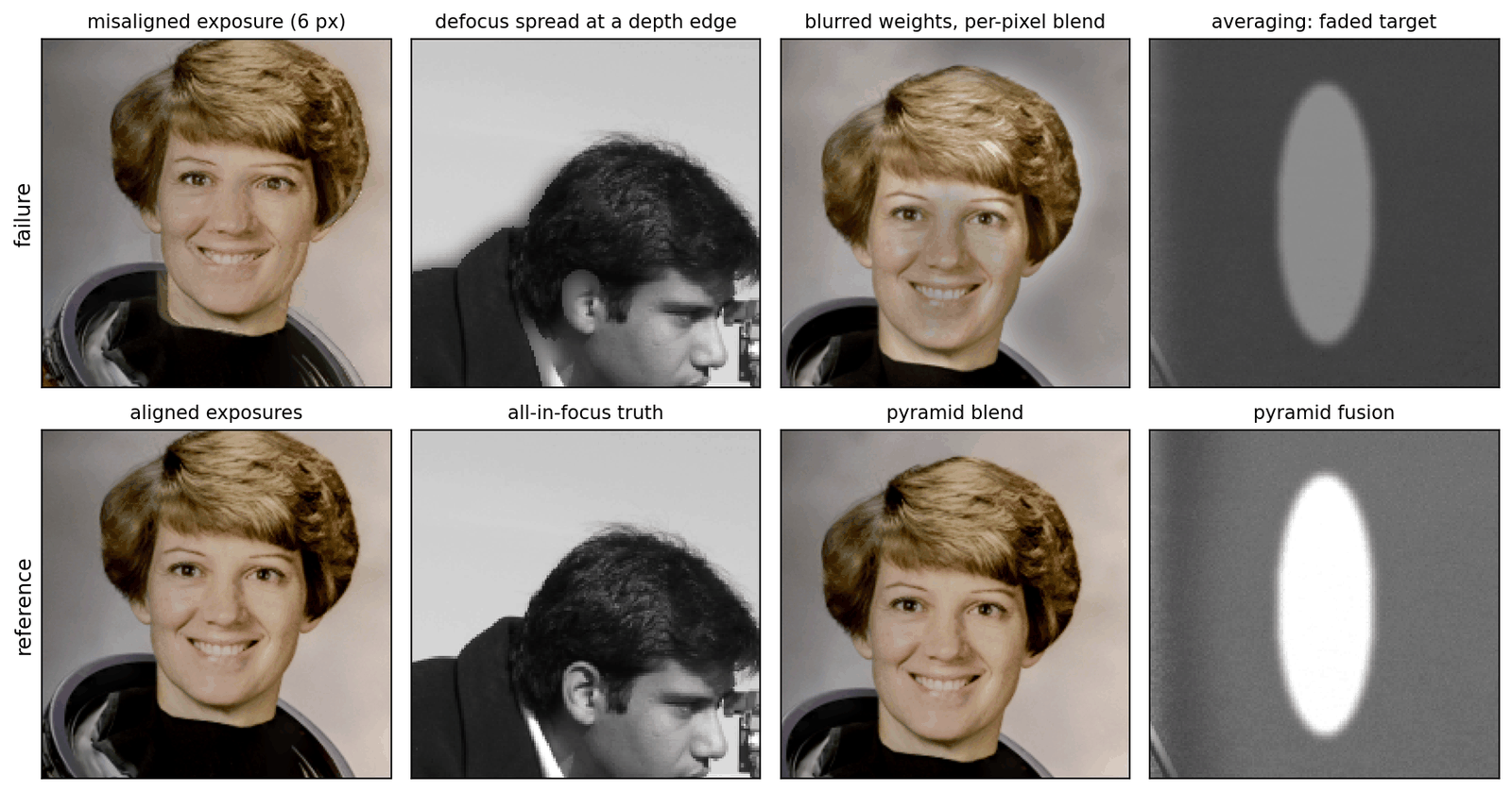
- Misregistration ghosts. A shift of a few pixels between sources turns edges into double edges (Figure 6, first column). In multi-exposure fusion, moving objects cause the same effect. Check alignment before blaming the fusion rule.
- Decision-map boundary artifacts. Near depth edges, the real blur of the foreground spills over the background, so neither source is sharp and any binary decision leaves a soft ring or a blocky edge (second column). Hard switches also show small seams where the map is wrong.
- Halos. Weights that are smoothed too much, or a base layer fused at too fine a scale, create bright or dark bands along strong edges (third column) [5]. Multi-scale blending can reduce them, but a pyramid that is too shallow brings back seams and low-frequency errors (Exercise 4).
- Washed-out thermal targets. Averaging, or a loss that weights the visible source heavily, halves the contrast of warm targets (fourth column); the opposite error makes the background look like an infrared image, flat and textureless.
- Color shifts. A common way to handle color is to fuse only the luminance (for example the Y channel of YCbCr) and to combine or copy the chroma separately, as DeepFuse does for exposures [31]. Where the fused luminance differs a lot from the source whose chroma is used, for example a bright thermal target on a dark visible background, the colors no longer fit and look washed out or tinted. For exposure stacks, selecting pyramid coefficients instead of blending them produced color shifts in the comparison of Mertens et al. [5].
- Noise amplification. Max-abs selection and gradient losses prefer strong high frequencies, and noise can dominate high-frequency responses in a dark visible image, so a fused night image can look sharper but noisier than either source. This is also why EN and SF reward such results.
- Metric gaming. A method tuned to EN, SF or SD can produce exactly the artifacts above while reporting better numbers (the toy of Figure 5).
Modern view
Surveys. Six surveys together cover the field:
- Ma, Ma and Li (Information Fusion 2019) [3] review classical and early deep infrared–visible fusion, introduce registration as a prerequisite, summarize applications and evaluation metrics, and compare eighteen methods with nine metrics. Takeaway: a reference point for classical methods and their evaluation habits before deep learning took over.
- Liu et al. (Information Fusion 2018) [1] wrote an early review (2018) of deep learning for pixel-level fusion across tasks. They list the difficulties of conventional fusion (hand-designed activity measures and fusion rules) and argue that learned features can replace them, grouping the early methods (CNNs, convolutional sparse representation, stacked autoencoders) into generic frameworks.
- Zhang and Demiris (TPAMI 2023) [35] review deep visible–infrared fusion by architecture (CNN-, autoencoder-, GAN- and transformer-based), with datasets and evaluation methods. Takeaway: deep methods have become the dominant approach for the task.
- Liu et al. (TPAMI 2025) [2] organize more than 180 learning-based infrared–visible methods along three dimensions, data compatibility (registration), fusion (architectures and losses) and task adaptation (detection, segmentation), and compare them on registration, fusion and downstream tasks.
- Zhang (TPAMI 2022) [50] surveys deep multi-focus fusion (methods, datasets, metrics) and compares deep and conventional methods experimentally.
- Xu et al. (Remote Sensing 2022) [51] review multi-exposure fusion for static and dynamic scenes and compare 18 methods with nine metrics.
Optional: The infrared–visible fusion survey of Liu et al. (in the Paper guides). How its taxonomy is built, how to read its comparison tables, and what it lists as open problems.
State of the art (2023–2026). Four trends stand out. First, fusion is increasingly judged by downstream tasks: methods are trained with detection or segmentation losses, benchmarks such as M3FD and FMB carry labels, and the fusion loss itself can be learned from the task loss [27], [28], [40]. Second, generative priors and language have entered: diffusion-based fusion without task-specific training [41], self-supervised training from imaging priors [52], and text-guided fusion that also handles degraded sources [42]. Third, registration is moving inside the model, with joint registration–fusion networks for unaligned infrared–visible pairs [43], [44]. Fourth, video fusion is starting: a CVPR 2026 work introduces M3SVD, 220 synchronized and registered infrared–visible videos with 153,797 frames, and a model whose bi-temporal attention mitigates the temporal inconsistency of frame-by-frame image fusion [53]. For multi-focus fusion, a 2020 benchmark study found that deep methods trained on simulated data did not generalize well to challenging real pairs, while conventional methods remained competitive [7]. Treat claims of large improvements with care, and check which metrics they rest on.
Open problems.
- Evaluation. There is still no metric, or set of metrics, that agrees with human judgment and with task performance; the 2025 survey names better evaluation metrics as an essential direction [2].
- Real misalignment and degradations. Most methods assume registered, clean sources. Benchmarks with registration ground truth, and fusion that is robust to noise, blur, low light and adverse weather in either source, are open [2], [42].
- Real defocus. Training data that reproduces the defocus spread effect, and methods that handle depth edges, are needed for multi-focus fusion to generalize [6], [7].
- Efficiency. Many recent networks are large; fusion on drones, cars and handheld devices needs lightweight, hardware-friendly designs [2] (see DLCV 09C for the general techniques).
- Video. Research has fused images rather than videos, largely because large synchronized multi-sensor video datasets were missing [53]; temporal consistency at low cost is open.
Key takeaways
- Choose what each source should contribute before selecting a fusion rule.
- Averaging can weaken source-specific features; weights should reflect useful information.
- Multi-scale blending separates fine-detail selection from coarse brightness blending, reducing seam risk.
- Without a unique fused target, training losses encode the desired answer and its compromises.
- Registration errors create ghosts; inspect boundaries, halos, colors, noise and source-specific targets.
- Use several metric families, crops and task results; a high score can reward noise or copying one source.
Exercises
- Contrast under averaging. A warm target has intensity in the infrared image and in the visible one, on a background of intensity in both. (a) Show that the average has target contrast and that any per-pixel weighted average with weights gives . (b) In our toy, the person contrast of the average is 0.257 and that of pyramid fusion 0.513. Which weight on the infrared source does pyramid fusion behave like on the target, and why does it achieve this without darkening the visible texture elsewhere?
Hint
(a) , using . (b) 0.513 is about twice 0.257, so on the target pyramid fusion behaves like . It can do so because the weights are not global: the coarse base takes the brighter source (the infrared target), while the fine levels take whichever detail is stronger, which is the visible texture away from the target. A global weight would have to trade the two against each other.
- Focus window and cleaning. In the multi-focus snippet, vary the focus-measure smoothing and the median window ( means no cleaning), always followed by the soft blend with a Gaussian of standard deviation 2. Report PSNR. Which setting wins, and why might the answer differ on real photographs?
Hint
In our run all settings lie between 39.43 and 40.05 dB; the best is with no median cleaning (40.05 dB), and the largest window, , is the worst for every (about 39.4–39.5 dB). Without cleaning, the soft blend mixes A and B in the speckled flat regions, which averages their independent noise and slightly raises PSNR there; a large median window misplaces the map near the boundary of the disk. On real photographs, uncleaned speckle shows up as visible blotches where the sources differ (noise, small misalignment, the defocus spread effect), so cleaning usually matters more for appearance than for PSNR on a toy.
- Area-based selection. Replace
pick_strongerin the pyramid snippet by a rule that compares local energies: smooth and with a Gaussian of standard deviation and choose the coefficient whose energy is larger. Try and compare with the per-coefficient rule.
Hint
Use ndi.gaussian_filter(p**2, s). In our run PSNR rose from 37.60 dB (per coefficient) to 39.14, 39.42 and 39.62 dB for , close to the decision map. Smoothing the activity makes neighboring coefficients take the same decision, which is what the area-based rule and consistency verification of Li et al. aim for: in multi-focus fusion, focus is a property of regions, not of single coefficients.
- Pyramid depth and quality measures in exposure fusion. (a) Rerun exposure fusion with pyramids of levels ( is the per-pixel blend) and report the well-exposed fraction; look at the images. (b) Use one quality measure at a time (contrast, saturation or well-exposedness only) at full depth. What do you observe?
Hint
(a) In our run the fraction was 72.3% for , then 72.2%, 70.9%, 69.6% and 68.5% for , and 73.8% for ; the mean absolute difference from the 9-level result was still 0.068 at . Shallow pyramids keep seams and low-frequency brightness errors, because the coarsest levels, where the weights are blended most smoothly, are missing; the result changes a lot even between 7 and 9 levels on a 512-pixel image. (b) Well-exposedness alone gave the highest fraction (77.5%), contrast alone 69.1% and saturation alone 71.5%. Mertens et al. also found that well-exposedness by itself gives fairly good images; contrast and saturation matter for detail and color, which this count does not measure.
- How noise inflates spatial frequency. Let where is independent zero-mean noise with variance at every pixel. (a) Show that the expected grows by about . (b) Check it on the toy: add noise with to the average and compare the measured SF with .
Hint
(a) A horizontal difference of is the difference of plus , whose variance is and which is uncorrelated with ; so , the same for CF, and . (b) In our run (with a different random seed from the snippet), the measured and predicted SF were 0.0528 and 0.0528 for , 0.0871 and 0.0871 for 0.04, and 0.1631 and 0.1637 for 0.08; the small gap at 0.08 comes from clipping to . EN rose from 6.69 to 6.99, 7.20 and 7.49 bits.
- Mutual information rewards copying. (a) Show that if , then , where is the entropy of the binned image. (b) Verify it on the toy with 64 bins. (c) Compute the MI score of the average and of the visible image with 16, 64 and 256 bins. Does the ranking depend on the bin count? Does the value?
Hint
(a) , because knowing removes all uncertainty about . (b) In our run bits and bits, which add up to 5.723, the MI score of “visible only” in the snippet. (c) The average scored 2.64, 4.33 and 5.00 bits and the visible image 3.42, 5.72 and 7.82 bits: the ranking stayed, but the values more than doubled from 16 to 256 bins for the visible image, so MI values from papers that use different bin counts or implementations cannot be compared.
References
- Y. Liu, X. Chen, Z. Wang, Z. J. Wang, R. K. Ward and X. Wang, “Deep learning for pixel-level image fusion: Recent advances and future prospects,” Information Fusion, vol. 42, pp. 158–173, 2018. doi
- J. Liu, G. Wu, Z. Liu, D. Wang, Z. Jiang, L. Ma, W. Zhong, X. Fan and R. Liu, “Infrared and visible image fusion: From data compatibility to task adaption,” IEEE Transactions on Pattern Analysis and Machine Intelligence, vol. 47, no. 4, pp. 2349–2369, 2025. doi arXiv
- J. Ma, Y. Ma and C. Li, “Infrared and visible image fusion methods and applications: A survey,” Information Fusion, vol. 45, pp. 153–178, 2019. doi
- P. E. Debevec and J. Malik, “Recovering high dynamic range radiance maps from photographs,” in Proc. SIGGRAPH, 1997, pp. 369–378. doi
- T. Mertens, J. Kautz and F. Van Reeth, “Exposure fusion: A simple and practical alternative to high dynamic range photography,” Computer Graphics Forum, vol. 28, no. 1, pp. 161–171, 2009. doi
- S. Xu, X. Wei, C. Zhang, J. Liu and J. Zhang, “MFFW: A new dataset for multi-focus image fusion,” arXiv:2002.04780, 2020. arXiv
- X. Zhang, “Multi-focus image fusion: A benchmark,” arXiv:2005.01116, 2020. arXiv
- P. J. Burt and E. H. Adelson, “The Laplacian pyramid as a compact image code,” IEEE Transactions on Communications, vol. 31, no. 4, pp. 532–540, 1983. doi
- P. J. Burt and R. J. Kolczynski, “Enhanced image capture through fusion,” in Proc. 4th International Conference on Computer Vision (ICCV), 1993, pp. 173–182. doi
- P. J. Burt and E. H. Adelson, “A multiresolution spline with application to image mosaics,” ACM Transactions on Graphics, vol. 2, no. 4, pp. 217–236, 1983. doi
- H. Li, B. S. Manjunath and S. K. Mitra, “Multisensor image fusion using the wavelet transform,” Graphical Models and Image Processing, vol. 57, no. 3, pp. 235–245, 1995. doi
- S. Li, X. Kang and J. Hu, “Image fusion with guided filtering,” IEEE Transactions on Image Processing, vol. 22, no. 7, pp. 2864–2875, 2013. doi
- K. He, J. Sun and X. Tang, “Guided image filtering,” IEEE Transactions on Pattern Analysis and Machine Intelligence, vol. 35, no. 6, pp. 1397–1409, 2013. doi
- B. Yang and S. Li, “Multifocus image fusion and restoration with sparse representation,” IEEE Transactions on Instrumentation and Measurement, vol. 59, no. 4, pp. 884–892, 2010. doi
- M. Nejati, S. Samavi and S. Shirani, “Multi-focus image fusion using dictionary-based sparse representation,” Information Fusion, vol. 25, pp. 72–84, 2015. doi
- Z. Wang, A. C. Bovik, H. R. Sheikh and E. P. Simoncelli, “Image quality assessment: From error visibility to structural similarity,” IEEE Transactions on Image Processing, vol. 13, no. 4, pp. 600–612, 2004. doi
- X. Zhang, P. Ye and G. Xiao, “VIFB: A visible and infrared image fusion benchmark,” in Proc. IEEE/CVF Conference on Computer Vision and Pattern Recognition (CVPR) Workshops, 2020. CVF arXiv
- X. Zhang, “Benchmarking and comparing multi-exposure image fusion algorithms,” Information Fusion, vol. 74, pp. 111–131, 2021. doi arXiv
- A. M. Eskicioglu and P. S. Fisher, “Image quality measures and their performance,” IEEE Transactions on Communications, vol. 43, no. 12, pp. 2959–2965, 1995. doi
- G. Qu, D. Zhang and P. Yan, “Information measure for performance of image fusion,” Electronics Letters, vol. 38, no. 7, pp. 313–315, 2002. doi
- M. Hossny, S. Nahavandi and D. Creighton, “Comments on ‘Information measure for performance of image fusion’,” Electronics Letters, vol. 44, no. 18, pp. 1066–1067, 2008. doi
- C. S. Xydeas and V. Petrović, “Objective image fusion performance measure,” Electronics Letters, vol. 36, no. 4, pp. 308–309, 2000. doi
- G. Piella and H. Heijmans, “A new quality metric for image fusion,” in Proc. IEEE International Conference on Image Processing (ICIP), 2003, vol. 3, pp. III-173–176. doi
- Y. Han, Y. Cai, Y. Cao and X. Xu, “A new image fusion performance metric based on visual information fidelity,” Information Fusion, vol. 14, no. 2, pp. 127–135, 2013. doi
- K. Ma, K. Zeng and Z. Wang, “Perceptual quality assessment for multi-exposure image fusion,” IEEE Transactions on Image Processing, vol. 24, no. 11, pp. 3345–3356, 2015. doi
- Z. Liu, E. Blasch, Z. Xue, J. Zhao, R. Laganiere and W. Wu, “Objective assessment of multiresolution image fusion algorithms for context enhancement in night vision: A comparative study,” IEEE Transactions on Pattern Analysis and Machine Intelligence, vol. 34, no. 1, pp. 94–109, 2012. doi
- J. Liu, X. Fan, Z. Huang, G. Wu, R. Liu, W. Zhong and Z. Luo, “Target-aware dual adversarial learning and a multi-scenario multi-modality benchmark to fuse infrared and visible for object detection,” in Proc. IEEE/CVF Conference on Computer Vision and Pattern Recognition (CVPR), 2022, pp. 5802–5811. CVF arXiv M3FD
- J. Liu, Z. Liu, G. Wu, L. Ma, R. Liu, W. Zhong, Z. Luo and X. Fan, “Multi-interactive feature learning and a full-time multi-modality benchmark for image fusion and segmentation,” in Proc. IEEE/CVF International Conference on Computer Vision (ICCV), 2023, pp. 8115–8124. CVF arXiv
- Y. Zhang, Y. Liu, P. Sun, H. Yan, X. Zhao and L. Zhang, “IFCNN: A general image fusion framework based on convolutional neural network,” Information Fusion, vol. 54, pp. 99–118, 2020. doi
- H. Li and X.-J. Wu, “DenseFuse: A fusion approach to infrared and visible images,” IEEE Transactions on Image Processing, vol. 28, no. 5, pp. 2614–2623, 2019. doi arXiv
- K. R. Prabhakar, V. S. Srikar and R. V. Babu, “DeepFuse: A deep unsupervised approach for exposure fusion with extreme exposure image pairs,” in Proc. IEEE International Conference on Computer Vision (ICCV), 2017, pp. 4724–4732. doi CVF
- H. Xu, J. Ma, J. Jiang, X. Guo and H. Ling, “U2Fusion: A unified unsupervised image fusion network,” IEEE Transactions on Pattern Analysis and Machine Intelligence, vol. 44, no. 1, pp. 502–518, 2022. doi RoadScene
- L. Tang, J. Yuan and J. Ma, “Image fusion in the loop of high-level vision tasks: A semantic-aware real-time infrared and visible image fusion network,” Information Fusion, vol. 82, pp. 28–42, 2022. doi
- J. Ma, L. Tang, F. Fan, J. Huang, X. Mei and Y. Ma, “SwinFusion: Cross-domain long-range learning for general image fusion via Swin Transformer,” IEEE/CAA Journal of Automatica Sinica, vol. 9, no. 7, pp. 1200–1217, 2022. doi
- X. Zhang and Y. Demiris, “Visible and infrared image fusion using deep learning,” IEEE Transactions on Pattern Analysis and Machine Intelligence, vol. 45, no. 8, pp. 10535–10554, 2023. doi
- Y. Liu, X. Chen, H. Peng and Z. Wang, “Multi-focus image fusion with a deep convolutional neural network,” Information Fusion, vol. 36, pp. 191–207, 2017. doi
- K. Ma, Z. Duanmu, H. Zhu, Y. Fang and Z. Wang, “Deep guided learning for fast multi-exposure image fusion,” IEEE Transactions on Image Processing, vol. 29, pp. 2808–2819, 2020. doi
- Z. Zhao, H. Bai, J. Zhang, Y. Zhang, S. Xu, Z. Lin, R. Timofte and L. Van Gool, “CDDFuse: Correlation-driven dual-branch feature decomposition for multi-modality image fusion,” in Proc. IEEE/CVF Conference on Computer Vision and Pattern Recognition (CVPR), 2023, pp. 5906–5916. CVF arXiv
- J. Ma, W. Yu, P. Liang, C. Li and J. Jiang, “FusionGAN: A generative adversarial network for infrared and visible image fusion,” Information Fusion, vol. 48, pp. 11–26, 2019. doi · public article transcription
- H. Bai, J. Zhang, Z. Zhao, Y. Wu, L. Deng, Y. Cui, T. Feng and S. Xu, “Task-driven image fusion with learnable fusion loss,” in Proc. IEEE/CVF Conference on Computer Vision and Pattern Recognition (CVPR), 2025, pp. 7457–7468. CVF arXiv
- Z. Zhao, H. Bai, Y. Zhu, J. Zhang, S. Xu, Y. Zhang, K. Zhang, D. Meng, R. Timofte and L. Van Gool, “DDFM: Denoising diffusion model for multi-modality image fusion,” in Proc. IEEE/CVF International Conference on Computer Vision (ICCV), 2023, pp. 8082–8093. CVF arXiv
- X. Yi, H. Xu, H. Zhang, L. Tang and J. Ma, “Text-IF: Leveraging semantic text guidance for degradation-aware and interactive image fusion,” in Proc. IEEE/CVF Conference on Computer Vision and Pattern Recognition (CVPR), 2024, pp. 27026–27035. CVF arXiv
- D. Wang, J. Liu, X. Fan and R. Liu, “Unsupervised misaligned infrared and visible image fusion via cross-modality image generation and registration,” in Proc. International Joint Conference on Artificial Intelligence (IJCAI), 2022, pp. 3508–3515. doi arXiv
- L. Tang, Y. Deng, Y. Ma, J. Huang and J. Ma, “SuperFusion: A versatile image registration and fusion network with semantic awareness,” IEEE/CAA Journal of Automatica Sinica, vol. 9, no. 12, pp. 2121–2137, 2022. doi
- A. Toet, “The TNO multiband image data collection,” Data in Brief, vol. 15, pp. 249–251, 2017. doi
- L. Tang, J. Yuan, H. Zhang, X. Jiang and J. Ma, “PIAFusion: A progressive infrared and visible image fusion network based on illumination aware,” Information Fusion, vol. 83–84, pp. 79–92, 2022. doi MSRS
- Q. Ha, K. Watanabe, T. Karasawa, Y. Ushiku and T. Harada, “MFNet: Towards real-time semantic segmentation for autonomous vehicles with multi-spectral scenes,” in Proc. IEEE/RSJ International Conference on Intelligent Robots and Systems (IROS), 2017, pp. 5108–5115. doi
- X. Jia, C. Zhu, M. Li, W. Tang and W. Zhou, “LLVIP: A visible-infrared paired dataset for low-light vision,” in Proc. IEEE/CVF International Conference on Computer Vision (ICCV) Workshops, 2021, pp. 3496–3504. CVF arXiv
- J. Cai, S. Gu and L. Zhang, “Learning a deep single image contrast enhancer from multi-exposure images,” IEEE Transactions on Image Processing, vol. 27, no. 4, pp. 2049–2062, 2018. doi
- X. Zhang, “Deep learning-based multi-focus image fusion: A survey and a comparative study,” IEEE Transactions on Pattern Analysis and Machine Intelligence, vol. 44, no. 9, 2022. doi
- F. Xu, J. Liu, Y. Song, H. Sun and X. Wang, “Multi-exposure image fusion techniques: A comprehensive review,” Remote Sensing, vol. 14, no. 3, art. 771, 2022. doi
- Z. Zhao, H. Bai, J. Zhang, Y. Zhang, K. Zhang, S. Xu, D. Chen, R. Timofte and L. Van Gool, “Equivariant multi-modality image fusion,” in Proc. IEEE/CVF Conference on Computer Vision and Pattern Recognition (CVPR), 2024, pp. 25912–25921. CVF arXiv
- L. Tang, Y. Wang, M. Gong, Z. Li, Y. Deng, X. Yi, C. Li, H. Xu, H. Zhang and J. Ma, “VideoFusion: A spatio-temporal collaborative network for multi-modal video fusion,” in Proc. IEEE/CVF Conference on Computer Vision and Pattern Recognition (CVPR), 2026, pp. 19559–19569. CVF
- N. Yokoya, C. Grohnfeldt and J. Chanussot, “Hyperspectral and multispectral data fusion: A comparative review of the recent literature,” IEEE Geoscience and Remote Sensing Magazine, 2017. doi
- H. R. Sheikh and A. C. Bovik, “Image information and visual quality,” IEEE Transactions on Image Processing, 2006. doi
- H. Xu et al., “U2Fusion,” official implementation accompanying the TPAMI paper, 2022. code
- K. Simonyan and A. Zisserman, “Very deep convolutional networks for large-scale image recognition,” ICLR, 2015. arXiv
- J. Kirkpatrick et al., “Overcoming catastrophic forgetting in neural networks,” Proceedings of the National Academy of Sciences, 2017. doi
- Y. Zhang et al., “IFCNN,” official implementation and errata accompanying the Information Fusion paper, 2020. code
- K. He, X. Zhang, S. Ren and J. Sun, “Deep residual learning for image recognition,” CVPR, 2016. CVF
- J. Deng, W. Dong, R. Socher, L.-J. Li, K. Li and L. Fei-Fei, “ImageNet: A large-scale hierarchical image database,” CVPR, 2009. doi
- N. Silberman, D. Hoiem, P. Kohli and R. Fergus, “Indoor segmentation and support inference from RGBD images,” ECCV, 2012. project
- P. Dhariwal and A. Nichol, “Diffusion models beat GANs on image synthesis,” NeurIPS, 2021. arXiv
- J. Liu et al., “TarDAL,” official implementation accompanying the CVPR paper, 2022. code
- G. Jocher et al., “YOLOv5,” Ultralytics object-detection software, 2020 onward. code
- J. Ma et al., “FusionGAN,” official implementation accompanying the Information Fusion paper, 2019. code
- L. Tang, J. Yuan and J. Ma, “SeAFusion,” official implementation accompanying the Information Fusion paper, 2022. code
- T. Mertens, J. Kautz and F. Van Reeth, “Exposure Fusion,” in Proc. Pacific Graphics, 2007. paper · author project
Check your understanding
This tutorial has 6 exercises. Can you solve them without opening the hints?
Go to the exercises ↑Next DLCV 11 · 3D Reconstruction: From Multi-View Geometry to NeRF and Gaussian Splatting · 42 min