IT 01 · Entropy, Relative Entropy and Mutual Information
Needs: ML 01B · Probability and Information Theory
Navigate: this page and this track: Navigate: this page and this track
On this page
- What you’ll learn1 min
- The big picture2 min
- Random variables, outcomes and the probability model1 min
- Surprise becomes additive through a logarithm1 min
- Entropy bounds and the binary example1 min
- Joint entropy and the chain rule1 min
- Conditioning helps on average, not necessarily for every outcome1 min
- Relative entropy measures probability mismatch1 min
- Cross-entropy connects prediction and coding3 min
- Mutual information measures dependence2 min
- Data processing, invertibility and added randomness1 min
- Estimation requires more than an identity1 min
- Modern view1 min
- Key takeaways1 min
- Exercises1 min
- References
Information Theory
Explore this chapter 2 interactive experiments
Separate source uncertainty, transmitted information and channel capacity.
What you’ll learn
- Explain why a logarithm converts probability into an additive measure of surprise.
- Calculate entropy, conditional entropy, relative entropy and mutual information.
- Derive chain rules and identify the equality conditions in fundamental inequalities.
- Explain what processing can discard, preserve or add without confusing randomness with information.
- Check information identities using finite probability tables and complete CPU examples.
- Distinguish a population quantity, an empirical estimate and a learning objective.
The big picture
A sensor sends a sequence of measurements. Some values are predictable; others are surprising. A compressor benefits from predictability, while a receiver benefits from measurements that reduce uncertainty about something it wants to know. These two benefits are related but different. A stream can be highly random and contain almost no useful evidence about a scene.
This track follows Thomas M. Cover and Joy A. Thomas’s Elements of Information Theory, second edition [1]. Its quantities have operational roles: entropy will guide compression, mutual information will describe communication limits, and relative entropy will connect probability mismatch to extra description length and statistical discrimination. We begin with finite alphabets so every quantity can be checked by explicit summation.
The Stanford entropy notes [2] give an accessible companion treatment. We use explicit synthetic probability models so the definitions and numerical checks can be inspected directly.
How the track fits together
| Tutorial | Main question | Core second-edition chapters |
|---|---|---|
| IT 01 | what does information measure? | 1–2, basic tools from 17 |
| IT 02 | why do long sequences become predictable in aggregate? | 3–4 |
| IT 03 | how can descriptions become short without losing symbols? | 5, 13–14 |
| IT 04 | how much can a noisy channel communicate reliably? | 7 |
| IT 05 | what changes for continuous and Gaussian variables? | 8–9 |
| IT 06 | what rate is required when some distortion is allowed? | 10 |
| IT 07 | how do information measures support inference and decisions? | 6, 11–12, 16 |
| IT 08 | what changes with several users, constraints and learning? | 15, advanced tools from 17 |
This grouping covers the book’s main themes without pretending that every theorem fits into a short derivation. Work through definitions, then numerical checks, then proofs. If a calculation feels mysterious, make the probability table explicit before adding a neural estimator or a communication system.
Random variables, outcomes and the probability model
A random variable describes what could be observed before the observation is known. Its probabilities belong to a model of the experiment. The same observed value can be surprising under one model and ordinary under another.
Let take values in a finite alphabet . Write
Here is the random variable, is a possible outcome, is the set of outcomes, is its probability mass function, and denotes probability. A joint distribution assigns probabilities to pairs. Marginals come from summation:
Here is another finite random variable, is one of its outcomes, and is its marginal mass function. Conditional probabilities use when . Conditioning on an event with zero probability needs separate conventions and will not contribute to the finite sums below.
We use base-two logarithms unless explicitly stated otherwise. Results are then in bits. Natural logarithms give nats; dividing a value in nats by converts it to bits. A bit is a unit of information, not necessarily a literal stored binary digit in a particular file format.
Keep the experiment fixed while comparing distributions. If one model describes grayscale intensities and another describes whole images, their numerical entropies are not directly comparable. Changing the variable, alphabet, quantization or conditioning information changes the question.
Surprise becomes additive through a logarithm
An unlikely outcome brings more surprise. Two independent observations should bring the sum of their individual surprises. A logarithm makes this addition agree with probability multiplication.
Define the self-information of an outcome:
Here is the surprise associated with outcome under model . If independent outcomes have probabilities and , their joint probability is , and . This is why doubling the number of equally likely possibilities adds one bit rather than multiplying the information value.
An outcome with probability one has zero surprise. A probability- outcome has three bits. These statements describe the probability model before seeing the outcome; observing an unusual symbol does not by itself make that symbol intrinsically valuable.
If a model gives an observed outcome probability zero, its surprise is infinite. In a prediction application, that may indicate a model-support error: the model declared an actually possible event impossible. Adding a small numerical constant changes the model. It can be useful, but it must not be confused with evaluating the original distribution.
The expected surprise is entropy:
Here is the entropy of , and averages over its probability distribution. The convention follows by taking a limit; outcomes that never occur do not contribute to the average.
Entropy is therefore a property of a distribution, not of one realized sample. A rare outcome can have high surprise even when the average entropy is small. An image may contain a visually striking pattern and still be easy for a suitable probability model to predict.
Entropy bounds and the binary example
Uncertainty is zero when the outcome is certain. For a fixed number of possibilities, uncertainty is greatest when all are equally likely.
If an alphabet has possible values,
Here is the alphabet size. The lower bound is attained by a point mass; the upper bound is attained by the uniform distribution. If only outcomes have positive probability, the sharper bound uses .
For a binary variable with probability of outcome one,
Here is the binary entropy function and . It is symmetric around . Its maximum is one bit, and it approaches zero near either endpoint. A highly biased source is easier to predict than a fair source even though both use the same two-symbol alphabet.
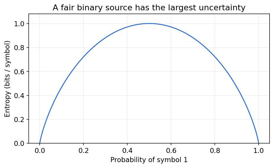
Entropy is concave in the distribution. Mixing two source distributions while hiding which one was selected cannot reduce entropy below their weighted average. Revealing that selection may remove part of the added uncertainty. This explains why mixtures often appear less predictable than their individual components.
The maximum-entropy bound can be proved using relative entropy to a uniform model; we will obtain it after defining divergence. The proof is useful because the same nonnegativity argument will also establish why conditioning reduces average entropy and why mutual information cannot be negative.
Joint entropy and the chain rule
Describing two variables can be cheaper than describing each independently. Once the first is known, shared structure may make the second easier to predict.
Joint entropy is
Here measures uncertainty about the pair . Conditional entropy is
Here is average remaining uncertainty about when is available. It weights the entropy of each conditional distribution by the probability of the corresponding .
Using gives
Every term refers to the same joint model. Taking the logarithm of the product creates two terms, and summing the first over leaves the marginal . This derivation explains the identity rather than merely providing a formula to memorize.
For a sequence :
Here is the number of variables and is the sequence index; the first term has no conditioning variables. This rule requires no independence assumption. Under independence, every conditional term equals its marginal entropy, so the joint entropy is the sum.
For an image, this distinction matters. A histogram describes marginal pixel frequencies but discards spatial dependencies. Two images with the same histogram can have very different predictability when nearby pixels are known. The sequence model determines whether those dependencies can shorten a description.
Conditioning helps on average, not necessarily for every outcome
Knowing another variable cannot make the optimal average prediction worse. But a particular observation can reveal that you are in an unusually uncertain situation.
Here the first inequality compares average conditional uncertainty with marginal uncertainty; the second follows from the chain rule. Equality holds when and are independent.
The phrase “on average” is essential. Suppose most days a sensor always outputs zero, but on rare diagnostic days it produces a fair binary outcome. Learning that today is a diagnostic day increases uncertainty relative to the marginal mixture. Learning the day type nevertheless lowers average uncertainty when averaged over both normal and diagnostic days.
Another distinction concerns more conditioning:
Here is additional information. This inequality concerns the entropies of one fixed joint distribution. It does not say that a finite neural network trained with extra inputs must generalize better. Optimization, limited data and spurious correlations can prevent a learned predictor from reaching the optimal conditional prediction.
Conditional entropy is nonnegative for finite variables. Later, differential entropy of continuous variables will behave differently. Do not transfer every finite-alphabet inequality to raw continuous entropy without checking its assumptions.
A numerical conditioning check
Make the diagnostic-day example explicit: let denote a diagnostic day with probability 0.1. On ordinary days ; on diagnostic days is a fair bit. Then the marginal probability of is , so bits.
Knowing that this is a diagnostic day raises uncertainty to bit. Averaging over all days instead gives bits. The conditioning inequality holds because it compares 0.1 with 0.286397, rather than comparing every individual conditional entropy with the marginal entropy. The day label removes bits on average.
Relative entropy measures probability mismatch
A probability model can waste description length by expecting the wrong outcomes. Relative entropy measures that mismatch in the direction of the distribution that actually generates observations.
Here and are probability mass functions on the same alphabet, and is their relative entropy, also called Kullback–Leibler divergence [1]. Terms with contribute zero. If but , the divergence is infinite.
Nonnegativity follows from concavity of the logarithm:
Here means expectation under . The first inequality is Jensen’s inequality; the final sum is at most one. Equality requires matching distributions. This proof also handles a model that places some probability outside the source support.
The direction matters. generally differs from . Divergence is not a metric: it does not obey all the requirements of a geometric distance, including symmetry and a general triangle inequality. Calling it a “distance” informally should not justify operations that require a genuine metric.
Compare a fair source with a model that gives probability to outcome one. The model is overconfident in one direction and pays for the frequent unexpected zeros. Reversing the distributions describes a different experiment and a different average penalty.
For a uniform distribution , expanding the divergence gives . Since it is nonnegative, the entropy upper bound follows. The equality condition also establishes why the uniform source uniquely maximizes entropy on a fixed finite alphabet.
Cross-entropy connects prediction and coding
Cross-entropy scores observations using a proposed probability model. It contains both the source’s unavoidable uncertainty and the cost of choosing an inaccurate model.
Here is cross-entropy, is the entropy of the true distribution, and supplies the predicted probabilities. Under idealized probability coding, is a description-length target. Actual codes also involve integer lengths, framing, model description and implementation overhead.
If stays fixed while parameters change , minimizing population cross-entropy also minimizes divergence. With data, the empirical mean negative log-probability estimates this objective:
Here is the number of observations, is observation , and denotes model parameters. The hat marks an empirical quantity. Its connection to the population average depends on how observations were sampled and whether they were reused to select the model.
A classifier applies the same idea conditionally to labels given features. A generative model applies it to observations or sequences. A low training value is evidence about fit to training observations, not automatically about future data. This distinction connects information theory to the evaluation rules in the ML/DL track.
When training code uses natural logarithms, the loss is in nats. Multiplying by a positive constant changes gradient scale but not the mathematical optimum. Comparing numerical losses across papers requires consistent units, normalization and prediction targets.
Worked example: one table, three information questions
Read the following table as a population model: each cell is the probability of observing that pair. It describes two fair bits that agree more often than they disagree.
| Joint probability | Row total | ||
|---|---|---|---|
| 0.4 | 0.1 | 0.5 | |
| 0.1 | 0.4 | 0.5 | |
| Column total | 0.5 | 0.5 | 1.0 |
Rows and columns sum to the marginal probabilities. Both marginals are fair, so bit. After observing , divide that row by its total 0.5: the conditional probabilities of are 0.8 and 0.2. The other row reverses them and has the same entropy.
Here is binary entropy, averages the two conditional rows, describes the pair, and is the reduction in uncertainty about either bit after seeing the other. All displayed values are in bits and rounded to six decimals; the code below computes them without rounding.
The same mutual information comes from comparing this joint table with the independent table, which has probability 0.25 in every cell. In agreeing cells the ratio is ; in disagreeing cells it is . Their weighted log ratios sum to 0.278072. A single cell’s log ratio can be negative even though the average divergence is nonnegative.
Now keep a fair one-bit source but predict probabilities 0.1 and 0.9. Its entropy stays one bit. Its cross-entropy becomes bits, leaving 0.736966 bits of model mismatch. The joint-table question measures dependence; this prediction question measures a wrong model. Both use divergence, but they compare different distributions.
This table also gives a simple interpretation for classification. Predicting is correct with probability 0.8, while the conditional distribution still contains 0.721928 bits of uncertainty. Accuracy counts correct decisions; entropy evaluates an entire predictive distribution. Neither number can be substituted for the other.
Code: exact finite-table checks
The following complete CPU example masks zero-probability terms instead of replacing them with a small constant. The helper functions also check that inputs are normalized probability arrays.
Code · Python · 36 lines
import numpy as np

def probability(a):
    a = np.asarray(a, dtype=float)
    assert np.all(a >= 0) and np.isclose(a.sum(), 1)
    return a

def entropy(a):
    a = probability(a)
    positive = a > 0
    return -np.sum(a[positive] * np.log2(a[positive]))

def divergence(p, q):
    p, q = probability(p), probability(q)
    assert p.shape == q.shape
    positive = p > 0
    if np.any(q[positive] == 0):
        return np.inf
    return np.sum(p[positive] * np.log2(p[positive] / q[positive]))

joint = probability([[0.4, 0.1], [0.1, 0.4]])
px, py = joint.sum(axis=1), joint.sum(axis=0)
independent = np.outer(px, py)
hx, hy, hxy = entropy(px), entropy(py), entropy(joint)
information = divergence(joint, independent)
print("H(X), H(Y), H(X,Y):", hx, hy, hxy)
print("H(Y|X), I(X;Y):", hxy - hx, information)
assert np.isclose(information, hx + hy - hxy)
assert np.isclose(divergence(independent, independent), 0)

p, q = probability([0.5, 0.5]), probability([0.1, 0.9])
cross = -np.sum(p * np.log2(q))
print("Source entropy / cross-entropy / mismatch:",
      entropy(p), cross, divergence(p, q))
assert np.isclose(cross, entropy(p) + divergence(p, q))
assert np.isinf(divergence(probability([0.5, 0.5]), probability([0, 1])))
The identities are checked on a specified population table. An empirical table built from finite observations adds estimation uncertainty; the algebra can be exact while the estimated value is statistically inaccurate.
Mutual information measures dependence
Two variables share information when knowing one changes what we expect about the other. Shared information is not limited to linear relationships.
Here is mutual information and is the product of the marginals. It is nonnegative, symmetric and zero exactly under independence. Its upper bound is the smaller of the two marginal entropies.
The divergence form asks how different the actual pair distribution is from an independent pair model. The entropy form asks how much average uncertainty one variable removes about the other. These viewpoints agree but emphasize different applications.
Correlation is narrower: zero correlation does not generally establish independence. Nonlinear dependencies can be strong even when a particular linear summary is zero. Conversely, estimating mutual information well in a high-dimensional space is often harder than estimating a correlation.
Conditional mutual information is
Here specifies the conditioning information. This quantity averages dependence within each conditional distribution. It is nonnegative, but it can be larger or smaller than unconditional .
For independent fair binary and , let be their parity. Unconditionally, tells us nothing about . Given , knowing determines . Thus the unconditional mutual information is zero and the conditional value is one bit. Conditioning can reveal dependencies rather than merely subtracting a fixed amount of information.
The information chain rule is
Here is a joint observation. The second term measures the extra information supplied by after is already available. Adding both unconditional values would double-count shared evidence or miss joint effects.
Mutual information as average predictive improvement
Expand the joint-distribution ratio using . The marginal factor cancels, giving
Here is the conditional distribution of after observing , the marginal prediction made without that observation, and divergence uses bits. This form expresses information as the average change from an unconditional prediction to a conditional one.
It also proves independence is the equality case. Every conditional divergence is nonnegative. Their weighted sum is zero only when each positive-probability leaves the prediction unchanged, which is exactly the finite-table independence condition. In the worked table, each conditional row differs from the fair marginal by the same divergence, .
Under logarithmic prediction loss, the best unconditional predictor pays , and the best conditional predictor pays . Their difference is mutual information. This is a population statement about optimal distributions: a fitted predictor can fail to realize the gain because it lacks data, capacity or an adequate optimization procedure. The derivation identifies the achievable predictive benefit and the reason its empirical estimate needs separate validation.
Data processing, invertibility and added randomness
Processing cannot create new evidence about an original source if it has access only to the current observation. It can add random variation, but variation is not the same as information about that source.
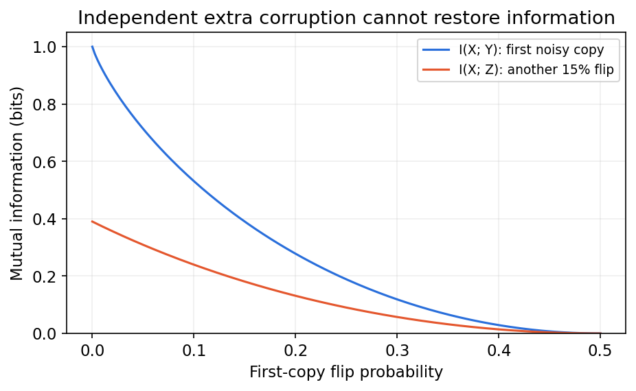
A Markov relation means
Here is generated from without extra access to . This condition implies the data-processing inequality:
The same appears on both sides. The inequality does not assert for arbitrary randomized processing. Adding independent noise can increase output entropy while decreasing information about the input.
A useful proof expands in two orders. The Markov relation makes . The other expansion includes nonnegative , leaving . Equality means that loses no relevant information about beyond what already supplies.
A deterministic transformation obeys because it merges possible outcomes. If it is one-to-one on the support, no uncertainty is lost. An invertible transformation of either variable also preserves mutual information. Compression through a many-to-one quantizer is different: it can discard dependencies.
Code: processing and parity
This second standalone example constructs the full three-variable probability table. It checks the processing inequality and the parity example without a fitted estimator.
Code · Python · 28 lines
import numpy as np

def entropy(p):
    p = np.asarray(p, dtype=float)
    assert np.all(p >= 0) and np.isclose(p.sum(), 1)
    q = p[p > 0]
    return -np.sum(q * np.log2(q))

def mutual(joint):
    return entropy(joint.sum(axis=1)) + entropy(joint.sum(axis=0)) - entropy(joint)

pxy = np.array([[0.4, 0.1], [0.1, 0.4]])
channel = np.array([[0.85, 0.15], [0.15, 0.85]])
pxyz = pxy[:, :, None] * channel[None, :, :]
pxz = pxyz.sum(axis=1)
print("Before / after processing:", mutual(pxy), mutual(pxz))
assert mutual(pxz) <= mutual(pxy) + 1e-12

parity = np.zeros((2, 2, 2))
for x in range(2):
    for y in range(2):
        parity[x, y, x ^ y] = 0.25
pxz, pyz = parity.sum(axis=1), parity.sum(axis=0)
pz = parity.sum(axis=(0, 1))
conditional = entropy(pxz) + entropy(pyz) - entropy(pz) - entropy(parity)
print("Parity I(X;Y) / I(X;Y|Z):",
      mutual(parity.sum(axis=2)), conditional)
assert np.isclose(conditional, 1)
When a reported estimated mutual information violates data processing, possible causes include sampling error, different estimator biases or a violated Markov assumption. The exact theorem has not ceased to hold.
Estimation requires more than an identity
Counting observed outcomes is easy. Deciding how much unobserved probability remains is not. Large alphabets and strong dependence can make information estimates fragile.
For counts among observations, the empirical distribution and plug-in entropy are
Here is the count of outcome , is the total sample count and hats denote estimates. Unobserved outcomes have empirical probability zero even if their true probability is positive.
For a fixed finite alphabet and independent sampling, the estimate converges under suitable conditions as samples grow. At small sample sizes, it typically underestimates entropy because the empirical distribution misses possible outcomes and appears too concentrated. Estimating a joint distribution requires covering a larger alphabet than either marginal alone.
Quantization also defines the variable. Binning a continuous feature into 8 levels and into 256 levels asks different finite-alphabet questions. Finer bins can add genuine resolution but also create more sparse cells. A smooth-looking information curve does not remove that trade-off.
The following standalone simulation checks average plug-in estimates for a known uniform source. It uses repeated synthetic samples, not a confidence claim from one draw.
Code · Python · 15 lines
import numpy as np

rng = np.random.default_rng(31)
alphabet = 20
truth = np.log2(alphabet)
for n in [40, 400, 4000]:
    estimates = []
    for _ in range(200):
        sample = rng.integers(alphabet, size=n)
        p = np.bincount(sample, minlength=alphabet) / n
        positive = p > 0
        estimates.append(-np.sum(p[positive] * np.log2(p[positive])))
    print("N:", n, "true entropy:", round(truth, 4),
          "mean estimate:", round(np.mean(estimates), 4))
assert abs(np.mean(estimates) - truth) < 0.02
For practical work, specify the sampling unit, feature transformations, estimator family, hyperparameter selection and uncertainty assessment. Repeated frames from one recording are not equivalent to independently sampled scenes. Evaluating an estimator on distributions with known information values is a useful first check.
Modern view
The basic quantities remain the same, but current applications often involve high-dimensional learned representations. The difficult step is frequently estimating or optimizing the quantity under a model, rather than writing its definition.
Butakov and colleagues [3] study mutual-information estimation through normalizing flows in NeurIPS 2024. Their method uses invertible transformations to simplify estimation while preserving the target information under stated assumptions. This illustrates a distinction: changing coordinates can help an estimator without creating information. The paper is an original method, not a survey or evidence that every neural estimator is unbiased.
Aubret, Matignon and Hassas’s 2023 survey [4] organizes intrinsic motivation through surprise, novelty and skill learning. It shows why an information quantity must be tied to its target: unpredictable observations, newly visited situations and controllable skills are different objectives. Our interpretation is that “maximize entropy” needs a specified variable and conditioning structure before it becomes a useful design rule.
El Gamal’s 2026 Information Theory and Statistical Learning manuscript [5] connects divergence-based objectives with predictive and generative modeling. It is a draft chapter proposed for a forthcoming third edition, not the published third edition or a replacement for the second-edition chapter numbers used here.
Open problems include reliable estimation in sparse high-dimensional spaces, comparison of estimators with different biases, dependence-aware evaluation and the relationship between a convenient information objective and the actual task. A learning method can improve an estimated lower bound without proving that its downstream decisions improved.
Use this chapter as a checklist when reading such claims: Which random variables? Which joint distribution? Which units? Is the number exact, estimated, bounded or optimized? What supports the conditional-independence assumption? These questions connect mathematical precision with useful empirical evidence.
Key takeaways
- Entropy is expected surprise under a probability distribution, not a property of one observed value.
- Chain rules account for shared structure and require no independence assumption.
- Conditioning reduces average uncertainty; individual conditional outcomes can behave differently.
- Relative entropy is directional, support-sensitive and nonnegative.
- Cross-entropy separates source uncertainty from model mismatch.
- Mutual information measures dependence; conditional dependence can differ sharply from unconditional dependence.
- Data processing limits evidence about a fixed source, while output randomness may increase.
- Empirical information estimates inherit sampling, quantization and model assumptions.
Exercises
- A three-symbol source has probabilities . Compute each outcome’s surprise and the entropy. Compare it with a uniform three-symbol source.
Hint
Average the logarithmic surprises with their probabilities.
- Construct a joint binary table with uniform marginals and mutual information zero, then another with mutual information one bit. Explain their conditional entropies.
Hint
Compare an outer product with a diagonal table.
- Expand for a uniform model on symbols and use nonnegativity to prove the entropy upper bound. State its equality condition.
Hint
The divergence becomes .
- Give a concrete model where for one value , while the average conditioning inequality still holds.
Hint
Use rare fair diagnostic days and common deterministic days.
- Extend the processing example with a third noisy channel. Check mutual information after every stage and identify the independence assumptions.
Hint
Multiply transition probabilities before summing out intermediate states.
- Repeat the entropy-estimation simulation with a larger alphabet and the same sample sizes. Describe which conclusions concern the estimator rather than the true entropy.
Hint
Record unseen-symbol counts as well as estimated entropy.
References
- T. M. Cover and J. A. Thomas, Elements of Information Theory, 2nd ed., Wiley, 2006, Chapters 1–2 and 17. Publisher book and contents.
- T. Weissman, “Entropy, Relative Entropy, and Mutual Information,” Stanford EE276 Lecture 2 notes, 2024. Primary lecture notes.
- I. D. Butakov, A. D. Tolmachev, S. V. Malanchuk, A. M. Neopryatnaya and A. A. Frolov, “Mutual Information Estimation via Normalizing Flows,” NeurIPS, 2024. Proceedings.
- A. Aubret, L. Matignon and S. Hassas, “An Information-Theoretic Perspective on Intrinsic Motivation in Reinforcement Learning: A Survey,” Entropy, 25(2), 327, 2023. Published survey.
- A. El Gamal, “Information Theory and Statistical Learning,” proposed textbook chapter, arXiv preprint, 2026. Draft and publication status.
Check your understanding
This tutorial has 6 exercises. Can you solve them without opening the hints?
Go to the exercises ↑Next IT 02 · Typical Sequences, AEP and Entropy Rates · 18 min