ML 11 · Evaluation, Efficiency and Deployment
Needs: ML 10 · Foundation Models and Vision–Language Learning
Navigate: this page and this track: Navigate: this page and this track
On this page
- What you’ll learn1 min
- The big picture1 min
- Start with a meaningful baseline1 min
- Data splits and leakage2 min
- Cross-validation3 min
- Metrics: a recap1 min
- Statistical significance and confidence intervals3 min
- Calibration: knowing when you might be wrong2 min
- Robustness and distribution shift2 min
- Efficiency: FLOPs, memory and latency2 min
- Deployment: export, compression and runtimes5 min
- Monitoring after deployment2 min
- Reproducibility and documentation2 min
- Modern view2 min
- Key takeaways1 min
- Exercises2 min
- Paper guides
- References
Machine Learning
Explore this chapter 1 interactive experiment
Apply one positive temperature to fixed validation logits and compare accuracy, log loss and squared probability error.
What you’ll learn
- Design baselines and data splits that support the deployment claim.
- Choose cross-validation and uncertainty estimates for the sampling structure.
- Distinguish accuracy, calibration and robustness under shift.
- Measure operations, memory and latency on the intended system.
- Validate exported models, monitor deployment and document reproducible runs.
The big picture
Training a model is the middle of a project, not the end. Before anyone relies on it, you need to answer four questions. Does it work on the cases it will really see? How sure are we of that number? Does it know when it is likely to be wrong? Does it fit the device, latency and budget it has to run on? After it ships, a fifth question appears: is it still working?
This chapter closes the ML track. It gathers the practical methodology from Goodfellow et al. [1, ch. 11] and the statistical-learning view of James et al. [2], and adds the engineering steps that turn a trained network into a dependable service. The task-specific metrics of vision (top-1, mAP, PSNR, FID and so on) are covered in DLCV 02 and DLCV 03; here we focus on what all tasks share.
Start with a meaningful baseline
Plain version. Before spending more compute, find out how well a simple method does on exactly the same split. The baseline tells you what the complicated model actually buys.
Good baselines for image tasks include: logistic regression on raw pixels or hand-designed features; a nearest-neighbor or SVM classifier; and a small linear head on frozen features from a pretrained model (see ML 10). Logistic regression learns a linear boundary; a support vector machine (SVM) maximizes a regularized margin; nearest neighbors compares examples directly; tree ensembles partition the feature space. The classical pattern-classification chapter, IP 13, develops these methods.
For reference, the binary linear SVM minimizes
where and are the weights and bias, is the -th feature vector, and trades margin width against training errors. The term is the hinge loss: it is zero for points on the correct side with margin at least 1 and grows linearly otherwise.
Code: baselines with preprocessing inside the pipeline
This example uses only bundled data. Model choice uses a validation split; the chosen model is evaluated on the test split once. Scaling and PCA are fitted inside each training pipeline, never on the full dataset.
Code · Python · 28 lines
from sklearn.datasets import load_digits
from sklearn.model_selection import train_test_split
from sklearn.pipeline import make_pipeline
from sklearn.preprocessing import StandardScaler
from sklearn.decomposition import PCA
from sklearn.linear_model import LogisticRegression
from sklearn.svm import SVC
from sklearn.metrics import accuracy_score, balanced_accuracy_score

X, y = load_digits(return_X_y=True)
Xa, Xt, ya, yt = train_test_split(X, y, test_size=.2, stratify=y, random_state=0)
Xtr, Xv, ytr, yv = train_test_split(Xa, ya, test_size=.25, stratify=ya, random_state=1)
models = {      # listed from simplest to most complex
    "linear": make_pipeline(StandardScaler(),
                           LogisticRegression(max_iter=2000)),
    "PCA + RBF SVM": make_pipeline(StandardScaler(), PCA(n_components=30),
                                  SVC(C=10, gamma="scale")),
}
scores = {}
for name, model in models.items():
    model.fit(Xtr, ytr)
    scores[name] = accuracy_score(yv, model.predict(Xv))
best = max(scores, key=scores.get)   # tie -> first listed, i.e. the simpler model
pred = models[best].predict(Xt)
print("validation:", scores)
print("selected:", best)
print("test accuracy:", accuracy_score(yt, pred))
print("test balanced accuracy:", balanced_accuracy_score(yt, pred))
On this split both candidates score exactly on validation (347 of 360 images). The rule “on a tie, prefer the simpler model” was fixed in advance, so the linear model is selected, and it scores accuracy and balanced accuracy on test. Two lessons hide in this tiny run. First, a tie-break rule is part of the protocol and should be written down before you look. Second, with 360 validation images a single image is worth percentage points, so many apparent “wins” in small experiments are noise; the section on confidence intervals makes this precise.
Data splits and leakage
Plain version. Make test data new in the way deployment will be new. Shared patients, scenes or time periods can inflate results when the claim concerns unseen groups or future data.
Choose the split unit from the claim
Images from one patient, one video, one production batch or one camera are correlated. Randomly splitting adjacent video frames puts almost the same picture in train and test. Ask what “new” means in deployment and split by that unit: by patient if the model will see new patients, by video if it will see new videos, by site if it will be installed in new hospitals, by time if it must predict the future.
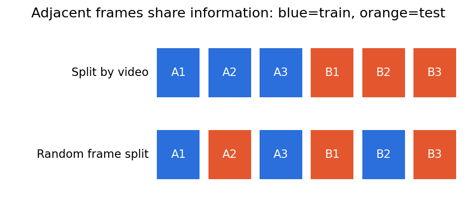
Stratification keeps class proportions similar across splits; it does not replace grouping. Deduplicate before splitting, and keep exact or near duplicates together. When the deployment population drifts over time, a time-based split (train on the past, test on the most recent period) is the honest choice.
The many faces of leakage
Leakage is any path by which information that would not be available at prediction time reaches the model or the model-selection process. Kapoor and Narayanan found leakage errors affecting 329 papers across 17 scientific fields that use ML, and propose a taxonomy of leakage types, among them missing train/test separation, preprocessing on the full dataset, duplicates, temporal leakage and illegitimate features [4]. The scikit-learn documentation lists the most common coding mistakes [3]. A practical checklist:
| Leak | Example | Fix |
|---|---|---|
| Preprocessing on all data | Fit StandardScaler, PCA or a vocabulary on train + test | Put preprocessing inside a Pipeline fitted on the training fold only |
| Correlated units | Frames of one video, slices of one scan, crops of one photo | Split by group |
| Duplicates | The same image scraped twice | Hash or embed and deduplicate before splitting |
| Temporal | Using next week’s data to predict this week | Time-ordered splits |
| Target proxy | A feature recorded after the outcome (e.g. “treatment given”) | Audit each feature’s timestamp |
| Test reuse | Tuning hyperparameters while watching the test score | Validation for decisions, test once |
The last row is subtle. Every time you look at the test score and change something, the test set becomes a little more like a validation set. Public benchmarks suffer from this at community scale.
Cross-validation
Plain version. Instead of one train/validation split, rotate: split the data into parts, train times, each time holding out a different part, and average. You use every example for evaluation once and you see how much the score varies.
K-fold and its variants
Partition the indices into disjoint folds . For each , train on all folds except and compute its error on . The cross-validation estimate is
where is the per-example loss (for example 0–1 error) and is the fold size. Common choices are or [2]. The variants differ only in how folds are formed:
- Stratified -fold keeps class proportions equal across folds; useful when classes are imbalanced.
- Group -fold assigns each group (patient, video, site) to exactly one fold, so no group appears in both training and held-out data.
- Time-series split always trains on earlier data and validates on later data.
- Leave-one-group-out is group -fold with one group per fold; useful with few groups.
The fold scores are not independent (training sets overlap), so the standard deviation across folds understates the true uncertainty. Treat it as a rough indication of stability, not as a formal confidence interval.
Code: what random K-fold does to grouped data
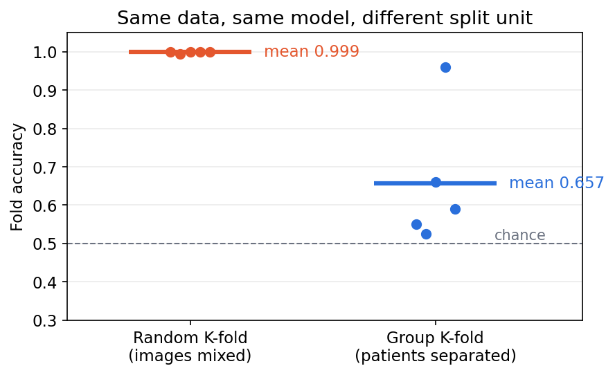
We simulate 40 patients with 25 images each. Every patient’s images share a “fingerprint” (patient-specific appearance), and the label is fixed per patient. The real class signal is weak.
Code · Python · 17 lines
import numpy as np
from sklearn.model_selection import KFold, GroupKFold, cross_val_score
from sklearn.ensemble import RandomForestClassifier

rng = np.random.default_rng(0)
n_groups, per_group = 40, 25                   # e.g. 40 patients, 25 images each
groups = np.repeat(np.arange(n_groups), per_group)
y = np.repeat(rng.integers(0, 2, n_groups), per_group)   # label fixed per patient
identity = rng.normal(size=(n_groups, 20))[groups]       # patient "fingerprint"
signal = 0.3 * y[:, None] * np.ones((1, 20))             # weak real class signal
X = identity + signal + 0.3 * rng.normal(size=(len(y), 20))

model = RandomForestClassifier(n_estimators=200, random_state=0)
random_cv = cross_val_score(model, X, y, cv=KFold(5, shuffle=True, random_state=0))
group_cv = cross_val_score(model, X, y, cv=GroupKFold(5), groups=groups)
print(f"random K-fold accuracy: {random_cv.mean():.3f} +/- {random_cv.std():.3f}")
print(f"group  K-fold accuracy: {group_cv.mean():.3f} +/- {group_cv.std():.3f}")
Output:
Code · 2 lines
random K-fold accuracy: 0.999 +/- 0.002
group  K-fold accuracy: 0.657 +/- 0.158
The random split reports near-perfect accuracy because the forest recognizes each patient’s fingerprint and copies that patient’s label. Group -fold, which matches the claim “works on new patients”, reports with large variation across folds. Neither number is wrong as arithmetic; only one answers the question.
Nested cross-validation
If you use cross-validation both to choose hyperparameters and to report performance, the reported number is optimistically biased: you picked the configuration that happened to look best on those folds. Varma and Simon demonstrated this with “null” data in which the two classes were statistically identical: after tuning an SVM by cross-validation, the CV error estimate fell below 30% on 38% of the simulated datasets, while the tuned classifiers were no better than chance on independent test data [5]; Cawley and Talbot showed that over-fitting the model-selection criterion can be as large as the differences between learning algorithms [6].
Nested CV fixes this with two loops. The outer loop holds out a fold for evaluation. Inside each outer training set, an inner CV selects hyperparameters. The outer fold is touched only to score the configuration the inner loop chose. In scikit-learn this is simply a GridSearchCV placed inside cross_val_score. The result estimates the performance of the whole procedure (including tuning), which is what you will run when you retrain.
For deep networks a full nested CV is often too expensive. The usual compromise is a single fixed train/validation/test split, a stated tuning budget for every method compared, and a test set that is opened once.
Metrics: a recap
Plain version. Decide what an error costs before choosing a number. One scalar rarely tells the whole story.
| Task | Useful measurements | Common trap |
|---|---|---|
| Classification | Per-class precision/recall, macro-F1, balanced accuracy, AUROC/AUPRC | Accuracy hides rare failures; PR curves depend on prevalence |
| Detection/segmentation | AP, IoU/Dice, boundary errors | Comparing different IoU thresholds or protocols |
| Retrieval | Recall@, mAP under a defined relevance set | Gallery duplicates inflate matches |
| Restoration | PSNR/SSIM, perceptual metrics, consistency with the observation | Plausible texture may not be true detail |
| Generation | FID/KID, coverage, conditional alignment, human study | Feature realism does not establish prompt fidelity |
| Video/geometry | Temporal consistency, task accuracy, geometric error | Good individual frames can hide inconsistent structure |
The definitions and pitfalls of classification metrics (confusion matrix, top-, ROC/PR curves) are worked through in DLCV 02, and those of detection (IoU, AP, COCO mAP) in DLCV 03. For generative models, FID compares Gaussian fits (means and covariances) of feature distributions; KID instead uses a kernel maximum-mean-discrepancy estimate that is unbiased, which makes it better behaved with small sample counts [7]. Neither is a universal measure of human preference. Always state the feature extractor, reference set, sample count, resolution and sampling settings.
With 1% positives, an always-negative classifier gets 99% accuracy and zero recall, so accuracy alone hides the failure. Precision also depends on prevalence. If only the class proportions change while the class-conditional input distributions and decision threshold stay fixed, recall and false-positive rate stay fixed, but precision changes [17]. This is the label-shift assumption; in a new hospital, camera or population, class-conditional appearances can also change, so all three rates must be remeasured rather than presumed stable.
Statistical significance and confidence intervals
Plain version. A test score is computed from a finite sample, so it would come out a little different on another sample. Report a range, not just a point, and compare two models on the same examples.
Standard error of an accuracy
If the test examples are independent and the model’s true accuracy is , the number of correct predictions is binomial, and the observed accuracy has standard error
Here is the fraction correct and is the 97.5th percentile of the standard normal distribution. For and , , so the interval is about percentage points. This normal approximation is poor when is very close to 0 or 1 or is small; Wilson or exact binomial intervals are better there. If test examples are grouped (several images per patient), the effective sample size is closer to the number of groups, and the interval must be computed by resampling groups.
The bootstrap
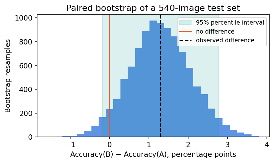
The bootstrap estimates the sampling distribution of any statistic by resampling the observed data with replacement [9]. Draw resamples of size , recompute the statistic on each, and take the 2.5th and 97.5th percentiles as an approximate 95% interval (the percentile interval). It works for metrics with no simple formula, such as macro-F1, AUROC or mAP.
To compare two models, use a paired bootstrap: resample example indices once, and evaluate both models on the same resample. Because the models usually fail on many of the same hard examples, pairing removes that shared variance and gives a much tighter interval for the difference than two separate intervals would.
McNemar’s test
For two classifiers evaluated on the same test set, only the examples where they disagree carry information about which is better. Let count examples model A gets right and B gets wrong, and the reverse. Under the null hypothesis that both models have the same error rate, each discordant example is equally likely to fall either way, so . The exact McNemar test computes a two-sided binomial p-value from that. Dietterich compared five tests for comparing learning algorithms and found that, for algorithms that can be run only once (typical for expensive models), McNemar’s test was the only one with acceptable type I error; when ten runs are affordable he recommended the 5×2 cross-validated t test [8].
Code: paired bootstrap and McNemar
Code · Python · 28 lines
import numpy as np
from scipy.stats import binomtest
from sklearn.datasets import load_digits
from sklearn.model_selection import train_test_split
from sklearn.pipeline import make_pipeline
from sklearn.preprocessing import StandardScaler
from sklearn.linear_model import LogisticRegression
from sklearn.svm import SVC

X, y = load_digits(return_X_y=True)
Xtr, Xte, ytr, yte = train_test_split(X, y, test_size=0.3, stratify=y, random_state=0)
a = make_pipeline(StandardScaler(), LogisticRegression(max_iter=2000)).fit(Xtr, ytr)
b = make_pipeline(StandardScaler(), SVC(C=10, gamma="scale")).fit(Xtr, ytr)
ca, cb = a.predict(Xte) == yte, b.predict(Xte) == yte    # per-example correctness

# 1) Percentile bootstrap: resample test examples with replacement.
rng = np.random.default_rng(0)
idx = rng.integers(0, len(yte), size=(10_000, len(yte)))
diff = cb[idx].mean(axis=1) - ca[idx].mean(axis=1)       # paired: same resample
lo, hi = np.percentile(diff, [2.5, 97.5])
print(f"accuracy A={ca.mean():.4f}  B={cb.mean():.4f}  n={len(yte)}")
print(f"B - A = {cb.mean() - ca.mean():+.4f}, 95% bootstrap CI [{lo:+.4f}, {hi:+.4f}]")

# 2) Exact McNemar test: only the discordant examples carry information.
n01 = int(np.sum(ca & ~cb))      # A right, B wrong
n10 = int(np.sum(~ca & cb))      # A wrong, B right
p = binomtest(n10, n01 + n10, 0.5).pvalue
print(f"discordant pairs: A-only={n01}, B-only={n10}, exact McNemar p={p:.4f}")
Output:
Code · 3 lines
accuracy A=0.9722  B=0.9852  n=540
B - A = +0.0130, 95% bootstrap CI [-0.0019, +0.0278]
discordant pairs: A-only=5, B-only=12, exact McNemar p=0.1435
The SVM is 1.3 points better, but the interval includes zero and McNemar’s p-value is . Only 17 of 540 images separate the two models, and 12 versus 5 is not unusual under a fair coin. With this test set, the honest conclusion is “B is probably at least as good; the evidence that it is better is weak.”
Other sources of variance
The test sample is not the only source of randomness. For a neural network, the random seed changes initialization, data order and augmentation; the data split itself is random; and some GPU kernels are nondeterministic. Bouthillier et al. modeled the whole benchmarking process and found that variance from data sampling, parameter initialization and hyperparameter choice markedly affects conclusions; they recommend randomizing as many of these sources as possible across repeated runs [10]. Practical rules:
- Run each configuration with several seeds (3–5 is common) and report mean and spread.
- Compare methods with paired tests on the same examples and splits.
- If you compare many models or many datasets, some will “win” by chance; adjust for multiple comparisons or confirm on a fresh set.
- Report effect sizes with intervals. A statistically significant difference can be practically irrelevant, and a large practical difference can be statistically unproven on a small set.
Calibration: knowing when you might be wrong
Plain version. A model’s confidence should match how often it is right. Among all predictions made with 80% confidence, about 80% should be correct. Accuracy and calibration are separate properties.
Measuring probability quality
Let be the predicted probability of class for example , and the one-hot label. Two proper scoring rules (scores minimized in expectation by the true probabilities) are:
where is the true class of example and is the number of classes. Some libraries divide the Brier score by ; say which convention you use.
The expected calibration error (ECE) groups predictions into bins by their top-class confidence and compares average confidence with accuracy in each bin:
where is the fraction correct in bin and the mean confidence there. A reliability diagram plots against per bin; a perfectly calibrated model lies on the diagonal. ECE is not a proper scoring rule and depends on the bin count and the bin scheme, so report it alongside NLL or Brier and a reliability diagram.
Temperature scaling
Guo et al. observed that modern deep networks, which are much larger than those of earlier decades, are often overconfident, and that a single scalar fix works surprisingly well [11]. Temperature scaling divides the logits by before the softmax:
softens overconfident predictions; sharpens underconfident ones. Because dividing all logits by the same positive number never changes which is largest, the predicted class (and so accuracy) is unchanged. must be fitted on a held-out calibration set, never on the test set. Later work by Minderer et al. found that the most recent image classifiers, notably non-convolutional ones such as Vision Transformers, are among the best calibrated, and that older trends such as calibration decaying under distribution shift are less pronounced for them [12].
Code: temperature scaling and what shift does to it
Code · Python · 41 lines
import numpy as np
from scipy.optimize import minimize_scalar
from scipy.special import log_softmax, softmax
from sklearn.datasets import load_digits
from sklearn.model_selection import train_test_split
from sklearn.neural_network import MLPClassifier

X, y = load_digits(return_X_y=True)
X = X / 16.0
Xa, Xte, ya, yte = train_test_split(X, y, test_size=0.4, stratify=y, random_state=0)
Xtr, Xcal, ytr, ycal = train_test_split(Xa, ya, test_size=0.3, stratify=ya, random_state=0)
net = MLPClassifier(hidden_layer_sizes=(128,), alpha=1e-6, max_iter=300,
                    random_state=0).fit(Xtr, ytr)

def logits(X):                       # log-probabilities = logits up to a constant
    return np.log(np.clip(net.predict_proba(X), 1e-12, 1.0))

def ece(prob, y, bins=10):
    conf, pred = prob.max(1), prob.argmax(1)
    edges = np.linspace(0, 1, bins + 1)
    total = 0.0
    for lo, hi in zip(edges[:-1], edges[1:]):
        m = (conf > lo) & (conf <= hi)
        if m.any():
            total += m.mean() * abs((pred[m] == y[m]).mean() - conf[m].mean())
    return total

def nll(T, z, y):
    return -log_softmax(z / T, axis=1)[np.arange(len(y)), y].mean()

T = minimize_scalar(nll, bounds=(0.05, 20), method="bounded",
                    args=(logits(Xcal), ycal)).x
print(f"fitted temperature T = {T:.2f}")
noise = np.random.default_rng(0).normal(size=Xte.shape)
for sigma in [0.0, 0.3, 0.6]:        # Gaussian pixel noise = a simple covariate shift
    Xs = np.clip(Xte + sigma * noise, 0, 1)
    z = logits(Xs)
    p_raw, p_ts = softmax(z, axis=1), softmax(z / T, axis=1)
    print(f"noise {sigma:.1f}: acc={(p_raw.argmax(1) == yte).mean():.3f}  "
          f"ECE raw={ece(p_raw, yte):.3f}  ECE scaled={ece(p_ts, yte):.3f}  "
          f"NLL raw={nll(1, z, yte):.3f}  NLL scaled={nll(T, z, yte):.3f}")
Output (scikit-learn may print a convergence warning, which is harmless here):
Code · 4 lines
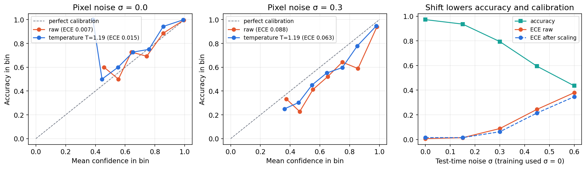
fitted temperature T = 1.19
noise 0.0: acc=0.972  ECE raw=0.007  ECE scaled=0.015  NLL raw=0.108  NLL scaled=0.110
noise 0.3: acc=0.794  ECE raw=0.088  ECE scaled=0.063  NLL raw=0.693  NLL scaled=0.639
noise 0.6: acc=0.435  ECE raw=0.380  ECE scaled=0.347  NLL raw=2.998  NLL scaled=2.598
Three observations. On clean data this small network is already well calibrated, and fitting on 324 calibration images slightly worsens ECE: a fix fitted on a small set can add noise. Under pixel noise the model becomes badly overconfident: at it is right 43.5% of the time while its confidence suggests far more. Temperature scaling fitted on clean data helps only a little under shift. This matches the large study by Ovadia et al., who found that the calibration of many uncertainty methods deteriorates as shift increases [16].
Optional: Temperature Scaling (in the Paper guides). Read the original figure, evidence, design choices and limitations.
Robustness and distribution shift
Plain version. New cameras, lighting or populations can change performance and calibration. Test relevant shifts rather than assuming deployment matches training.
Three kinds of shift
Write the joint distribution as , with the input and the label. Shifts are named by what changes between training () and deployment ():
- Covariate shift: while is unchanged. New camera, new lighting, new scanner.
- Label (prior) shift: while is unchanged. A disease becomes more common during an outbreak.
- Concept shift: itself changes. The definition of “spam” evolves.
Under pure covariate shift, the expected test loss can be rewritten as a weighted training loss, with importance weight . These weights are hard to estimate for images, but the identity explains why shift matters most where test inputs fall in regions with little training data. Under label shift, Lipton et al. showed that a fixed black-box classifier’s confusion matrix on held-out training data, combined with its prediction frequencies on unlabeled test data, is enough to estimate the new class priors and re-weight the model [17].
Benchmarks that probe shift
- ImageNet-C applies 15 corruption types (noise, blur, weather, digital) at several severities to ImageNet validation images, and ImageNet-P adds perturbation sequences; together they measure robustness to common corruptions rather than adversarial attacks [13]. Our pixel-noise sweep is a miniature version.
- ImageNetV2 re-created the ImageNet test set by following the original collection process as closely as possible. Accuracy dropped by 11–14% across many models, yet gains on the original test set translated into even larger gains on the new one, so the drop reflects slightly harder images rather than over-fitting to the reused test set [14]. Even a careful re-collection is a shift.
- WILDS gathers ten datasets with naturally occurring shifts, including tumor tissue from different hospitals, camera traps at new locations and satellite images from new countries, and reports a large gap between in-distribution and out-of-distribution performance that existing mitigation methods did not close [15].
The practical lesson: always add at least one shifted evaluation set built from the change you expect in deployment (new site, new device, later time), and report in-distribution and shifted results side by side.
Efficiency: FLOPs, memory and latency
Plain version. “Fast” and “small” each have several meanings. A model with fewer operations is not automatically quicker, and a model with fewer parameters does not automatically use less memory. Measure on the target device.
Counting operations
One multiply–accumulate (MAC) is a multiplication plus an addition, so 1 MAC ≈ 2 floating-point operations (FLOPs). For a fully connected layer with inputs and outputs, and a convolution with input channels, output channels, a kernel and an output:
per example (bias and activation costs are small). Libraries are inconsistent about whether they report MACs or FLOPs, so state which.
Why FLOPs do not equal speed
Dehghani et al. showed that common cost indicators (parameter count, FLOPs, throughput, latency) can disagree with each other and argued that reporting only one of them gives a misleading picture of efficiency [18]. The main reasons:
- Memory traffic. A layer whose weights must be read from memory for very little arithmetic is limited by memory bandwidth, not compute. A linear layer applied to a single example reads bytes of fp32 weights to perform FLOPs: 0.5 FLOPs per byte, far too little to keep a modern accelerator busy. Batching raises this ratio (called arithmetic intensity).
- Parallelism. Depthwise convolutions and many small layers have few FLOPs but use the hardware poorly.
- Kernel support. An operation without an optimized kernel on the target runtime may be slow regardless of its FLOP count.
Memory accounting
At inference, memory holds weights (), activations of the layers currently alive, workspace for kernels, and for autoregressive Transformers a KV cache that grows with context length and batch size. During training add gradients and optimizer states: Adam keeps two extra values per parameter, so an fp32 model with Adam needs roughly its weight memory before counting activations.
A latency protocol
Wall-clock latency depends on hardware, runtime, batch size, input resolution, numeric precision and thread settings, and the first calls are slower because of one-off initialization. A sound protocol:
- Fix and report device, runtime version, precision, batch size, input size and thread count.
- Run warm-up iterations and discard them.
- Time many runs and report percentiles (p50 and p90 or p99), not just the mean: users experience the tail.
- On GPUs, synchronize the device before stopping the timer, because kernels are launched asynchronously.
- Measure end to end (pre-processing, transfers, decoding) as well as the network alone.
A Pareto frontier contains the candidates for which no other candidate is at least as good on every axis (accuracy, latency, memory) and strictly better on one. Presenting the frontier makes trade-offs visible without inventing a single “best model”.
Deployment: export, compression and runtimes
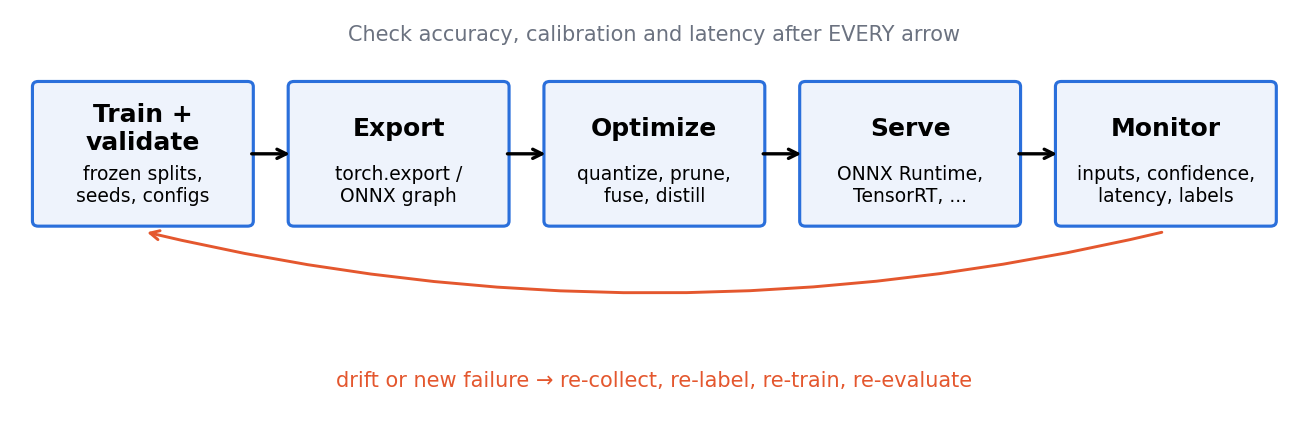
Plain version. Export, compression and runtime choices can change predictions and performance. Re-evaluate the artifact that will actually run on the target device.
Export and inference runtimes
Training code is written in a flexible, Python-driven framework. Deployment prefers a static description of the computation:
torch.exporttraces a PyTorch module ahead of time into anExportedProgram, a graph of tensor operations that can be serialized and executed with different inputs without the original Python class [19].- ONNX (Open Neural Network Exchange) is an open standard file format for ML models, so a model trained in one framework can be run by tools from others [20].
- ONNX Runtime is a cross-platform inference engine for ONNX models. It partitions the graph into subgraphs and hands each to a hardware-specific execution provider (for example CUDA, TensorRT, OpenVINO or CoreML) [21].
- NVIDIA TensorRT is an SDK that compiles models (from frameworks or ONNX) into optimized engines for NVIDIA GPUs, using layer fusion and reduced precisions such as FP16, BF16, FP8 and INT8 [22].
These runtimes gain speed by fusing operations, choosing fast kernels for the exact shapes and lowering precision. The same model can therefore give slightly different outputs on different runtimes. Compare exported and original outputs on a validation batch and re-measure accuracy after conversion.
Quantization
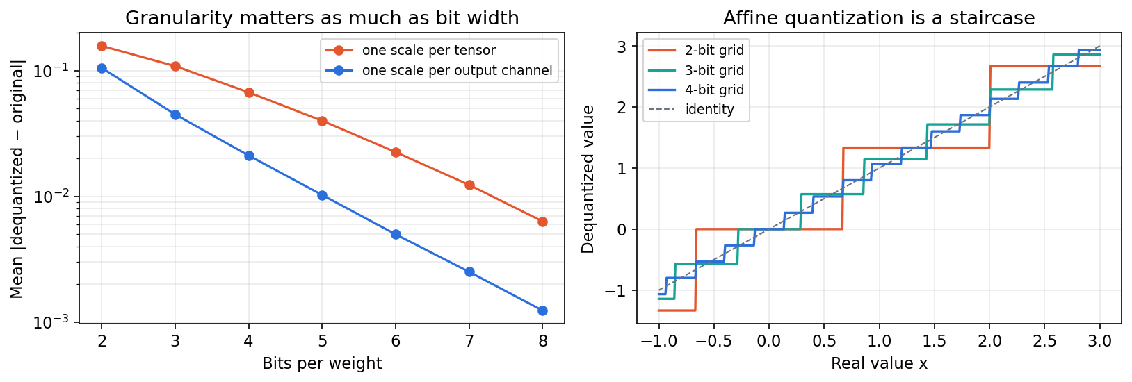
Quantization stores and computes with fewer bits. In the common affine (asymmetric) uniform scheme, a real value is mapped to an integer and back:
where is the bit width, the scale (the step between representable values), the integer zero point chosen so that the real value 0 is represented exactly, and the dequantized approximation. For a range that includes 0, and . The symmetric variant fixes and uses a signed range. The integer-arithmetic formulation of Jacob et al. showed how to run whole networks with 8-bit integer matrix multiplication and how to train for it [23].
Error comes from two sources: rounding inside the range (at most per value) and clipping outside it. Both depend on the granularity of the scale: one scale per tensor, per output channel, or per small group of weights. Nagel et al. give a practical guide covering these choices, post-training quantization (PTQ: calibrate ranges on a small representative dataset after training) and quantization-aware training (QAT: simulate rounding during training so the weights adapt) [24]. Gholami et al. survey the wider design space [25].
Code · Python · 21 lines
import numpy as np

def quantize(x, bits=8, axis=None):
    """Asymmetric (affine) uniform quantization, per tensor or per channel."""
    qmin, qmax = 0, 2**bits - 1
    lo = x.min(axis=axis, keepdims=True) if axis is not None else x.min()
    hi = x.max(axis=axis, keepdims=True) if axis is not None else x.max()
    lo, hi = np.minimum(lo, 0), np.maximum(hi, 0)      # keep 0 exactly representable
    s = (hi - lo) / (qmax - qmin)                       # scale
    z = np.round(qmin - lo / s)                         # zero point (integer)
    q = np.clip(np.round(x / s) + z, qmin, qmax)        # stored integers
    return s * (q - z)                                  # dequantized values

rng = np.random.default_rng(0)
# 64 output channels whose weight magnitudes differ by up to 100x
W = rng.normal(size=(64, 256)) * np.logspace(-2, 0, 64)[:, None]
for bits in [8, 4]:
    e_t = np.abs(quantize(W, bits) - W).mean()
    e_c = np.abs(quantize(W, bits, axis=1) - W).mean()
    print(f"{bits}-bit mean |error|: per-tensor {e_t:.5f}  per-channel {e_c:.5f}")
print("zero maps back to:", quantize(np.array([-1.0, 0.0, 3.0]))[1])
Output:
Code · 3 lines
8-bit mean |error|: per-tensor 0.00632  per-channel 0.00124
4-bit mean |error|: per-tensor 0.06718  per-channel 0.02112
zero maps back to: 0.0
When channels have very different ranges, one shared scale wastes most of the grid on the largest channel and rounds small channels coarsely. Per-channel scales cut the error about fivefold at 8 bits here. In large language models, a few outlier activation channels cause the same problem at a larger scale, which is what methods such as GPTQ (layer-wise error-compensating weight rounding) and AWQ (protecting salient weight channels identified from activations) address for 3–4-bit weight-only quantization [42], [43].
Pruning
Pruning removes weights, channels, attention heads or blocks that contribute little. Unstructured pruning zeros individual weights; it can remove a large fraction of parameters, as in Deep Compression, which combined pruning, weight sharing via quantization, and Huffman coding to shrink networks substantially [26]. But scattered zeros save time only if the runtime has sparse kernels for that pattern. Structured pruning removes whole channels or heads, producing smaller dense tensors that any runtime can exploit. Blalock et al. reviewed 81 pruning papers and found that inconsistent baselines and metrics made it hard to tell which methods actually work, and proposed a standardized benchmark [27]. Hoefler et al. survey sparsity in training and inference in depth [28].
Knowledge distillation
Distillation trains a small student to imitate a large teacher. Hinton et al. proposed matching the teacher’s softened output distribution [29]. With temperature , logits (teacher) and (student), softened probabilities , and weight :
The softened teacher distribution carries “dark knowledge” about which wrong classes are similar. The gradients of the soft term scale as , so multiplying by keeps the two terms balanced when changes [29]. Gou et al. organize later work by what is transferred (responses, intermediate features, relations between examples) and how (offline, online, self-distillation) [30]. A student inherits the teacher’s mistakes and biases as well as its skill.
Code: weight-only int8, latency and export
This sketch stores the weights of a small MLP as int8 with one scale per output channel and measures size and latency on the CPU. It uses only core PyTorch.
Code · Python · 53 lines
import io, time
import numpy as np
import torch
from torch import nn

torch.manual_seed(0)
model = nn.Sequential(nn.Linear(512, 2048), nn.ReLU(),
                      nn.Linear(2048, 2048), nn.ReLU(),
                      nn.Linear(2048, 10)).eval()
x = torch.randn(32, 512)

class Int8WeightLinear(nn.Module):
    """Weight-only int8 storage, symmetric per output channel."""
    def __init__(self, lin):
        super().__init__()
        w = lin.weight.detach()
        scale = w.abs().amax(dim=1, keepdim=True) / 127
        self.register_buffer("q", torch.round(w / scale).to(torch.int8))
        self.register_buffer("scale", scale)
        self.register_buffer("bias", lin.bias.detach().clone())
    def forward(self, x):                       # dequantize, then fp32 matmul
        return nn.functional.linear(x, self.q.float() * self.scale, self.bias)

int8 = nn.Sequential(*[Int8WeightLinear(m) if isinstance(m, nn.Linear) else m
                       for m in model]).eval()

def size_mb(m):
    buf = io.BytesIO()
    torch.save(m.state_dict(), buf)
    return buf.getbuffer().nbytes / 1e6

def latency_ms(m, x, warmup=10, runs=100):
    with torch.inference_mode():
        for _ in range(warmup):                 # first calls pay one-off costs
            m(x)
        times = []
        for _ in range(runs):
            t0 = time.perf_counter()
            m(x)
            times.append((time.perf_counter() - t0) * 1e3)
    return np.percentile(times, [50, 90]).round(2)

with torch.inference_mode():
    gap = (model(x) - int8(x)).abs().max().item()
    agree = (model(x).argmax(1) == int8(x).argmax(1)).float().mean().item()
print(f"fp32 file: {size_mb(model):.1f} MB  p50/p90 latency {latency_ms(model, x)} ms")
print(f"int8 file: {size_mb(int8):.1f} MB  p50/p90 latency {latency_ms(int8, x)} ms")
print(f"max |logit difference| = {gap:.4f}, top-1 agreement = {agree:.3f}")

# Ahead-of-time graph capture: a portable program, independent of this Python class.
exported = torch.export.export(model, (x,))
ops = [n.target for n in exported.graph.nodes if n.op == "call_function"]
print(type(exported).__name__, "->", [str(o).split(".")[1] for o in ops])
One CPU run (four threads) printed:
Code · 4 lines
fp32 file: 21.1 MB  p50/p90 latency [2.74 4.49] ms
int8 file: 5.3 MB  p50/p90 latency [ 9.23 11.06] ms
max |logit difference| = 0.0018, top-1 agreement = 1.000
ExportedProgram -> ['linear', 'relu', 'linear', 'relu', 'linear']
Your latencies will differ; the pattern is the point. The file is four times smaller and the outputs barely change. Yet the int8 version is slower, because it converts the weights back to fp32 on every call and then runs the same fp32 matrix multiplication. Lower precision becomes faster only when the runtime has integer (or low-precision) kernels for that operation, or when the workload is limited by memory bandwidth so that reading fewer bytes dominates. This is exactly the gap between “compressed” and “accelerated” that runtimes such as TensorRT, ONNX Runtime and PyTorch’s own torchao library [46] are built to close. The FLOP count of this MLP is MFLOPs per example, identical for both versions.
Monitoring after deployment
Plain version. A model can get worse without any code changing, because the data changes. Watch the inputs and outputs, collect fresh labels when possible, and decide in advance what triggers an investigation.
Sculley et al. describe how ML systems accumulate hidden “technical debt”: entangled features, undeclared consumers of predictions, feedback loops where the model’s outputs influence its future training data, and dependence on external data that changes without notice [33]. Paleyes et al. collected published deployment case studies and found problems at every stage of the workflow [39]. Useful signals, from cheapest to most informative:
- System health: latency percentiles, error rates, memory, throughput.
- Input statistics: image brightness, resolution, class of device, missing fields; compared with a reference window from training time.
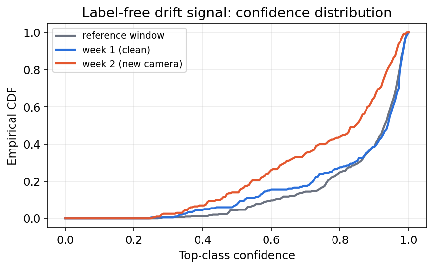
- Output statistics: distribution of predicted classes and of confidence. These need no labels.
- Delayed labels: a small, regularly labelled sample of live traffic gives the only direct estimate of accuracy.
To compare a live window with the reference, a two-sample test is a simple starting point. The Kolmogorov–Smirnov statistic for one-dimensional samples with empirical cumulative distribution functions and is
the largest vertical gap between the two curves. Rabanser et al. compared shift detectors and found that a two-sample test applied after reducing the inputs with a pre-trained classifier (for example to its softmax outputs) performed best across the shifts they studied [32].
Code · Python · 22 lines
import numpy as np
from scipy.stats import ks_2samp
from sklearn.datasets import load_digits
from sklearn.model_selection import train_test_split
from sklearn.linear_model import LogisticRegression

X, y = load_digits(return_X_y=True)
X = X / 16.0
Xtr, Xlive, ytr, ylive = train_test_split(X, y, test_size=0.5, random_state=0)
Xtr, Xref, ytr = Xtr[:600], Xtr[600:], ytr[:600]   # reference window from training time
clf = LogisticRegression(max_iter=2000).fit(Xtr, ytr)
ref_conf = clf.predict_proba(Xref).max(1)     # label-free signal: top-class confidence

rng = np.random.default_rng(0)
for name, noise in [("week 1 (clean)", 0.0), ("week 2 (new camera)", 0.25)]:
    batch = rng.choice(len(Xlive), 200, replace=False)
    Xb = np.clip(Xlive[batch] + noise * rng.normal(size=Xlive[batch].shape), 0, 1)
    conf = clf.predict_proba(Xb).max(1)
    stat, p = ks_2samp(ref_conf, conf)
    acc = (clf.predict(Xb) == ylive[batch]).mean()   # usually NOT available live
    print(f"{name}: mean confidence {conf.mean():.3f}, KS={stat:.3f}, p={p:.2g}, "
          f"(hidden) accuracy {acc:.3f}")
Output:
Code · 2 lines
week 1 (clean): mean confidence 0.846, KS=0.089, p=0.28, (hidden) accuracy 0.950
week 2 (new camera): mean confidence 0.757, KS=0.277, p=1.3e-08, (hidden) accuracy 0.885
The confidence distribution flags week 2 without a single label, and the hidden accuracy confirms that something real happened. A detector says that the data changed, not whether accuracy fell: harmless shifts also trigger it, and with large windows even tiny changes become “significant”. Use it to trigger investigation and labelling, not automatic retraining.
Reproducibility and documentation
Plain version. Someone else (including you in six months) should be able to rerun your experiment and get the same numbers, and a reader should be able to tell what the model is for and where it should not be used.
Making runs repeatable
Fix and record random seeds for every library, but know their limits: the PyTorch documentation states that completely reproducible results are not guaranteed across releases, commits or platforms, and recommends seeding, torch.use_deterministic_algorithms(True) and disabling cuDNN benchmarking when bit-exact repetition matters [34]. Beyond seeds, record:
- the dataset version, split IDs (the actual lists of example IDs) and deduplication rule;
- preprocessing and augmentation code, pretrained checkpoint and its source;
- the full configuration (optimizer, schedule, stopping rule), software environment and hardware;
- every validation decision made, and the single final test evaluation.
The NeurIPS 2019 reproducibility program, reported by Pineau et al., introduced a code-submission policy, a community reproducibility challenge and a checklist covering exactly these items [37].
Documenting models and data
Model cards are short documents that accompany a trained model and report its intended use, the evaluation data, performance broken down by relevant groups and conditions, and known limitations [35]. Datasheets for datasets ask dataset creators to document motivation, composition, collection process, preprocessing, recommended uses and maintenance [36]. Both make the evaluation decisions in this chapter visible to the people who will rely on them.
A capstone experiment
Choose one task with a modest, legally usable dataset. Define the deployment population and the split unit. Compare three candidates: a classical baseline, frozen pretrained features with a small head, and one fine-tuned network. For each, report the test metric with a bootstrap interval, a paired comparison against the best baseline, a reliability diagram, results on one shifted set, and latency percentiles on the target device. Write a one-page model card. Open the final test set once; if it reveals a failure and you revise the model, treat the old result as development evidence and obtain a fresh evaluation for the revised claim.
Modern view
The engineering of evaluation and deployment is now a research field in its own right. Several surveys and reviews map it.
Leakage and reproducibility. Kapoor and Narayanan’s review of ML-based science documents leakage in 329 papers across 17 fields and proposes “model info sheets” that make authors argue why their train/test separation is valid [4]. Combined with the variance study of Bouthillier et al. [10] and the NeurIPS reproducibility program [37], the consensus is that most over-optimistic results come from protocol errors, not from exotic statistics.
Uncertainty and calibration. Gawlikowski et al. survey uncertainty estimation in deep networks: they separate reducible model (epistemic) uncertainty from irreducible data (aleatoric) uncertainty, organize methods into deterministic networks, Bayesian networks, ensembles and test-time augmentation, and review calibration methods and their practical limits [38]. Ovadia et al. add the empirical warning that post-hoc calibration falls short under shift while methods that marginalize over models, such as ensembles, hold up better [16].
Deployment in practice. Paleyes et al. survey published case studies, map the challenges onto the stages of the deployment workflow and show that practitioners hit problems at every stage [39], extending the technical-debt view of Sculley et al. [33].
Compression. Cheng et al. give the classic overview of pruning, low-rank factorization, compact convolutions and distillation for CNNs [31]; Gholami et al. [25] and Nagel et al. [24] focus on quantization; Hoefler et al. on sparsity [28]; Gou et al. on distillation [30]. For large language models, Zhu et al. survey quantization, pruning, distillation and low-rank methods specific to models with billions of parameters [41]. A visible 2023–2026 trend is that weight-only quantization to 4 bits (GPTQ [42], AWQ [43]) and low-precision formats such as FP8 have moved from papers into production toolkits: TensorRT lists FP8, INT8, FP4 and INT4 among its supported precisions [22], and PyTorch’s quantization tooling is consolidating in the torchao library [46].
Holistic evaluation. For foundation models, HELM evaluates many models on many scenarios and on several metrics at once (accuracy, calibration, robustness, fairness, bias, toxicity and efficiency) and argues that a single leaderboard number hides these trade-offs [40]. The same multi-metric habit applies to vision models.
Scaling. Scaling laws fit empirical relationships among model size, data, compute and loss. Hoffmann et al. found that, for a fixed compute budget, language models should scale parameters and training tokens roughly equally [44]; Zhai et al. studied how ViT accuracy scales with model size, data and compute [45]. Fitted constants from one domain should not be copied into another; the transferable lesson is to report the compute and data behind every result.
Open problems. Evaluation sets leaking into web-scale pretraining data (contamination) is hard to rule out; calibration under unknown shift remains unsolved; latency claims rarely transfer between hardware generations; and evaluation of generative and interactive systems (see DLCV 13) still lacks agreed protocols.
Key takeaways
- Split by what will be new at deployment and fit preprocessing within each training fold.
- Use grouped or temporal folds for dependent data; separate model selection from reported evaluation.
- Compare models on paired examples and estimate uncertainty using the actual independent sampling unit.
- Calibration differs from accuracy; temperature scaling can help on matched data but does not guarantee calibration after shift.
- Operation counts, parameter counts, memory and latency measure different costs; benchmark the complete target pipeline.
- Re-evaluate after export or compression, monitor changing data, and record versions, protocols and intended use.
Exercises
- Leakage audit. A colleague fits PCA on all 1,797 digits, then splits into train and test and reports test accuracy. Explain the leak, and why it exists even though PCA never sees labels. How would you fix the code?
Hint
The principal directions are computed using the test images, so the representation is tuned to the test distribution. Put PCA inside a Pipeline so it is fitted only on each training fold. The bias is often small for PCA, but for supervised preprocessing (feature selection using labels) it can be large.
- Rare positives. A dataset has 1% positive images. What accuracy, positive recall and balanced accuracy does an always-negative classifier achieve? Which metric would you report to a doctor, and why?
Hint
Accuracy 99%, recall 0, balanced accuracy 0.5 (mean of recall 0 on positives and 1 on negatives). Report recall (sensitivity) and specificity or precision at a clinically chosen operating point, plus their intervals, because the cost of a missed positive is what matters.
- How big must the test set be? You expect accuracy around 90% and want a 95% confidence interval of about percentage point. Using the normal approximation, roughly how many independent test examples do you need? What changes if the images come from 50 patients?
Hint
Solve , giving . With 50 patients the examples are not independent; the effective sample size is closer to 50 than to the number of images, so the interval will be much wider. Use a bootstrap that resamples patients.
- Temperature by hand. A three-class model outputs logits . Compute the top-class probability with and . Does the predicted class change? When would a fitted be less than 1?
Hint
: . : . The argmax is unchanged. is fitted when the model is underconfident, for example after heavy regularization or label smoothing.
- Compression claim. A pruned model has half the parameters of the original but identical latency on your GPU. Give three possible explanations and one experiment to tell them apart.
Hint
Unstructured zeros are still multiplied by dense kernels; the remaining cost is dominated by activations, memory traffic or unchanged layers; or the batch is so small that kernel-launch overhead dominates. Profile per-layer time, and compare with a structured-pruned model whose tensors are actually smaller.
- Design a monitor. Your defect detector runs on a factory line; labels arrive two weeks late from manual inspection. Design a monitoring plan: what you log, which statistics you compare with which reference, what threshold triggers an alert, and what happens after an alert.
Hint
Log latency, image statistics (brightness, blur), predicted-defect rate and confidence histograms daily; compare with a reference window from validation using KS or a population-stability measure; alert on sustained change rather than single days. After an alert, label a sample immediately, compute accuracy with an interval, and only then decide whether to recalibrate, fine-tune or roll back.
References
- I. Goodfellow, Y. Bengio and A. Courville, Deep Learning, MIT Press, 2016, ch. 11 “Practical Methodology”. book
- G. James, D. Witten, T. Hastie, R. Tibshirani and J. Taylor, An Introduction to Statistical Learning: with Applications in Python, Springer, 2023. book
- scikit-learn developers, “Common pitfalls and recommended practices,” scikit-learn documentation. docs
- S. Kapoor and A. Narayanan, “Leakage and the reproducibility crisis in machine-learning-based science,” Patterns, vol. 4, no. 9, 2023. doi
- S. Varma and R. Simon, “Bias in error estimation when using cross-validation for model selection,” BMC Bioinformatics, vol. 7, art. 91, 2006. doi
- G. C. Cawley and N. L. C. Talbot, “On over-fitting in model selection and subsequent selection bias in performance evaluation,” Journal of Machine Learning Research, vol. 11, pp. 2079–2107, 2010. paper
- M. Bińkowski, D. J. Sutherland, M. Arbel and A. Gretton, “Demystifying MMD GANs,” ICLR, 2018. arXiv
- T. G. Dietterich, “Approximate statistical tests for comparing supervised classification learning algorithms,” Neural Computation, vol. 10, no. 7, 1998. doi
- B. Efron, “Bootstrap methods: another look at the jackknife,” The Annals of Statistics, vol. 7, no. 1, 1979. doi
- X. Bouthillier et al., “Accounting for variance in machine learning benchmarks,” MLSys, 2021. arXiv
- C. Guo, G. Pleiss, Y. Sun and K. Q. Weinberger, “On calibration of modern neural networks,” ICML, 2017. arXiv
- M. Minderer et al., “Revisiting the calibration of modern neural networks,” NeurIPS, 2021. arXiv
- D. Hendrycks and T. Dietterich, “Benchmarking neural network robustness to common corruptions and perturbations,” ICLR, 2019. arXiv
- B. Recht, R. Roelofs, L. Schmidt and V. Shankar, “Do ImageNet classifiers generalize to ImageNet?,” ICML, 2019. paper
- P. W. Koh et al., “WILDS: A benchmark of in-the-wild distribution shifts,” ICML, 2021. paper
- Y. Ovadia et al., “Can you trust your model’s uncertainty? Evaluating predictive uncertainty under dataset shift,” NeurIPS, 2019. arXiv
- Z. C. Lipton, Y.-X. Wang and A. Smola, “Detecting and correcting for label shift with black box predictors,” ICML, 2018. arXiv
- M. Dehghani, A. Arnab, L. Beyer, A. Vaswani and Y. Tay, “The efficiency misnomer,” ICLR, 2022. arXiv
- PyTorch, “torch.export,” PyTorch documentation. docs
- ONNX, “Open Neural Network Exchange: the open standard for machine learning interoperability.” site
- ONNX Runtime, “Welcome to ONNX Runtime,” documentation. docs
- NVIDIA, “NVIDIA TensorRT documentation.” docs
- B. Jacob et al., “Quantization and training of neural networks for efficient integer-arithmetic-only inference,” CVPR, 2018. doi
- M. Nagel et al., “A white paper on neural network quantization,” arXiv:2106.08295, 2021. arXiv
- A. Gholami, S. Kim, Z. Dong, Z. Yao, M. W. Mahoney and K. Keutzer, “A survey of quantization methods for efficient neural network inference,” book chapter in Low-Power Computer Vision; arXiv:2103.13630, 2021. arXiv
- S. Han, H. Mao and W. J. Dally, “Deep compression: compressing deep neural networks with pruning, trained quantization and Huffman coding,” ICLR, 2016. arXiv
- D. Blalock, J. J. Gonzalez Ortiz, J. Frankle and J. Guttag, “What is the state of neural network pruning?,” MLSys, 2020. arXiv
- T. Hoefler, D. Alistarh, T. Ben-Nun, N. Dryden and A. Peste, “Sparsity in deep learning: pruning and growth for efficient inference and training in neural networks,” Journal of Machine Learning Research, vol. 22, 2021. arXiv
- G. Hinton, O. Vinyals and J. Dean, “Distilling the knowledge in a neural network,” NIPS Deep Learning Workshop, 2014; arXiv:1503.02531. arXiv
- J. Gou, B. Yu, S. J. Maybank and D. Tao, “Knowledge distillation: a survey,” International Journal of Computer Vision, vol. 129, 2021. doi
- Y. Cheng, D. Wang, P. Zhou and T. Zhang, “Model compression and acceleration for deep neural networks: the principles, progress, and challenges,” IEEE Signal Processing Magazine, vol. 35, no. 1, 2018. doi arXiv
- S. Rabanser, S. Günnemann and Z. C. Lipton, “Failing loudly: an empirical study of methods for detecting dataset shift,” NeurIPS, 2019. arXiv
- D. Sculley et al., “Hidden technical debt in machine learning systems,” NeurIPS, 2015. paper
- PyTorch, “Reproducibility,” PyTorch documentation. docs
- M. Mitchell et al., “Model cards for model reporting,” ACM FAT*, 2019. arXiv
- T. Gebru et al., “Datasheets for datasets,” Communications of the ACM, vol. 64, no. 12, 2021. doi
- J. Pineau et al., “Improving reproducibility in machine learning research (a report from the NeurIPS 2019 reproducibility program),” Journal of Machine Learning Research, vol. 22, 2021. paper
- J. Gawlikowski et al., “A survey of uncertainty in deep neural networks,” Artificial Intelligence Review, vol. 56, 2023. doi
- A. Paleyes, R.-G. Urma and N. D. Lawrence, “Challenges in deploying machine learning: a survey of case studies,” ACM Computing Surveys, vol. 55, no. 6, 2022. doi
- P. Liang et al., “Holistic evaluation of language models,” Transactions on Machine Learning Research, 2023. arXiv
- X. Zhu, J. Li, Y. Liu, C. Ma and W. Wang, “A survey on model compression for large language models,” Transactions of the Association for Computational Linguistics, vol. 12, 2024. doi
- E. Frantar, S. Ashkboos, T. Hoefler and D. Alistarh, “GPTQ: accurate post-training quantization for generative pre-trained transformers,” ICLR, 2023. arXiv
- J. Lin et al., “AWQ: activation-aware weight quantization for LLM compression and acceleration,” MLSys, 2024. arXiv
- J. Hoffmann et al., “Training compute-optimal large language models,” arXiv:2203.15556, 2022; NeurIPS 2022 version titled “An empirical analysis of compute-optimal large language model training.” arXiv
- X. Zhai, A. Kolesnikov, N. Houlsby and L. Beyer, “Scaling vision transformers,” CVPR, 2022. doi
- PyTorch, “torchao documentation.” docs
Check your understanding
This tutorial has 6 exercises. Can you solve them without opening the hints?
Go to the exercises ↑This is the last tutorial in Machine Learning. Back to the learning map →