ML 08 · Diffusion Models and Flow Matching
Needs: ML 07 · Generative Models: Autoencoders, VAEs, GANs and Flows, ML 05 · Attention and Vision Transformers
Navigate: this page and this track: Navigate: this page and this track
On this page
- What you’ll learn1 min
- The big picture2 min
- Forward diffusion has a closed form2 min
- The reverse process and the variational bound3 min
- Noise, clean data, velocity and the score4 min
- Sampling is a reverse process3 min
- Steering generation: conditioning and guidance2 min
- Latent diffusion and diffusion transformers2 min
- Pixel space, latent space and representation autoencoders6 min
- Flow matching: learn a transport velocity3 min
- After flow matching: intervals, image outputs and one-step pixels4 min
- Pretrained image and video generators as complete pipelines4 min
- Few-step and one-step generation1 min
- Evaluating generative models2 min
- Modern view2 min
- Key takeaways1 min
- Exercises2 min
- Paper guides
- References
- DDPM — noise prediction and the quality–likelihood tradeoff
- Flow Matching — regress a velocity, then integrate it
- MeanFlow — average velocity over an interval
- Improved MeanFlow — prediction inputs and flexible guidance
- JiT — clean-image prediction in pixel space
- Pixel MeanFlow — one-step pixels through a denoised field
Machine Learning
Explore this chapter 2 interactive experiments
Mix the astronaut photograph with fixed noise, look at the noise, clean-image and velocity targets side by side, then give the network a small error and see which conversion back to the clean image survives.
What you’ll learn
- Build a forward noise process and a reverse prediction task.
- Relate variational training to noise, clean-image and velocity targets.
- Separate model predictions from numerical sampling methods.
- Compare conditioning, generative representations and flow matching.
- Evaluate complete image/video pipelines and few-step methods.
The big picture
A diffusion model learns to undo controlled corruption. During training we take a real example, add a known amount of Gaussian noise, and ask a network to tell us what noise we added. Because we added the noise ourselves, the correct answer is always available: no labels, no adversary, just regression. During generation we start from pure noise and apply the learned “denoise a little” step many times until an example appears.
Why does this matter? Since 2021, diffusion-style models have produced many of the state-of-the-art results in image, video and audio synthesis, and the same machinery is used for inpainting, super-resolution, image editing, 3-D generation and scientific data. Diffusion also replaced two pain points of earlier families covered in ML 07: GANs need a fragile two-player game, and VAEs tend to produce blurry samples. Diffusion training is a stable regression, and its samples are sharp because generation is spread over many small, easy steps.
The price is sampling cost: a classic sampler calls the network hundreds of times per image. Much of the research since 2021 — DDIM, fast ODE solvers, distillation, consistency models, flow matching, rectified flow — is about keeping the quality while cutting the number of network calls.
The chapter follows the organization of the major surveys. Yang et al. [1] group the field into efficient sampling, improved likelihood and data with special structure; Croitoru et al. [27] group it by formulation (DDPM, noise-conditioned score networks, SDEs); Lipman et al.’s flow-matching guide [2] and the monograph by Lai et al. [29] present diffusion and flows as one family of learned transport. Prince’s textbook [14] is a gentle companion for the derivations. Throughout, we use one explicit time convention per section and say when it changes — mixing conventions is the most common source of sign errors in this area.
Forward diffusion has a closed form
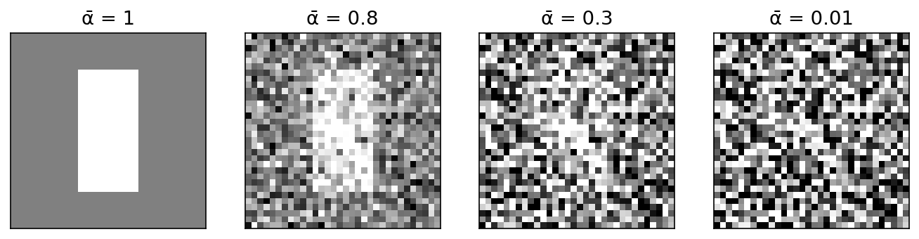
Plain version. The forward process gradually weakens the image signal and adds Gaussian noise. A suitable terminal schedule makes the distribution approximately standard Gaussian.
The idea goes back to Sohl-Dickstein et al. [15], who proposed destroying structure with a slow forward diffusion and learning to reverse it; DDPM [3] made it practical. Let be a data example (an image flattened into numbers, scaled to roughly ). Pick a noise schedule with and write . The forward (noising) process is a Markov chain
where is a Gaussian with mean and covariance , and is the identity. The factor shrinks the signal slightly so that the total variance stays bounded instead of growing; this is why this family is called variance preserving (VP).
Deriving the one-shot formula
Write one step as with . Substituting the previous step,
The two noise terms are independent zero-mean Gaussians, so their sum is Gaussian with variance . Repeating the argument down to gives, with ,
Here is the fraction of signal variance that survives to step , and is a single standard Gaussian vector. This formula is what makes training cheap: we can jump straight to any noise level without simulating the earlier steps.
Noise schedules and the signal-to-noise ratio
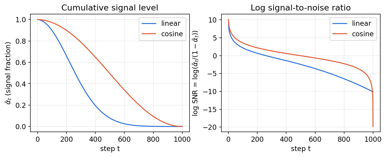
The signal-to-noise ratio at step is
the ratio of signal variance to noise variance (for unit-variance data). It decreases monotonically from very large at to nearly zero at . Two requirements constrain the schedule: must be close to , so that is practically a standard Gaussian (the sampler starts from ); and the steps in between should spend the training budget on noise levels where the network has something useful to learn.
DDPM [3] used and a linear schedule from to . Nichol and Dhariwal [19] observed that this destroys information quickly: for a large part of the chain the image is already nearly pure noise. Their cosine schedule defines with and a small offset , and clips each at . Figure 2 compares the two. Karras et al. [20] later argued that the schedule, the network’s input/output scaling and the distribution of training noise levels are separate design choices that are best tuned independently.
The reverse process and the variational bound
Plain version. To generate, we need the reverse step: “given a noisy example, what did the slightly less noisy example look like?” We cannot compute this directly for real data, but we can compute it if we also know the clean example — and that turns out to give a simple training loss.
The model and the bound
The generative model is a reverse Markov chain that starts at and uses learned Gaussian transitions
where is a neural network (with parameters ) and is a variance we will choose. This is a latent-variable model with latents , exactly like a deep VAE whose encoder is fixed rather than learned (see ML 07). The same Jensen-inequality argument gives an evidence lower bound. Following [3], [15], the negative bound can be rearranged into a sum of KL divergences:
is the Kullback–Leibler divergence. has no learnable parameters (it is small when ); is a decoder term for the last step; and each compares the model’s reverse step with the forward posterior — the reverse step that would be exact if the clean example were known.
The forward posterior is Gaussian
By Bayes’ rule, . Both factors are Gaussian in , so their product is Gaussian. Collecting the quadratic and linear terms in (completing the square) gives
The posterior mean is a weighted average of the clean example and the current noisy one; the posterior variance is slightly smaller than . You do not have to trust the algebra: the snippet below samples the forward chain and fits a regression of on .
Code · Python · 23 lines
import numpy as np

rng = np.random.default_rng(0)
beta = np.linspace(1e-4, 0.02, 1000)
alpha = 1 - beta
abar = np.cumprod(alpha)
t, x0, n = 300, 1.3, 400_000           # check q(x_{t-1} | x_t, x_0) at step t

# Sample the forward chain: x_{t-1} from q(x_{t-1}|x_0), then one more step.
x_prev = np.sqrt(abar[t-1])*x0 + np.sqrt(1-abar[t-1])*rng.normal(size=n)
x_t = np.sqrt(alpha[t])*x_prev + np.sqrt(beta[t])*rng.normal(size=n)

# Empirical regression of x_{t-1} on x_t (the posterior mean is linear in x_t).
slope, intercept = np.polyfit(x_t, x_prev, 1)
resid_var = np.var(x_prev - (slope*x_t + intercept))

# Closed-form posterior from the derivation.
c_x0 = np.sqrt(abar[t-1])*beta[t] / (1-abar[t])
c_xt = np.sqrt(alpha[t])*(1-abar[t-1]) / (1-abar[t])
var = beta[t]*(1-abar[t-1]) / (1-abar[t])
print(f"slope     {slope:.4f}  vs  {c_xt:.4f}")
print(f"intercept {intercept:.4f}  vs  {c_x0*x0:.4f}")
print(f"variance  {resid_var:.6f}  vs  {var:.6f}")
The output matches to three or four decimals (slope 0.9934 vs 0.9930, variance 0.006050 vs 0.006052); the small gaps are Monte Carlo error.
From the bound to the simplified loss
Now use the forward formula backwards: . Substituting into and simplifying with ,
At sampling time the network sees but not . So DDPM parameterizes the model mean in exactly the same form, with the unknown noise replaced by a prediction :
The KL between two Gaussians with the same fixed covariance is a scaled squared distance between their means, so
where does not depend on . Every term of the bound is therefore a weighted noise-prediction error. Ho et al. [3] found that dropping the weight, and sampling uniformly, trains better:
Read it as an algorithm: pick a training example, pick a random step, pick random noise, build in one line, and regress the noise. The time is fed to the network (usually through a sinusoidal embedding) because the same pixel values mean different things at different noise levels.
Two points are easy to get wrong. First, is not the likelihood bound: removing the weights relatively down-weights the low-noise steps, which helps sample quality but hurts the reported log-likelihood. Improved DDPM [19] recovered good likelihoods by learning the variances (as an interpolation between and ) with a hybrid loss. Second, the same network also yields a clean estimate,
which every modern sampler uses internally. When is tiny, the division amplifies prediction errors, so at very high noise is a blurry average, not a sample.
Optional: DDPM (in the Paper guides). Read the original figure, evidence, design choices and limitations.
Noise, clean data, velocity and the score
Plain version. Predicting the noise, predicting the clean image and predicting “which direction makes this example more typical” are three ways to express the same knowledge. They differ in scaling, and scaling changes how the training loss weights different noise levels.
Three parameterizations
Because is a fixed linear relation, a network can output any one of
- the noise (DDPM [3]),
- the clean example ,
- the velocity , introduced by Salimans and Ho [22] for distillation, which stays well scaled at both ends of the schedule.
Given and , each converts to the others exactly. However, an unweighted MSE on , on or on weights the noise levels differently, so the choice affects training. Karras et al. [20] made this explicit with input/output “preconditioning” coefficients that keep the network’s inputs and targets at unit variance for every noise level. Note that this diffusion “velocity” is a reparameterization of signal and noise; it is related to, but not identical with, the transport velocity of flow matching later in this chapter.
Exact conversion does not make finite networks equivalent
For the variance-preserving path, write and . Thus and . The diffusion velocity completes a rotation:
Here are known schedule coefficients; is the target used in [22]; hats denote estimates; and superscripts identify the network’s direct output. The last two conversions require nonzero divisors. Their instability near an endpoint is a numerical and statistical issue, even though the algebra is exact in the interior.
A noise error becomes a clean-image error . Therefore, for corresponding predictions at a fixed noise level,
is the signal-to-noise ratio; the second identity follows from the rotation above. Equal unweighted losses consequently emphasize different times. Changing the target without recording time sampling and loss weighting confounds an experiment [20], [22].
There is also a capacity issue. If a network directly outputs a clean image, its final representation can discard nuisance noise. A network directly outputting noise may need to preserve more coordinates of the noisy input, or use a skip connection that supplies those coordinates. Converting one network’s output afterward does not make its architecture identical to a network trained to output another target. This distinction becomes especially relevant for large pixel patches and high-dimensional latents; the JiT discussion below supplies recent evidence [42]. It does not imply that noise prediction generally fails: the earlier DDPM examples and dense image denoisers are counterexamples.
Code · Python · 28 lines
import numpy as np

rng = np.random.default_rng(7)
x0 = rng.normal(size=32)
eps = rng.normal(size=32)
a, b = np.sqrt(.2), np.sqrt(.8)
xt = a*x0 + b*eps
v_vp = a*eps - b*x0
assert np.allclose(a*xt - b*v_vp, x0)
assert np.allclose(b*xt + a*v_vp, eps)

# A deliberately imperfect noise estimate: compare equivalent losses.
eps_hat = eps + .03*rng.normal(size=32)
x_hat = (xt - b*eps_hat)/a
noise_mse = np.mean((eps_hat - eps)**2)
clean_mse = np.mean((x_hat - x0)**2)
assert np.allclose(clean_mse/noise_mse, b*b/(a*a))
print("Clean/noise MSE ratio:", round(clean_mse/noise_mse, 3))

# A straight flow uses a different path and a different velocity.
t = .35
zt = (1-t)*eps + t*x0
u = x0 - eps
x_from_flow = zt + (1-t)*u
u_from_clean = (x0 - zt)/(1-t)
assert np.allclose(x_from_flow, x0)
assert np.allclose(u_from_clean, u)
print("VP velocity equals straight-flow target:", np.allclose(v_vp, u))
The example prints a loss ratio of 4.0 and False for the two velocity targets. Both use the letter in parts of the literature; a checkpoint’s scheduler must identify the actual path, normalization and time direction.
What is a score, and why does denoising estimate it?
The score of a density is : a vector field that points toward higher probability. If you know the score, you can sample with Langevin dynamics: repeatedly step a little along the score and add a little noise. Song and Ermon [17] trained “noise-conditional score networks” at many noise levels and sampled with annealed Langevin dynamics — a parallel route to diffusion that turned out to be the same idea.
The bridge is denoising score matching (Vincent [16]). For Gaussian corruption, the best possible noise predictor (in mean squared error) is a conditional expectation, , and Tweedie’s formula [40] links it to the score of the noisy marginal :
with the learned score. The same formula in “clean” units reads . Two warnings: this is the score of the noisy marginal distribution at level , not the gradient for any single training image; and it holds for the optimal predictor — a trained network approximates it.
You can verify Tweedie’s formula where everything is known: one-dimensional Gaussian data, for which the best noise predictor is linear in .
Code · Python · 16 lines
import numpy as np

rng = np.random.default_rng(0)
s, abar, n = 0.7, 0.4, 500_000     # data x0 ~ N(0, s^2); one noise level
x0 = s*rng.normal(size=n)
eps = rng.normal(size=n)
xt = np.sqrt(abar)*x0 + np.sqrt(1-abar)*eps

# "Train" the best linear noise predictor eps_hat = w * x_t by least squares.
w = (xt @ eps) / (xt @ xt)
score_from_eps = -w / np.sqrt(1-abar)       # s(x_t) = -eps_hat / sqrt(1-abar)

# Exact: x_t ~ N(0, abar s^2 + 1 - abar), so grad log p_t(x) = -x / var.
exact = -1 / (abar*s**2 + 1 - abar)
print(f"score slope from noise predictor: {score_from_eps:.4f}")
print(f"exact score slope:                {exact:.4f}")
It prints versus : a regression on noise recovers the score.
The SDE view
Song et al. [4] took the step count to infinity. With continuous time and a rate , the VP forward process becomes the stochastic differential equation (SDE)
where is a standard Wiener process (Brownian motion). A classical result says that this process run backwards in time is again an SDE, and that the only unknown in it is the score:
with negative and a reverse-time Wiener process. Moreover, there is a deterministic probability-flow ODE whose solutions have the same marginal distributions at every time:
This unifies the field. DDPM’s ancestral sampler relates to a discretization of the reverse SDE; NCSN [17] corresponds to a “variance exploding” SDE. The probability-flow ODE defines a continuous normalizing flow whose log-density follows an instantaneous change-of-variables identity [4]. The identity is exact; a computed likelihood still has ODE integration error and, when the divergence is estimated stochastically, estimator error. With an approximate learned score, the ODE and reverse SDE need not have identical marginals. The ODE perspective also motivates deterministic sampling and general-purpose numerical solvers.
Sampling is a reverse process
Plain version. A loss evaluated at one random noise level is not a generator. To generate, you must chain many reverse steps with a consistent schedule, starting from pure noise — and you can choose how many steps and how much fresh randomness to inject.
DDPM ancestral sampling
DDPM samples by following the learned reverse chain:
with no noise added at the final step. Ho et al. [3] report similar results for and ; learned variances [19] help most when using fewer steps.
Code: DDPM on a two-dimensional distribution
This complete CPU example (about 10 seconds) uses two Gaussian clusters centered at with standard deviation . It contains every operation of an image model — schedule, random-time training, noise prediction, reverse mean — without an image-scale budget. With 100 steps and this schedule, almost no signal survives to .
Code · Python · 41 lines
import torch
from torch import nn
from torch.nn import functional as F

torch.manual_seed(0)
torch.set_num_threads(1)
T = 100
beta = torch.linspace(.001, .15, T)
alpha = 1-beta
abar = alpha.cumprod(0)
previous = torch.cat([torch.ones(1), abar[:-1]])
post_var = beta * (1-previous) / (1-abar)
net = nn.Sequential(nn.Linear(3, 64), nn.SiLU(),
                    nn.Linear(64, 64), nn.SiLU(), nn.Linear(64, 2))
opt = torch.optim.Adam(net.parameters(), lr=.002)
def data(n):
    side = torch.randint(2, (n, 1))*2-1
    return torch.cat([side*1.5, torch.zeros(n, 1)], 1) + .25*torch.randn(n, 2)
for step in range(3000):
    x0 = data(128)
    t = torch.randint(T, (len(x0),))
    eps = torch.randn_like(x0)
    a = abar[t, None]
    xt = a.sqrt()*x0 + (1-a).sqrt()*eps
    predicted = net(torch.cat([xt, t[:, None].float()/(T-1)], 1))
    loss = F.mse_loss(predicted, eps)
    opt.zero_grad(); loss.backward(); opt.step()
net.eval()
with torch.no_grad():
    x = torch.randn(512, 2)
    for t in reversed(range(T)):
        time = torch.full((len(x), 1), t/(T-1))
        eps = net(torch.cat([x, time], 1))
        mean = (x-beta[t]/(1-abar[t]).sqrt()*eps)/alpha[t].sqrt()
        x = mean + post_var[t].sqrt()*torch.randn_like(x) if t else mean
    assert torch.isfinite(x).all()
    print("terminal signal:", round(abar[-1].item(), 6))
    left = x[x[:, 0] < 0]
    print("fraction in left cluster:", round((x[:, 0] < 0).float().mean().item(), 3))
    print("left cluster: mean x", round(left[:, 0].mean().item(), 2),
          "std", round(left[:, 0].std().item(), 2), "(data: -1.5 and 0.25)")
On our machine it prints a terminal signal of 0.000349, a left-cluster fraction of 0.441, and a left-cluster mean and standard deviation of and . The cluster shapes are right; the 44/56 split shows the small network has not learned the mode weights exactly. This is why a single summary number is never enough: always plot samples, and check mode coverage, within-mode spread and outliers against fresh data.
DDIM: same training, different sampler
Song, Meng and Ermon [5] noticed that only depends on the marginals , not on the Markov chain that produced them. Many non-Markovian forward processes share those marginals, and each gives a different reverse sampler — all usable with the same trained . The DDIM update, for any decreasing subsequence of steps , is
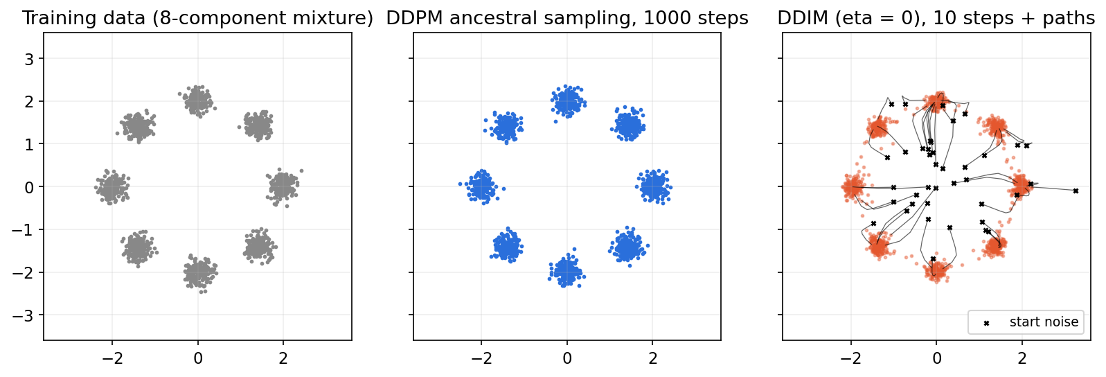
where is the clean estimate at and controls stochasticity. Read it as: “estimate the clean example, then re-noise it to the next, lower noise level using the predicted noise direction.” With and consecutive steps, this recovers DDPM’s posterior variance; with the sampler is deterministic and is a discretization of the probability-flow ODE. Determinism has practical consequences: the same starting noise always gives the same output, so you can interpolate in noise space or invert a real image to its noise (DDIM inversion), which is the basis of many editing methods.
The following standalone example repeats the same small training setup so it can run independently. When experimenting in one session, reuse the already trained net, abar and T instead:
Code · Python · 50 lines
import torch
from torch import nn
from torch.nn import functional as F

torch.manual_seed(0)
torch.set_num_threads(1)
T = 100
beta = torch.linspace(.001, .15, T)
alpha = 1-beta
abar = alpha.cumprod(0)
previous = torch.cat([torch.ones(1), abar[:-1]])
post_var = beta * (1-previous) / (1-abar)
net = nn.Sequential(nn.Linear(3, 64), nn.SiLU(),
                    nn.Linear(64, 64), nn.SiLU(), nn.Linear(64, 2))
opt = torch.optim.Adam(net.parameters(), lr=.002)
def data(n):
    side = torch.randint(2, (n, 1))*2-1
    return torch.cat([side*1.5, torch.zeros(n, 1)], 1) + .25*torch.randn(n, 2)
for step in range(3000):
    x0 = data(128)
    t = torch.randint(T, (len(x0),))
    eps = torch.randn_like(x0)
    a = abar[t, None]
    xt = a.sqrt()*x0 + (1-a).sqrt()*eps
    predicted = net(torch.cat([xt, t[:, None].float()/(T-1)], 1))
    loss = F.mse_loss(predicted, eps)
    opt.zero_grad(); loss.backward(); opt.step()
net.eval()

def ddim_sample(n, steps, eta=0.0, seed=1):
    g = torch.Generator().manual_seed(seed)
    taus = torch.linspace(T-1, 0, steps).round().long()
    x = torch.randn(n, 2, generator=g)
    with torch.no_grad():
        for i, t in enumerate(taus):
            time = torch.full((n, 1), t.item()/(T-1))
            eps = net(torch.cat([x, time], 1))
            a_t = abar[t]
            a_prev = abar[taus[i+1]] if i+1 < steps else torch.tensor(1.)
            x0_hat = (x - (1-a_t).sqrt()*eps) / a_t.sqrt()
            sigma = eta*((1-a_prev)/(1-a_t)*(1-a_t/a_prev)).sqrt()
            x = (a_prev.sqrt()*x0_hat + (1-a_prev-sigma**2).sqrt()*eps
                 + sigma*torch.randn(n, 2, generator=g))
    return x

for steps in [5, 20, 100]:
    s = ddim_sample(2000, steps)
    left = s[s[:, 0] < 0]
    print(f"{steps:3d} steps: left fraction {(s[:, 0] < 0).float().mean():.3f}, "
          f"left-cluster mean x {left[:, 0].mean():.2f}, std {left[:, 0].std():.2f}")
The output shows the typical pattern. With 5 steps the left cluster is centered at with standard deviation — the samples are pulled toward the middle and smeared, because large steps follow a curved trajectory with straight lines. With 20 steps it is and ; with 100 steps and , close to the data. No retraining was needed to change the step count.
Faster solvers
Once sampling is “solve an ODE,” numerical analysis applies. Karras et al. (EDM) [20] used a second-order Heun solver with a carefully chosen spacing of noise levels and showed that sampler, schedule, preconditioning and training noise distribution can be tuned separately. DPM-Solver [21] exploits the semi-linear structure of the diffusion ODE — the linear part can be integrated exactly — to reach good quality in around 10 network evaluations. Stochastic samplers add a little fresh noise at each step; that costs more steps but can correct accumulated errors. Whatever the solver, report the number of function evaluations (NFE): the number of network calls, which, rather than “steps,” is the true sampling cost.
Steering generation: conditioning and guidance
Plain version. Conditioning specifies the requested output; guidance adjusts how strongly sampling favors it. More guidance need not mean a better image.
Conditioning
A conditional model learns for a condition . Class labels enter through embeddings added to the time embedding; text enters through cross-attention from image features to text-encoder tokens [7]; images (for super-resolution, inpainting, editing) are concatenated to the input channels or fed through extra encoders.
Classifier guidance
Bayes’ rule for the noisy marginals gives . Dhariwal and Nichol [18] trained a separate classifier on noisy images and added its gradient, scaled by , to an unconditional model. In noise units,
A scale samples roughly from , a sharpened distribution that trades diversity for fidelity. Together with architecture improvements, this was the work that showed diffusion models beating GANs on ImageNet [35] sample quality [18]. Its drawback is the extra classifier, which must be trained on noisy inputs for every noise level.
Classifier-free guidance (CFG)
Ho and Salimans [6] removed the classifier. During training, the condition is replaced by a “null” token for a random fraction of examples, so one network learns both and . Bayes’ rule says the classifier gradient equals the difference of the conditional and unconditional scores, so the implicit-classifier version of the formula above is
In this convention is unconditional, is the ordinary conditional model, and extrapolates past it. (Some papers write the same thing as , so their “scale” is in our notation; always check the convention before comparing numbers.)
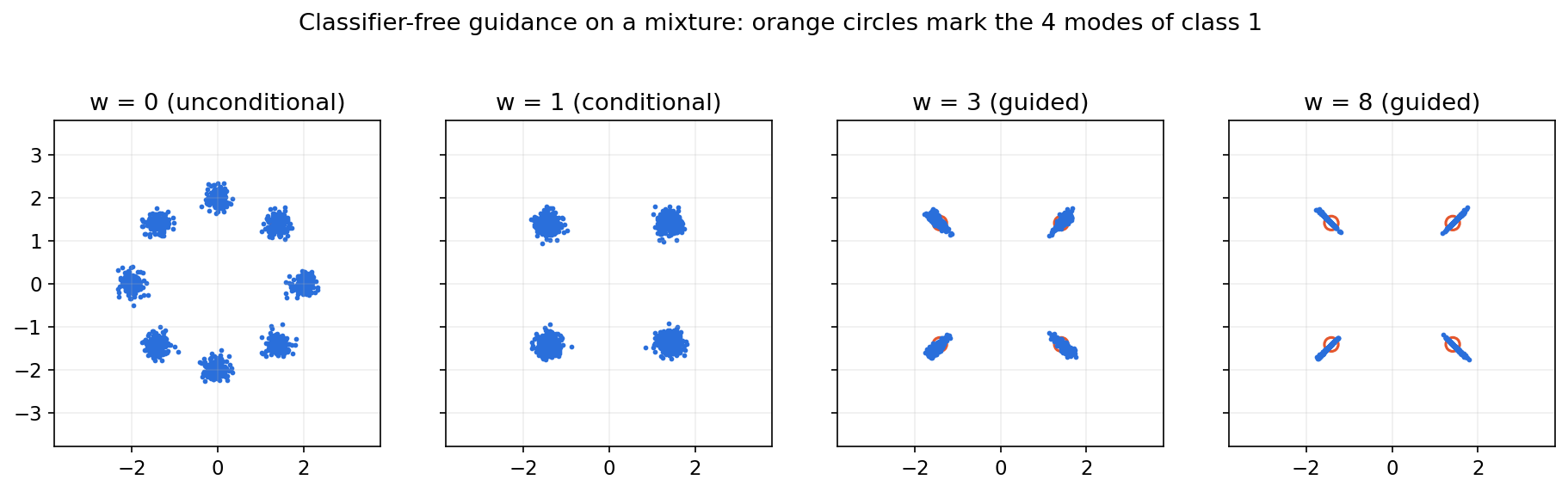
The snippet below uses the exact noise predictor of a four-blob mixture, so any odd behaviour is due to guidance itself, not to a badly trained network. Class 1 is the two blobs with .
Code · Python · 32 lines
import numpy as np

# Data: four Gaussian blobs at the corners of a square; class c is the sign of x.
MU = np.array([[-1.5, -1.5], [-1.5, 1.5], [1.5, -1.5], [1.5, 1.5]])
SIG = 0.2
CLASS = np.array([0, 0, 1, 1])

def eps_exact(x, abar, comps):
    """Exact E[eps | x_t] for a Gaussian mixture restricted to `comps`."""
    m = np.sqrt(abar)*MU[comps]
    var = abar*SIG**2 + 1 - abar
    logw = -((x[:, None] - m[None])**2).sum(-1) / (2*var)
    w = np.exp(logw - logw.max(1, keepdims=True))
    w /= w.sum(1, keepdims=True)
    score = -(w[..., None]*(x[:, None] - m[None])).sum(1) / var
    return -np.sqrt(1-abar)*score

abar = np.cumprod(1 - np.linspace(1e-4, 0.02, 1000))
taus = np.linspace(999, 0, 50).round().astype(int)
everything, class1 = np.arange(4), np.where(CLASS == 1)[0]
print("data: mean distance to its mode", round(SIG*np.sqrt(np.pi/2), 3))
for w in [0, 1, 3, 8]:
    x = np.random.default_rng(0).normal(size=(4000, 2))
    for i, t in enumerate(taus):                    # deterministic DDIM
        e_u, e_c = eps_exact(x, abar[t], everything), eps_exact(x, abar[t], class1)
        e = e_u + w*(e_c - e_u)                     # classifier-free guidance
        x0 = (x - np.sqrt(1-abar[t])*e) / np.sqrt(abar[t])
        a_prev = abar[taus[i+1]] if i+1 < len(taus) else 1.0
        x = np.sqrt(a_prev)*x0 + np.sqrt(1-a_prev)*e
    dist = np.linalg.norm(x[:, None] - MU[None], axis=-1).min(1)
    print(f"w={w}: class-1 fraction {(x[:, 0] > 0).mean():.3f}, "
          f"mean distance to nearest mode {dist.mean():.3f}")
The data’s mean distance to its mode is 0.251. With about half the samples (0.490) are class 1; with all of them are, at distance 0.225 (50 DDIM steps slightly under-disperse). At the distance is 0.259 and at it grows to 0.446: strong guidance does not just “make it more class 1” — it pushes samples past the data, a toy version of the over-saturated colours and distorted shapes seen with very high guidance in image models. Figure 4 shows the same effect on the 8-mode mixture.
Guidance has a compute cost too: each step needs a conditional and an unconditional prediction, so a 30-step guided sampler costs 60 network evaluations unless the two are fused. And is a sampling knob, not a calibrated measure of how well the image matches the prompt.
Latent diffusion and diffusion transformers
Plain version. Pixels are expensive. Compress the image into a smaller grid of features with an autoencoder, run diffusion in that compressed space, then decode. Separately, the denoising network itself can be a transformer instead of a convolutional U-Net [37].
Latent diffusion
Rombach et al. [7] train an autoencoder first: an encoder maps an image to an latent with a spatial downsampling factor , and a decoder maps back. The autoencoder is trained with reconstruction, perceptual and adversarial losses plus a light regularizer (a small KL term toward a Gaussian, or vector quantization) so that the latent space stays well behaved. Diffusion is then trained on exactly as before, and generation ends with . With , a image becomes a latent: 64 times fewer spatial positions for every network call.
The trade-off is a reconstruction bottleneck: information discarded by the encoder cannot be faithfully recovered from that code, although the decoder may synthesize plausible detail. The latent’s scale must also match what the diffusion model was trained on; implementations rescale latents to roughly unit variance. Text conditioning in [7] uses cross-attention layers in the U-Net, the design behind the Stable Diffusion family.
Diffusion transformers
DiT (Peebles and Xie [8]) replaces the U-Net with a Vision Transformer [41] (see ML 05) over latent patches. A latent of size is cut into patches, giving tokens; smaller means more tokens, more compute and better quality. The timestep and class label condition every block through adaptive layer norm: they predict the scale and shift of each LayerNorm, and in the “adaLN-Zero” variant also a gating factor initialized to zero, so each residual block starts as the identity. The paper’s main finding is a scaling trend: across model sizes and patch sizes, more transformer compute (GFLOPs) gave consistently lower FID [8].
It helps to keep three choices separate. The architecture (U-Net or transformer) is the function approximator. The objective (noise, , , or flow velocity) is what it regresses. The sampler (DDPM, DDIM, ODE solver) is how predictions become an image. Stable Diffusion 3 [9] is an example of a new combination: a latent transformer with separate weights for the image and text token streams that attend jointly (“MM-DiT”), trained with a rectified-flow objective and a timestep distribution biased toward intermediate noise levels.
For video, the latent and the attention must cover time as well as space, so compression and attention patterns become the main engineering problem. Melnik et al.’s survey [31] reviews architectures, temporal-consistency mechanisms and evaluation for video diffusion. Per-frame quality is not enough there: object permanence, motion plausibility and long-duration consistency need their own evaluation.
Pixel space, latent space and representation autoencoders
Plain version. The generator needs a place to do its repeated updates. That place can be the image itself, a compact reconstruction code, or features learned by a visual representation model. A latent stage buys a particular computational and statistical trade-off; it is not a prerequisite for generative modeling.
Why pixels become latents and then pixels again
Training images arrive as pixels, while the output must be viewable as pixels. Between these endpoints, an encoder can remove redundancy and produce a grid that is cheaper to update repeatedly [7]. Train the encoder and decoder on reconstruction first, then fit a generative distribution to encoded training images. These are two different tasks: reconstruction preserves a given example; generation learns which encoded examples are plausible.
The training and sampling routes are
Here is a training image; and are the encoder and decoder; is an encoded image; is its corrupted state; parameterizes the generative predictor; is a generated code; is the generated image; and is a reconstruction. Pure text-to-image sampling does not encode an input image first. Editing and image-to-image generation can encode an actual input image and begin from a partially corrupted code.
The main saving occurs because the denoiser or flow predictor runs repeatedly, while encoding training data and decoding a sample occur much less often. A spatial factor reduces grid positions by , but the number of latent channels also matters. For an image with three channels and a latent with channels, the scalar-count reduction is . It is incorrect to describe the grid reduction as the reduction in all floating-point values or total runtime.
For a transformer, token count and token width must also be distinguished. Full attention stores a matrix with a number of entries proportional to , where is the token count; feature projections depend on token width as well [41]. A patch size can reduce in either pixels or latents. None of these counts alone predicts wall-clock speed because kernels, memory traffic, the decoder and conditioning contribute.
Code · Python · 15 lines
# Synthetic shape bookkeeping, not a benchmark or a specific checkpoint.
H = W = 512
channels, spatial_factor, patch = 4, 8, 2
pixel_values = H*W*3
h = H//spatial_factor
w = W//spatial_factor
latent_values = h*w*channels
pixel_tokens = (H//patch)*(W//patch)
latent_tokens = (h//patch)*(w//patch)
print("Spatial positions reduction:", (H*W)//(h*w))
print("Scalar values reduction:", pixel_values//latent_values)
print("Dense attention entries reduction:", pixel_tokens**2//latent_tokens**2)
assert pixel_values//latent_values == 48
assert pixel_tokens//latent_tokens == 64
assert pixel_tokens**2//latent_tokens**2 == 4096
This constructed example yields 64 times fewer spatial positions, 48 times fewer scalar values and 4096 times fewer attention entries at the same numerical patch size in each coordinate space. Changing patch sizes changes the comparison. A pixel transformer with much larger patches can have the same token count as a latent transformer.
The cost is information loss. If two images have the same code, a deterministic decoder cannot recover their different exact details. A decoder may invent plausible texture, but that does not restore information about the original image. The reconstruction check therefore deserves its own evaluation before generative training. Inspect fine lines, lettering and temporal changes, rather than relying only on average image error.
The following deliberately simple encoder averages blocks and the decoder repeats those averages. It demonstrates a bottleneck without pretending to reproduce a learned VAE or RAE.
Code · Python · 13 lines
import numpy as np

y, x = np.mgrid[:64, :64]
checker = ((x+y) % 2).astype(float)
smooth = x/63
image = .6*smooth + .4*checker
f = 4
latent = image.reshape(64//f, f, 64//f, f).mean(axis=(1, 3))
reconstruction = np.repeat(np.repeat(latent, f, axis=0), f, axis=1)
print("Synthetic reconstruction MSE:", round(np.mean((image-reconstruction)**2), 6))
assert np.mean((image-reconstruction)**2) > .04
# Recovering the exact latent does not recover the missing checkerboard.
assert np.allclose(reconstruction[0, :f], reconstruction[0, 0])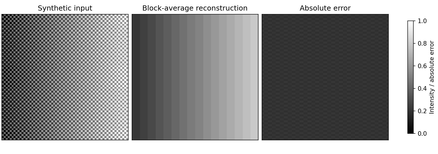
For editing, repeatedly encoding and decoding a result can accumulate distortion. Keep intermediate edits in the compatible latent space when the pipeline permits it, and inspect the eventual pixel output. A good unconditional generator may still be a poor reconstruction system. The claim that an autoencoder sets a ceiling concerns faithfulness to encoded information; it does not mean that a generative decoder can never synthesize new fine texture.
Reconstruction codes versus semantic representation codes
A VAE encoder is trained with a reconstruction objective and a distributional regularizer; its code is designed to support decoding and sampling [7]. A pretrained recognition encoder instead learns useful visual features. These goals can align, but recognition invariance may discard details needed for faithful reconstruction. The decoder and the retained feature structure determine whether the representation is a useful generative space.
Zheng, Ma, Tong and Xie’s Representation Autoencoders (RAEs) [43] pair a frozen pretrained representation encoder with a trained decoder. Their ICLR 2026 study uses semantic visual features as the space for generative modeling. It examines high-dimensional token features, dimension-dependent noise scheduling, decoder robustness and a shallow wide diffusion head. This changes the representation being generated, rather than simply adding a feature-alignment loss to a conventional latent predictor.
Do not equate “latent” with “smaller in every dimension.” A spatially sparse feature grid can have many channels per token. An RAE is also not automatically a variational model: a frozen feature extractor plus a decoder does not by itself define a Gaussian posterior, a KL regularizer or a likelihood bound. Keep reconstruction, representation quality and generative quality as separate measurements.
Tong et al. [44] extend this approach to freeform text-to-image generation in 2026. Their study compares RAE and VAE spaces at larger scales and examines decoder data composition. It finds that dimension-aware noise scheduling remains important while some small-scale architectural and decoder modifications offer little benefit at the tested larger scales. This is a reason to re-test recipes when scale and data change, rather than treating an ImageNet result as a universal design rule.
For a new application, inspect whether the chosen encoder preserves the content that matters: fine text for documents, small defects for inspection, or frame-to-frame differences for video. Evaluate the decoder on held-out real features and on generated features. A decoder trained only on exact training codes can be sensitive to small off-distribution errors in a sampled code. Normalize features using the training recipe, and record the encoder version with the generative checkpoint.
JiT: direct clean-image prediction on pixels
Li and He’s Just image Transformers (JiT) [42], published at CVPR 2026 after a 2025 preprint, revisit large-patch transformers operating directly on pixels. The network predicts the clean image; sampling derives a flow velocity from that prediction. Their controlled experiments support a manifold-based explanation: a bottleneck can retain structured clean-image information while making direct prediction of high-dimensional noise or velocity difficult. The reported setup uses no pretrained latent tokenizer or auxiliary representation loss. This is evidence for a particular architecture and training regime, not a proof that pixel-space models always outperform latent generators.
The crucial distinction is direct network output versus the quantity used in the loss or solver. For the straight path defined below, use , with noise at and clean data at . A network that directly predicts can supply
Here is the clean image; is the noise draw; is their interpolation; is the direct prediction; and is the corresponding transport velocity. The identity holds for before numerical clipping. An -output network can thus train with a velocity-space loss. Calling it “clean prediction” does not mean its loss is an unweighted clean-image MSE. JiT’s released implementation makes this distinction explicit [42].
Near , division by needs an endpoint convention and numerical safeguards. For the interior algebra, a fixed clean-image error is amplified increasingly as the endpoint approaches. During sampling, use the checkpoint’s time distribution, noise scaling and solver recipe. Changing the direct output label alone does not reproduce the method.
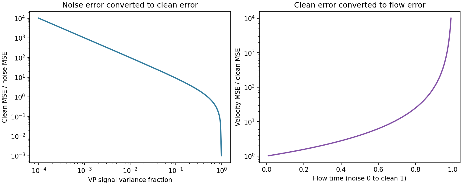
A useful comparison fixes training data, compute, resolution, token count and the sampler, then changes the representation or target one at a time. Compare a pixel transformer, a compact VAE-latent transformer and a representation-latent transformer on reconstruction needs, generated quality and total cost. Record encoder/decoder cost and any representation pretraining. A model that uses a pretrained visual encoder has inherited training even when its generative stage starts from scratch.
Optional: JiT (in the Paper guides). Inspect the pixel architecture and the prediction-space ablation.
Flow matching: learn a transport velocity
Plain version. For a straight conditional path, pair noise with data and regress its velocity. Generation follows the learned velocity field, whose trajectories need not be straight.
Time convention change. In this section time runs from noise at to data at , the opposite of the diffusion sections above (where large meant more noise).
The conditional flow-matching objective
A continuous normalizing flow moves points with an ODE . If the velocity field is right, it transports the noise distribution to the data distribution . Lipman et al. [10] (and, concurrently, Liu et al. [11] and Albergo and Vanden-Eijnden’s stochastic interpolants [34]) showed how to train without ever simulating the ODE.
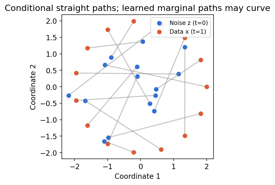
Pair noise with a data example and define the straight conditional path
Every pair moves at constant speed in a straight line. The marginal velocity we actually want is the average of these conditional velocities over all pairs that pass through the point:
We cannot compute this average, but we do not need to. Compare the “ideal” loss with the one we can compute:
with . Expand both squares. The terms are identical. The cross terms are equal because, by the tower rule, . The remaining terms do not involve . Therefore
so regressing the per-pair velocity trains the marginal velocity field. This is the same trick as in diffusion: a target that is noisy for any single example has the right conditional mean. Generation solves from to with any ODE solver.
How flow matching relates to diffusion
The linear path is a Gaussian path: given , . Writing (a noise prediction) and using ,
So a flow-matching velocity, a noise predictor and a score are again interchangeable for this path; what differs is the path (straight lines versus the VP curve), the weighting of noise levels in the loss, and the time convention. Diffusion’s probability-flow ODE is itself a flow along a particular Gaussian path. Lipman et al.’s guide [2] and the stochastic-interpolant framework [34] treat both as special cases of one construction. The practical advice is the same as for parameterizations: the targets are related by derivation, not interchangeable by renaming.
Code: flow matching on two clusters
This standalone example learns the same two-cluster distribution as the DDPM snippet with linear conditional paths, then samples with Euler steps of size .
Code · Python · 32 lines
import torch
from torch import nn
from torch.nn import functional as F

torch.manual_seed(0)
torch.set_num_threads(1)
net = nn.Sequential(nn.Linear(3, 64), nn.SiLU(),
                    nn.Linear(64, 64), nn.SiLU(), nn.Linear(64, 2))
opt = torch.optim.Adam(net.parameters(), lr=.002)
for step in range(3000):
    z = torch.randn(128, 2)
    side = torch.randint(2, (128, 1))*2-1
    x = torch.cat([1.5*side, torch.zeros(128, 1)], 1) + .25*torch.randn(128, 2)
    t = torch.rand(128, 1)
    xt = (1-t)*z+t*x
    loss = F.mse_loss(net(torch.cat([xt, t], 1)), x-z)
    opt.zero_grad(); loss.backward(); opt.step()
net.eval()
def euler_sample(n, steps, seed=1):
    x = torch.randn(n, 2, generator=torch.Generator().manual_seed(seed))
    with torch.no_grad():
        for k in range(steps):
            t = torch.full((n, 1), k/steps)
            x = x + net(torch.cat([x, t], 1))/steps
    return x

for steps in [1, 4, 50]:
    s = euler_sample(2000, steps)
    assert torch.isfinite(s).all()
    left = s[s[:, 0] < 0]
    print(f"{steps:2d} Euler steps: left fraction {(s[:, 0] < 0).float().mean():.3f}, "
          f"left-cluster mean x {left[:, 0].mean():.2f}, std {left[:, 0].std():.2f}")
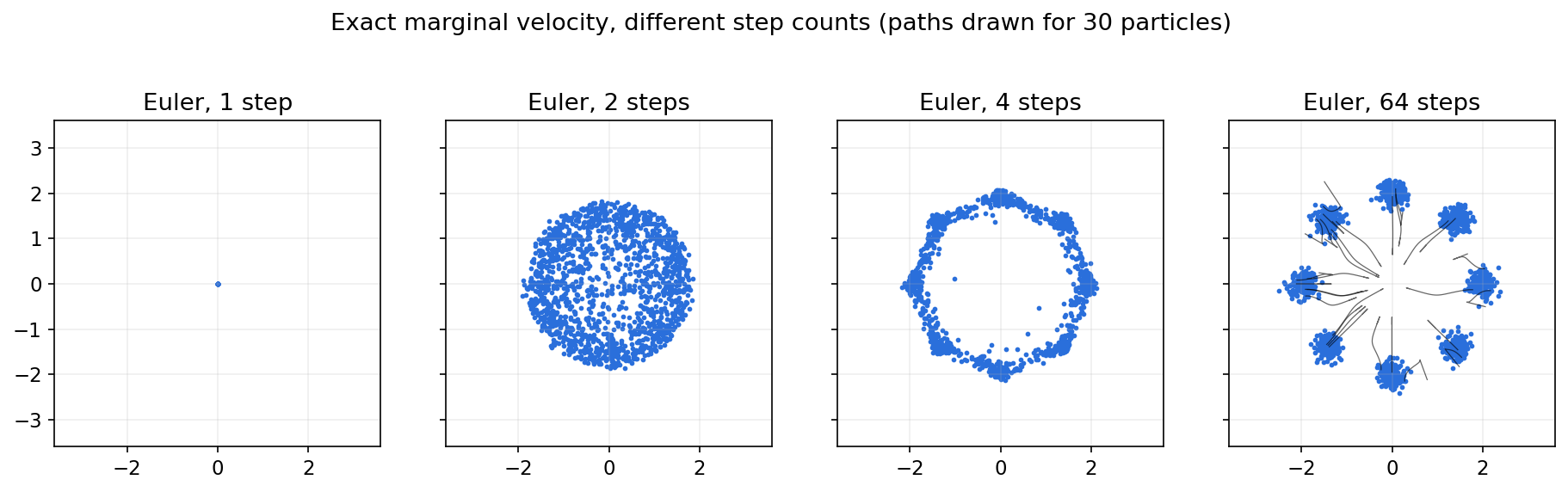
It prints, for 1, 4 and 50 steps, left-cluster means of , and with standard deviations , and . One Euler step lands almost at the overall data mean: at the marginal velocity is , so a single full step sends every noise point to . Straight conditional paths do not make the learned marginal flow straight. Figure 8 shows the same effect with the exact velocity of an 8-mode mixture.
Rectified flow and reflow
Liu, Gong and Liu [11] use the same straight interpolation (“rectified flow”) and add reflow: after training, generate pairs by solving the learned ODE from each , then retrain on these coupled pairs instead of independent ones. Because the new pairs are already connected by the flow, their straight lines cross less, the learned trajectories become straighter, and fewer Euler steps are needed; a straight enough flow can then be distilled into a one-step model. Stable Diffusion 3 [9] showed that rectified-flow training of a large latent transformer works at text-to-image scale.
Optional: Flow Matching (in the Paper guides). Read the original figure, evidence, design choices and limitations.
After flow matching: intervals, image outputs and one-step pixels
Plain version. There are two separate questions after learning a flow: can one prediction cover a whole interval, and what should the network directly output? MeanFlow changes the interval being modeled; JiT changes the output representation. Pixel MeanFlow brings these directions together. Read them in that order instead of treating every new name as another sampler.
First align the clocks
The preceding flow-matching example moves from noise at zero to data at one. MeanFlow [13], improved MeanFlow [49] and pixel MeanFlow [50] use the reverse convention:
Here is a clean training example, is prior noise, and is their interpolated training state. Generation runs from one to zero. To compare with JiT’s time , use and reverse the velocity sign. This is a coordinate change, not a different generative principle. The conditional straight interpolation used to form training pairs still does not imply that the learned marginal ODE trajectories are straight.
MeanFlow: replace a tangent with an interval average
An instantaneous velocity tells you which way to move now. MeanFlow [13] learns the average over an interval, so a prediction can describe its entire displacement:
Here is the marginal instantaneous velocity, lies on its ODE trajectory, are interval endpoints, and is the average velocity along that trajectory. The zero-length boundary uses the limit . This integral defines the desired quantity; training does not obtain a teacher trajectory by evaluating it for every example.
Instead, differentiating the definition yields . The total derivative follows the moving state and holds fixed; it is not merely a partial derivative with respect to the time input. The original recipe uses a Jacobian-vector product and a stopped-gradient target constructed from the current network. One-call generation then uses the full interval , provided the learned average is accurate enough.
The following exact curve illustrates the distinction. It is an algebra check, not a trained MeanFlow model:
Code · Python · 9 lines
r, t = 0.0, 1.0
start = (t, t*t)                    # curve z(t) = (t, t^2)
instant = (1.0, 2*t)                # tangent at the starting time
average = (1.0, t+r)                # exact interval-average derivative
one_euler = tuple(z-(t-r)*v for z, v in zip(start, instant))
one_average = tuple(z-(t-r)*u for z, u in zip(start, average))
assert one_average == (r, r*r)
print("Instantaneous Euler jump:", one_euler)
print("Average-velocity jump:", one_average)
The outputs are (0.0, -1.0) and (0.0, 0.0). A correct local tangent can miss the endpoint after one large step, whereas the correct interval average reaches it. Learning that average is the difficult part.
Optional: MeanFlow (in the Paper guides). Read the original figure, controlled comparisons and limitations.
Improved MeanFlow: make prediction inputs and guidance explicit
iMF [49] rewrites training as a loss on instantaneous velocity while the network still outputs average velocity. The important change is inside the derivative calculation: the original recipe feeds the sampled conditional velocity into the JVP; iMF uses a network prediction of marginal velocity. This keeps the clean training label out of the compound predictor’s inputs. It can reuse the zero-length boundary or use an auxiliary velocity head during training.
A separate improvement makes guidance scale and its active interval explicit conditions. A single trained model can then vary those settings at inference while retaining one-call generation. That is different from adding two conditional/unconditional network calls afterward. Its in-context condition tokens also change model size, so the final system comparison is not a pure loss-function ablation.
Optional: Improved MeanFlow (in the Paper guides). Read the original figure, controlled comparisons and limitations.
JiT: image output is a different design axis
The earlier JiT discussion separates direct clean-image output from velocity-space loss [42]. In the time convention used here, the derived instantaneous velocity is , where is the predicted clean image. This conversion needs care near zero. JiT still follows a multi-step trajectory; an image-shaped output does not automatically provide an interval-average velocity or a one-step sample.
The controlled comparison is especially useful: hold loss space fixed, then change direct output and patch dimension. It explains why algebraic conversions between targets do not make finite-capacity networks equally easy to train. Do not compare only the strongest headline models with different training recipes.
Optional: JiT (in the Paper guides). Read the original figure, controlled comparisons and limitations.
Pixel MeanFlow: connect image output to the interval field
Pixel MeanFlow [50] defines a two-time image-like field . Here is induced by the average-velocity field, not necessarily the clean training image paired with . The network predicts this field as ; converting back gives . This conversion uses with endpoint safeguards.
The derived enters iMF’s instantaneous-velocity loss: image output → average velocity → instantaneous-velocity loss. For the full interval, the update simplifies to the network’s image output, enabling one-call pixel generation. At intermediate intervals, the image-like manifold interpretation is a hypothesis supported by the paper’s visualizations and ablations, not an exact manifold guarantee.
No latent tokenizer is needed at generation, but the stronger recipe uses pretrained feature networks for perceptual training losses. Record that training dependency when comparing it with JiT’s recipe or a latent generator. “No decoder,” “one NFE” and “no pretrained component anywhere” are three different claims.
Optional: Pixel MeanFlow (in the Paper guides). Read the original figure, controlled comparisons and limitations.
Keep neighboring approaches separate
Reflow [11] changes the coupling of training pairs to straighten trajectories. Consistency models [12] learn agreement of endpoint predictions along a trajectory; teacher-based distillation and teacher-free training are separate settings. MeanFlow instead parameterizes an interval average, while JiT addresses the network output space. The few-step overview compares these neighboring families.
Before choosing a method, write down its representation, direct output, loss target, time direction and sampling calls. Then compare matched resolution and conditioning, distinguish generator training from representation pretraining, and include decoder cost where relevant. A lower NFE is useful evidence about calls, not a complete latency or quality evaluation.
Pretrained image and video generators as complete pipelines
Plain version. A pretrained generator is a bundle of compatible components. Loading the denoiser weights alone does not establish the right representation, text conditioning, prediction target or sampling schedule. The image/video boundary also changes what a reconstruction must preserve.
Read the components before running the checkpoint
A practical pipeline combines a text encoder, an optional image/video encoder, a time-conditioned predictor, a sampler and an optional decoder. A separate refinement model may follow the first generator. Each component expects particular tensor shapes and scales. A scheduler declaring v_prediction may mean VP velocity; a flow scheduler may expect a derivative along a straight interpolation. Check the training path rather than guessing from a configuration string.
The following verified examples illustrate architectural differences. They are fixed research baselines, rather than a ranking of the latest product releases. The references include their papers or technical reports and official release documentation.
| Baseline | Generation representation and predictor | What to inspect in the pretrained pipeline |
|---|---|---|
| SDXL [45] | Reconstruction latents with a convolutional denoiser | Text conditioning, latent scaling, optional base/refiner composition and compatible sampling configuration |
| Stable Diffusion 3 [9] | Latent rectified flow with a joint text–image transformer | Flow time convention, text streams, time sampling and autoencoder compatibility |
| FLUX.1 [46] | Latent rectified-flow transformer | Exact release variant, guidance behavior, text conditioning, autoencoder and release terms |
| JiT [42] | Class-conditioned clean-image prediction directly on pixels | Image normalization, patch/resolution configuration, derived velocity and sampling recipe; this is not a freeform text-to-image checkpoint |
| HunyuanVideo [47] | Compressed video latents with a flow-matching transformer | Video autoencoder, image/video joint training, temporal dimensions and text-conditioning components |
| Wan2.1 [48] | Video diffusion transformer with a spatiotemporal autoencoder | Text-to-video versus image-to-video variant, causal video compression, temporal length and decode caching |
SDXL [45] documents a larger latent image-generation architecture and optional refinement stage. Stable Diffusion 3 [9] illustrates how the same broad latent pipeline can instead use rectified flow and joint text/image attention. FLUX.1’s official model card [46] describes a released rectified-flow transformer; its .1-dev variant is guidance-distilled. These facts do not make the checkpoints interchangeable. Ordinary two-pass CFG and a distilled guidance input can have different meanings and costs.
For image-to-image generation, encoding an input and adding partial noise trades input preservation against the ability to change it. The actual noise level is determined by the schedule, not merely by a UI label such as “strength.” To compare edits, keep the same input and record the initial time, seed, prompt, guidance and reconstruction baseline. A reconstruction artifact can otherwise be mistaken for an edit requested by the text.
Video adds temporal compression and a consistency problem
Let a video have frames, height and width . A hypothetical encoder compressing time by and each spatial axis by gives a rough latent grid of positions. Exact shapes depend on padding and special handling of the first frame. After patching, dense attention across all positions grows quadratically with the remaining token count; separately reducing time and space can therefore change cost substantially.
HunyuanVideo’s technical report [47] combines a 3D video autoencoder with a flow-matching transformer and staged image/video training. Wan’s report [48] explains a causal video VAE with special first-frame handling, spatial and temporal compression, and feature caching during chunked encoding/decoding. Causality in an autoencoder does not by itself imply that the entire video generator samples autoregressively; the generative attention and sampling procedure must be examined separately.
A frame can look excellent while a clip changes an object’s identity, reverses motion unexpectedly or forgets an occluded object. Test reconstruction of held-out clips before generation, then evaluate appearance, motion, prompt correspondence and consistency across frames. Melnik et al. [31] provide the survey map for these video-specific issues. A per-image metric alone cannot diagnose temporal behavior.
A pretrained video generator also does not automatically become a reliable world model. Predicting plausible clips differs from predicting the consequences of a specified action. The world-model chapter develops this distinction through state, actions, rollouts and evaluation. Use the actual conditioning interface and evaluate the task the system claims to solve.
A reproducible first experiment
Start by recording a pipeline manifest: checkpoint revision, encoder/decoder revisions, text encoder, representation shape and scaling, prediction target, time direction, solver, evaluation count, guidance, dtype and seed. Then perform a reconstruction check if an autoencoder is present and generate a fixed small prompt/seed set. Compare one change at a time. Include decoder latency and peak memory when reporting the cost of a latent method.
This chapter’s CPU examples test the underlying identities and failure modes without downloading weights. Full-resolution pretrained generation belongs in a separately provisioned experiment using the official release instructions [42], [45]–[48]. Treat an actual measured run, a paper’s published result and a toy calculation as three different kinds of evidence.
Few-step and one-step generation
Plain version. If a sampler needs 50 network calls, train a second model that jumps along the trajectory in a few calls — or train one from scratch that is designed to jump.
The main families are:
- Progressive distillation [22]: a student learns to match two deterministic teacher steps with one step; repeating the procedure halves the step count each round.
- Consistency models [12]: learn a function that maps any point on a probability-flow ODE trajectory to that trajectory’s starting (clean) point. It must satisfy the boundary condition at the smallest time , enforced by writing with and . Training asks outputs at adjacent points of a trajectory to agree. In consistency distillation, adjacent points come from one ODE-solver step of a pretrained diffusion model; in consistency training, from the same data example noised at two levels, with no teacher. Sampling takes one step, or a few steps of “jump to clean, re-noise, jump again.” Improved training recipes [32] simplified continuous-time consistency models and scaled them to 1.5 billion parameters on ImageNet with two-step sampling.
- Adversarial distillation: ADD [33] combines score distillation from a large pretrained diffusion teacher with an adversarial loss so that a student produces sharp images in one to four steps.
- Average-velocity models: MeanFlow [13] learns interval displacement through an average velocity; iMF [49] improves its regression and guidance, and pixel MeanFlow [50] connects it to image output. The post-flow walkthrough develops these differences and their separate pretraining dependencies.
A small step count is a learned capability, not a free consequence of a nicer equation. When comparing, count NFE including guidance evaluations, the decoder’s cost in latent models, resolution, quality and diversity — and remember that a one-step network can be larger and slower per call than a multi-step one.
Evaluating generative models
Plain version. “Does it look good?” hides at least three questions: are individual samples realistic (fidelity), does the set of samples cover the variety of the data (diversity), and does the sample match the condition (alignment)? No single number answers all three.
Fréchet Inception Distance
FID (Heusel et al. [23]) embeds real and generated images with an Inception-v3 network [36], fits a Gaussian to each set of features, and computes the Fréchet (2-Wasserstein) distance between the two Gaussians:
where and are the feature mean and covariance of the real and generated sets and is the matrix trace. Lower is better. The snippet applies the formula to two-dimensional “features.”
Code · Python · 21 lines
import numpy as np
from scipy import linalg

def frechet_distance(a, b):
    """Frechet distance between Gaussians fitted to feature sets a and b."""
    mu1, mu2 = a.mean(0), b.mean(0)
    c1, c2 = np.cov(a, rowvar=False), np.cov(b, rowvar=False)
    covmean = linalg.sqrtm(c1 @ c2).real
    return float(((mu1 - mu2)**2).sum() + np.trace(c1 + c2 - 2*covmean))

rng = np.random.default_rng(0)
centers = np.array([[-1.5, 0.], [1.5, 0.]])
real = centers[rng.integers(2, size=5000)] + .25*rng.normal(size=(5000, 2))
good = centers[rng.integers(2, size=5000)] + .25*rng.normal(size=(5000, 2))
one_mode = centers[[0]] + .25*rng.normal(size=(5000, 2))      # mode collapse
blurry = .6*rng.normal(size=(5000, 2))                         # mass in the gap
print("good     :", round(frechet_distance(real, good), 3))
print("one mode :", round(frechet_distance(real, one_mode), 3))
print("blurry   :", round(frechet_distance(real, blurry), 3))
small = [frechet_distance(real[:50], good[i*50:(i+1)*50]) for i in range(20)]
print("good, 50 samples: mean", round(np.mean(small), 3), "std", round(np.std(small), 3))
It prints about 0.001 for a correct sampler, 3.9 for a sampler that only produces the left mode, and 0.976 for a “blurry” sampler that puts its mass between the modes. The last line shows a practical trap: with 50 samples, even a perfect sampler scores , because FID is biased upward for small sample sizes. Compare FIDs only with the same number of samples, the same reference set and the same feature extractor and preprocessing.
Beyond FID
- Precision and recall (Kynkäänniemi et al. [24]) separate fidelity from diversity: estimate the real and generated “manifolds” with -nearest-neighbour balls in feature space; precision is the fraction of generated samples inside the real manifold, and recall the fraction of real samples inside the generated one. Our “one mode” sampler would have high precision and low recall.
- Feature extractor matters. Stein et al. [25] ran a large human study and found that no common metric correlated strongly with human judgments; in particular, the perceptual realism of diffusion models was not reflected in FID. They recommend features from DINOv2-ViT-L/14 [39] instead of Inception, and show that current metrics cannot separate memorization from underfitting or mode shrinkage.
- CMMD (Jayasumana et al. [26]) replaces Inception features with CLIP [38] embeddings and the Gaussian assumption with a maximum mean discrepancy using a Gaussian RBF kernel, giving an unbiased estimator that is more sample-efficient.
- Likelihood. A probability-flow ODE supports log-density evaluation through change of variables [4]; numerical tolerances and divergence estimation must be reported. A DDPM variational bound [19] is a different quantity. Converting a continuous density to image bpd also requires the stated dequantization and scaling convention. Neither score alone measures visual quality.
- Conditional models need alignment checks (does the image show what the prompt says?), usually by human rating or by vision–language models, and memorization checks against the training set.
- Cost. Report NFE, guidance evaluations, resolution and wall-clock time on stated hardware.
The evaluation chapter ML 11 returns to sample-size effects and honest comparisons.
Modern view
Surveys and reference texts. The literature is large; these reviews are good maps.
- Yang et al. [1] (ACM Computing Surveys, 2023) organize diffusion research into three improvement directions — efficient sampling, improved likelihood estimation, and data with special structure (manifolds, discrete data, invariances) — and also cover combinations with VAEs, GANs and flows and applications across domains.
- Croitoru et al. [27] (IEEE TPAMI, 2023) focus on vision. They identify three generic formulations — DDPMs, noise-conditioned score networks and SDEs — and categorize vision applications such as generation, super-resolution, inpainting, editing, translation and segmentation.
- Cao et al. [28] (IEEE TKDE, 2024) take a methods angle: fundamental formulation, algorithmic enhancements (sampling acceleration, objective design, conditioning) and applications from images to biology and healthcare.
- Lipman et al. [2] (2024) is a guide-with-code to flow matching that covers Gaussian and general probability paths, the link to diffusion and extensions to discrete and Riemannian data.
- Lai, Song, Kim, Mitsufuji and Ermon [29] (2025) is a book-length monograph presenting the variational, score-based and flow-based views as three routes to the same time-dependent velocity field, followed by guidance, fast solvers and flow-map (few-step) models.
- Shen et al. [30] (TMLR, 2025) survey efficiency at the algorithm level (training, sampling, compression), system level (hardware and serving) and framework level.
- Melnik et al. [31] (TMLR, 2024) survey video diffusion: architectures, temporal-consistency mechanisms, datasets and evaluation.
State of the art, 2023–2026. Several trends are visible across these reviews and the primary papers in this chapter. (1) Transformers in latent space: DiT-style backbones [8] replaced U-Nets in many large systems, and joint text–image transformers trained with rectified-flow objectives [9] became a standard text-to-image recipe. (2) Flow matching as the default objective: straight-path flow matching [10], [11] is now used alongside or instead of noise prediction, with diffusion understood as one choice of probability path [2], [29]. (3) Fewer evaluations: distillation [22], [33], consistency models [12], [32] and average-velocity models [13] bring sampling down to one to four network calls with quality approaching multi-step samplers. (4) Better evaluation: the community is moving from Inception-based FID toward richer feature spaces, human studies and alignment metrics [25], [26]. (5) Beyond images: video, 3-D, audio and scientific data reuse the same machinery, with video’s temporal consistency and cost the main open challenges [31].
Representation and prediction, 2025–2026. JiT [42] tests direct clean-image prediction on pixels; RAE [43] tests generation in frozen semantic feature spaces; its text-to-image follow-up [44] examines larger-scale behavior. These studies separate where the model operates from what the network directly predicts. The pretrained examples above [45]–[48] show why component compatibility and temporal reconstruction matter in actual image/video pipelines. Compare these choices under matched compute and data, including representation pretraining.
Open problems. Sampling cost at high resolution and long video duration; principled guidance that does not trade away diversity or produce over-saturation; evaluation metrics that agree with people and detect memorization; understanding generalization (why models produce new samples rather than copies of training data); controllability and editing with guarantees; and data provenance, consent and misuse, which are social rather than purely technical questions. The next chapter, ML 09, covers the main alternative route: autoregressive generation over pixels and tokens, and its hybrids with diffusion.
Key takeaways
- Known forward corruption supplies training targets at sampled noise levels.
- The simplified denoising objective changes the weighting of variational-bound terms; it is not itself the exact likelihood.
- Prediction targets convert under a specified path, but weighting, endpoint behavior and model capacity still affect training.
- A sampler needs a compatible schedule and prediction convention; report network evaluations and full latency.
- Guidance changes the sampled distribution; stronger conditioning can reduce diversity and introduce artifacts.
- Straight conditional training paths do not guarantee straight learned trajectories. Compare representations, solvers and few-step training under matched evaluation protocols.
Exercises
- Recover the clean estimate. Starting from , derive from a noise prediction. If has an error , how large is the error in at and at ? Then derive the straight-flow velocity from a clean prediction and explain why JiT can output while using a velocity loss.
Hint
, so the error is : about at and about at . At high noise, is an average over many plausible images, not one image.
- Posterior mean in two forms. Substitute into and show that it equals . Then change
tin the posterior snippet to 50 and 900 and check that the formula still matches.
Hint
Use and . The coefficient of becomes because the numerator equals .
- Count compute. A latent text-to-image model samples with 30 DDIM steps and classifier-free guidance using separate conditional and unconditional passes, then runs the decoder once. How many denoiser evaluations are needed? How does the count change for a 4-step distilled model that has guidance “baked in”? For the synthetic shape example, change the latent channels to 16 and the pixel patch size to 16. Recompute scalar counts and attention entries. Which savings remain, and which depend on patching?
Hint
60 denoiser evaluations plus one decoder pass; batching both CFG branches reduces wall-clock time but not the work. A guidance-distilled 4-step model needs 4 evaluations plus the decoder. Compare quality and diversity, not just the counts.
- Time convention. Diffusion sections use “large = noisy”; the flow-matching section uses ” noise, data.” Reparameterize the flow with . What is , and what goes wrong if you only relabel the time input?
Hint
. If you feed to a network trained on without flipping the sign and the time input, you integrate in the wrong direction and move samples away from the data.
- Guidance sweep. In the CFG snippet, add and also record the fraction of class-1 samples that land closer to the wrong-class modes. Plot mean distance to the nearest mode against . Where does guidance stop helping?
Hint
Already at the exact conditional model puts every sample in class 1, so larger cannot improve class accuracy here — it only distorts the clusters. With a learned, imperfect conditional model, moderate can help adherence, which is why it is used in practice.
- Sampler ablation. Hold the trained flow-matching network fixed. Compare Euler with 1, 2, 5, 20 and 100 steps against a second-order Heun step (predict with Euler, then average the velocities at both ends). Use the same starting noise and measure cluster means and spreads. Does the 2-step Heun sampler beat 4-step Euler at the same number of network calls?
Hint
Heun uses two network calls per step. Plot samples, not only numbers. One Euler step of a model trained for instantaneous velocity does not test a separately trained one-step model such as a consistency or MeanFlow model.
References
- L. Yang, Z. Zhang, Y. Song, S. Hong, R. Xu, Y. Zhao, W. Zhang, B. Cui and M.-H. Yang, “Diffusion Models: A Comprehensive Survey of Methods and Applications,” ACM Computing Surveys, 2023. arXiv
- Y. Lipman, M. Havasi, P. Holderrieth, N. Shaul, M. Le, B. Karrer, R. T. Q. Chen, D. Lopez-Paz, H. Ben-Hamu and I. Gat, “Flow Matching Guide and Code,” arXiv:2412.06264, 2024. arXiv
- J. Ho, A. Jain and P. Abbeel, “Denoising Diffusion Probabilistic Models,” NeurIPS, 2020. arXiv
- Y. Song, J. Sohl-Dickstein, D. P. Kingma, A. Kumar, S. Ermon and B. Poole, “Score-Based Generative Modeling through Stochastic Differential Equations,” ICLR, 2021. arXiv
- J. Song, C. Meng and S. Ermon, “Denoising Diffusion Implicit Models,” ICLR, 2021. arXiv
- J. Ho and T. Salimans, “Classifier-Free Diffusion Guidance,” NeurIPS 2021 Workshop on Deep Generative Models and Downstream Applications; arXiv:2207.12598, 2022. arXiv
- R. Rombach, A. Blattmann, D. Lorenz, P. Esser and B. Ommer, “High-Resolution Image Synthesis with Latent Diffusion Models,” CVPR, 2022. arXiv
- W. Peebles and S. Xie, “Scalable Diffusion Models with Transformers,” ICCV, 2023. arXiv
- P. Esser, S. Kulal, A. Blattmann et al., “Scaling Rectified Flow Transformers for High-Resolution Image Synthesis,” ICML, PMLR 235, 2024. PMLR
- Y. Lipman, R. T. Q. Chen, H. Ben-Hamu, M. Nickel and M. Le, “Flow Matching for Generative Modeling,” ICLR, 2023. arXiv
- X. Liu, C. Gong and Q. Liu, “Flow Straight and Fast: Learning to Generate and Transfer Data with Rectified Flow,” ICLR, 2023. arXiv
- Y. Song, P. Dhariwal, M. Chen and I. Sutskever, “Consistency Models,” ICML, 2023. arXiv
- Z. Geng, M. Deng, X. Bai, J. Z. Kolter and K. He, “Mean Flows for One-step Generative Modeling,” NeurIPS, 2025. arXiv
- S. J. D. Prince, Understanding Deep Learning, MIT Press, 2023. book site
- J. Sohl-Dickstein, E. Weiss, N. Maheswaranathan and S. Ganguli, “Deep Unsupervised Learning using Nonequilibrium Thermodynamics,” ICML, PMLR 37, 2015. PMLR
- P. Vincent, “A Connection Between Score Matching and Denoising Autoencoders,” Neural Computation, vol. 23, no. 7, pp. 1661–1674, 2011. doi
- Y. Song and S. Ermon, “Generative Modeling by Estimating Gradients of the Data Distribution,” NeurIPS, 2019. arXiv
- P. Dhariwal and A. Nichol, “Diffusion Models Beat GANs on Image Synthesis,” NeurIPS, 2021. NeurIPS
- A. Q. Nichol and P. Dhariwal, “Improved Denoising Diffusion Probabilistic Models,” ICML, PMLR 139, 2021. PMLR
- T. Karras, M. Aittala, T. Aila and S. Laine, “Elucidating the Design Space of Diffusion-Based Generative Models,” NeurIPS, 2022. arXiv
- C. Lu, Y. Zhou, F. Bao, J. Chen, C. Li and J. Zhu, “DPM-Solver: A Fast ODE Solver for Diffusion Probabilistic Model Sampling in Around 10 Steps,” NeurIPS, 2022. arXiv
- T. Salimans and J. Ho, “Progressive Distillation for Fast Sampling of Diffusion Models,” ICLR, 2022. arXiv
- M. Heusel, H. Ramsauer, T. Unterthiner, B. Nessler and S. Hochreiter, “GANs Trained by a Two Time-Scale Update Rule Converge to a Local Nash Equilibrium,” NeurIPS (NIPS), 2017. arXiv
- T. Kynkäänniemi, T. Karras, S. Laine, J. Lehtinen and T. Aila, “Improved Precision and Recall Metric for Assessing Generative Models,” NeurIPS, 2019. arXiv
- G. Stein, J. C. Cresswell, R. Hosseinzadeh et al., “Exposing Flaws of Generative Model Evaluation Metrics and Their Unfair Treatment of Diffusion Models,” NeurIPS, 2023. arXiv
- S. Jayasumana, S. Ramalingam, A. Veit, D. Glasner, A. Chakrabarti and S. Kumar, “Rethinking FID: Towards a Better Evaluation Metric for Image Generation,” CVPR, 2024. CVF
- F.-A. Croitoru, V. Hondru, R. T. Ionescu and M. Shah, “Diffusion Models in Vision: A Survey,” IEEE Transactions on Pattern Analysis and Machine Intelligence, 2023. doi
- H. Cao, C. Tan, Z. Gao, Y. Xu, G. Chen, P.-A. Heng and S. Z. Li, “A Survey on Generative Diffusion Models,” IEEE Transactions on Knowledge and Data Engineering, vol. 36, no. 7, pp. 2814–2830, 2024. doi
- C.-H. Lai, Y. Song, D. Kim, Y. Mitsufuji and S. Ermon, “The Principles of Diffusion Models,” monograph, arXiv:2510.21890, 2025. arXiv
- H. Shen, J. Zhang, B. Xiong et al., “Efficient Diffusion Models: A Survey,” Transactions on Machine Learning Research, 2025. arXiv
- A. Melnik, M. Ljubljanac, C. Lu, Q. Yan, W. Ren and H. Ritter, “Video Diffusion Models: A Survey,” Transactions on Machine Learning Research, 2024. arXiv
- C. Lu and Y. Song, “Simplifying, Stabilizing and Scaling Continuous-Time Consistency Models,” ICLR, 2025. arXiv
- A. Sauer, D. Lorenz, A. Blattmann and R. Rombach, “Adversarial Diffusion Distillation,” ECCV, 2024. arXiv
- M. S. Albergo and E. Vanden-Eijnden, “Building Normalizing Flows with Stochastic Interpolants,” ICLR, 2023. arXiv
- J. Deng, W. Dong, R. Socher, L.-J. Li, K. Li and L. Fei-Fei, “ImageNet: A Large-Scale Hierarchical Image Database,” CVPR, 2009, pp. 248–255. doi
- C. Szegedy, V. Vanhoucke, S. Ioffe, J. Shlens and Z. Wojna, “Rethinking the Inception Architecture for Computer Vision,” CVPR, 2016, pp. 2818–2826. arXiv
- O. Ronneberger, P. Fischer and T. Brox, “U-Net: Convolutional Networks for Biomedical Image Segmentation,” MICCAI, LNCS 9351, pp. 234–241, 2015. arXiv
- A. Radford, J. W. Kim, C. Hallacy et al., “Learning Transferable Visual Models From Natural Language Supervision,” ICML, 2021. arXiv
- M. Oquab, T. Darcet, T. Moutakanni et al., “DINOv2: Learning Robust Visual Features without Supervision,” Transactions on Machine Learning Research, 2024. arXiv
- B. Efron, “Tweedie’s Formula and Selection Bias,” Journal of the American Statistical Association, vol. 106, no. 496, pp. 1602–1614, 2011. doi
- A. Dosovitskiy, L. Beyer, A. Kolesnikov et al., “An Image is Worth 16x16 Words: Transformers for Image Recognition at Scale,” ICLR, 2021. arXiv
- T. Li and K. He, “Back to Basics: Let Denoising Generative Models Denoise,” CVPR, 2026 (preprint 2025). paper, publication record, official JiT code.
- B. Zheng, N. Ma, S. Tong and S. Xie, “Diffusion Transformers with Representation Autoencoders,” ICLR, 2026 (preprint 2025). proceedings, manuscript.
- S. Tong, B. Zheng, Z. Wang, B. Tang, N. Ma, E. Brown, J. Yang, R. Fergus, Y. LeCun and S. Xie, “Scaling Text-to-Image Diffusion Transformers with Representation Autoencoders,” CVPR Findings Track, 2026. manuscript, author publication record.
- D. Podell, Z. English, K. Lacey, A. Blattmann, T. Dockhorn, J. Müller, J. Penna and R. Rombach, “SDXL: Improving Latent Diffusion Models for High-Resolution Image Synthesis,” ICLR, 2024. proceedings, official model card.
- Black Forest Labs, “FLUX.1 [dev],” official pretrained-model card, 2024. model card.
- W. Kong, Q. Tian, Z. Zhang et al., “HunyuanVideo: A Systematic Framework For Large Video Generative Models,” technical report, arXiv:2412.03603, 2024. report, official release.
- Team Wan, A. Wang, B. Ai, B. Wen et al., “Wan: Open and Advanced Large-Scale Video Generative Models,” technical report, arXiv:2503.20314, 2025. report, official Wan2.1 release.
- Z. Geng, Y. Lu, Z. Wu, E. Shechtman, J. Z. Kolter and K. He, “Improved Mean Flows: On the Challenges of Fastforward Generative Models,” CVPR, pp. 30467–30476, 2026. CVF
- Y. Lu, S. Lu, Q. Sun, H. Zhao, Z. Jiang, X. Wang, T. Li, Z. Geng and K. He, “One-step Latent-free Image Generation with Pixel Mean Flows,” ICML, PMLR 306, pp. 81265–81277, 2026. PMLR
Check your understanding
This tutorial has 6 exercises. Can you solve them without opening the hints?
Go to the exercises ↑Next ML 09 · Autoregressive Vision: Pixels, Tokens and Scales · 28 min