ML 05 · Attention and Vision Transformers
Needs: ML 03 · Convolution, Image Filtering and CNNs
Navigate: this page and this track: Navigate: this page and this track
On this page
- What you’ll learn1 min
- The big picture1 min
- Self-attention: queries, keys and values2 min
- Multi-head attention1 min
- Three ways to connect tokens1 min
- Positional information2 min
- The Transformer block1 min
- The Vision Transformer (ViT)3 min
- Training recipes: DeiT and beyond1 min
- Swin and hierarchical Transformers2 min
- Hybrid CNN–Transformer models1 min
- Cost and efficient attention1 min
- State-space models and hybrids5 min
- Modern view2 min
- Key takeaways1 min
- Exercises2 min
- Paper guides
- References
Machine Learning
Explore this chapter 1 interactive experiment
Compare bidirectional and causal attention using the same query, keys and values.
What you’ll learn
- Trace queries, keys, values and attention weights.
- Construct multi-head, masked and cross-attention.
- Explain positional information and the Transformer block.
- Compare patch-based, windowed and hybrid vision models.
- Separate attention’s arithmetic, memory traffic and context trade-offs.
The big picture
A CNN (ML 03) moves information through fixed local neighborhoods: a pixel learns about a distant pixel only after many layers. Attention lets every location decide, based on its current content, which other locations to read from, in a single step. To recognize a bird, a patch containing its head can directly consult a distant patch containing its wing.
The attention idea came from machine translation with recurrent networks: ML 04 shows how it removed the single-vector bottleneck of encoder–decoder RNNs. The Transformer of Vaswani et al. [1] went further and removed recurrence entirely, building both encoder and decoder from attention and small per-token networks. The Vision Transformer (ViT) of Dosovitskiy et al. [2] applied the Transformer encoder almost unchanged to sequences of image patches. Bishop and Bishop [10] give a modern textbook treatment, and the surveys discussed in the Modern view [3], [11], [12] map the many vision variants. Afterwards, DLCV 02 compares CNN and Transformer backbones for classification in practice, and ML 06 shows how such backbones are pretrained without labels.
Self-attention: queries, keys and values
Plain version. A query scores the available keys; normalized scores weight the values. This lets each token select content from the tokens it can access.
Precise version. Stack tokens as the rows of , where is the model width. Three learned matrices project them:
with and . Scaled dot-product attention [1] is
is an matrix of scores: entry is the dot product of query with key , a measure of how relevant token is to token . The row-wise softmax turns each row into nonnegative weights that sum to one, giving the attention matrix . The output has one row per token: row is , a weighted average of value vectors.
Why three different projections? If queries and keys were the same vector, every token would match itself most strongly, and relevance would be forced to be symmetric. Separate and let “what I seek” differ from “what I offer” (an eye patch can seek a nose without being one), and a separate lets “what I offer” differ from “what I pass on”.
Why divide by ? If the components of a query and a key are independent with mean zero and variance one, their dot product has mean zero and variance . Without scaling, larger heads produce larger scores, the softmax saturates (almost all weight on one token), and its gradients become tiny. Dividing by restores unit variance. It is a scale convention, not a normalization of each query to unit length.
Content, not position, decides who talks to whom. Unlike a convolution, whose weights are tied to relative positions, attention weights are computed from the data at run time. A related consequence: self-attention is permutation-equivariant. Shuffle the input tokens, and the outputs are shuffled in the same way, because nothing in the formula refers to token order. The snippet checks both the shapes and this symmetry.
Code · Python · 15 lines
import torch

torch.manual_seed(0)
X = torch.randn(5, 8)                   # N=5, D=8
Wq, Wk, Wv = [torch.randn(8, 4) for _ in range(3)]
def attention(x):
    q, k, v = x @ Wq, x @ Wk, x @ Wv
    a = (q @ k.T / q.shape[-1]**.5).softmax(dim=-1)
    return a @ v, a
y, a = attention(X)
perm = torch.tensor([3, 0, 4, 1, 2])
yp, _ = attention(X[perm])
assert torch.allclose(a.sum(-1), torch.ones(5), atol=1e-6)
assert torch.allclose(yp, y[perm], atol=1e-5)
print("output shape:", tuple(y.shape))
This symmetry suits sets, but an image is not a set of patches: a face with its eyes below its mouth is not a face. Positional information, introduced below, breaks the symmetry.
Multi-head attention
Plain version. Run several attention operations in parallel, each with its own smaller projections, so different heads can track different relationships (nearby texture, the same object, symmetric parts). Then concatenate their outputs and mix them.
Precise version. With heads, head has its own , usually with :
where the brackets concatenate the outputs of width back to width , and mixes them. Because each head has width , multi-head attention costs about the same as one full-width head, and its projections have weights in total (plus biases). Heads are not guaranteed to learn human-readable roles; some are redundant and can be pruned.
The implementation below splits the projections into heads, computes the scores per head, concatenates and projects, and matches nn.MultiheadAttention exactly. It also shows a causal mask: setting forbidden scores to before the softmax gives them exactly zero weight.
Code · Python · 29 lines
import torch
from torch import nn

torch.manual_seed(0)
B, N, D, h = 2, 6, 16, 4
mha = nn.MultiheadAttention(D, num_heads=h, batch_first=True, bias=False)
X = torch.randn(B, N, D)

def multi_head(x):
    Wq, Wk, Wv = mha.in_proj_weight.chunk(3)          # each D x D (rows = outputs)
    q, k, v = x @ Wq.T, x @ Wk.T, x @ Wv.T              # B x N x D
    split = lambda t: t.view(B, N, h, D // h).transpose(1, 2)   # B x h x N x d_k
    q, k, v = split(q), split(k), split(v)
    scores = q @ k.transpose(-2, -1) / (D // h) ** 0.5  # B x h x N x N
    A = scores.softmax(dim=-1)
    heads = A @ v                                       # B x h x N x d_k
    concat = heads.transpose(1, 2).reshape(B, N, D)     # put the heads side by side
    return concat @ mha.out_proj.weight.T, A

ours, A = multi_head(X)
ref, _ = mha(X, X, X)
print("matches nn.MultiheadAttention:", torch.allclose(ours, ref, atol=1e-5))
print("attention tensor:", tuple(A.shape), "| parameters:",
      sum(p.numel() for p in mha.parameters()), "= 4 * D^2 =", 4 * D * D)

# Causal mask: query i may only read keys j <= i
causal = torch.triu(torch.ones(N, N, dtype=torch.bool), diagonal=1)   # True = forbidden
out_c, w_c = mha(X, X, X, attn_mask=causal)
print("no weight on the future:", torch.all(w_c[:, causal] == 0).item())
It prints True, an attention tensor of shape (2, 4, 6, 6) (batch, heads, queries, keys), 1024 = 4 * D^2 = 1024, and True for the causal check. Production code can use torch.nn.functional.scaled_dot_product_attention, which dispatches to fused kernels when supported [7]. Do not copy the Boolean mask unchanged: nn.MultiheadAttention uses True for forbidden positions, while scaled_dot_product_attention uses True for allowed positions. Also pass dropout_p=0.0 to the functional call during evaluation; it does not inspect a module’s training flag. Check mask semantics and dropout explicitly when replacing the teaching implementation.
Three ways to connect tokens
Plain version. Which tokens a query is allowed to read is part of the model’s design, expressed as a mask on the score matrix.
| Mechanism | A query reads | Typical use |
|---|---|---|
| Bidirectional self-attention | All tokens of the same sequence | ViT and other image encoders |
| Causal (masked) self-attention | Itself and earlier positions only | Next-token generation, autoregressive image models |
| Cross-attention | Tokens from a different sequence | A decoder reading an encoder; image tokens reading text |
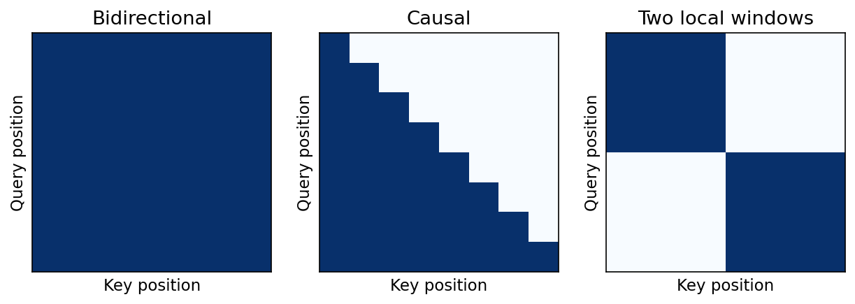
In cross-attention, queries come from one sequence and keys and values from another sequence : , , . The score matrix has shape , and the output has one row per query. This is how the original Transformer decoder reads its encoder, how image captioners read image features, and how text-to-image diffusion models read a text prompt (ML 08) without being autoregressive over image patches.
Attention weights are part of a computation, not automatically an explanation. A large weight can multiply an uninformative value, and the residual and MLP paths also shape the output.
Positional information
Plain version. Content-only self-attention has no built-in position labels. Position embeddings, relative information or position-dependent masks supply structure.
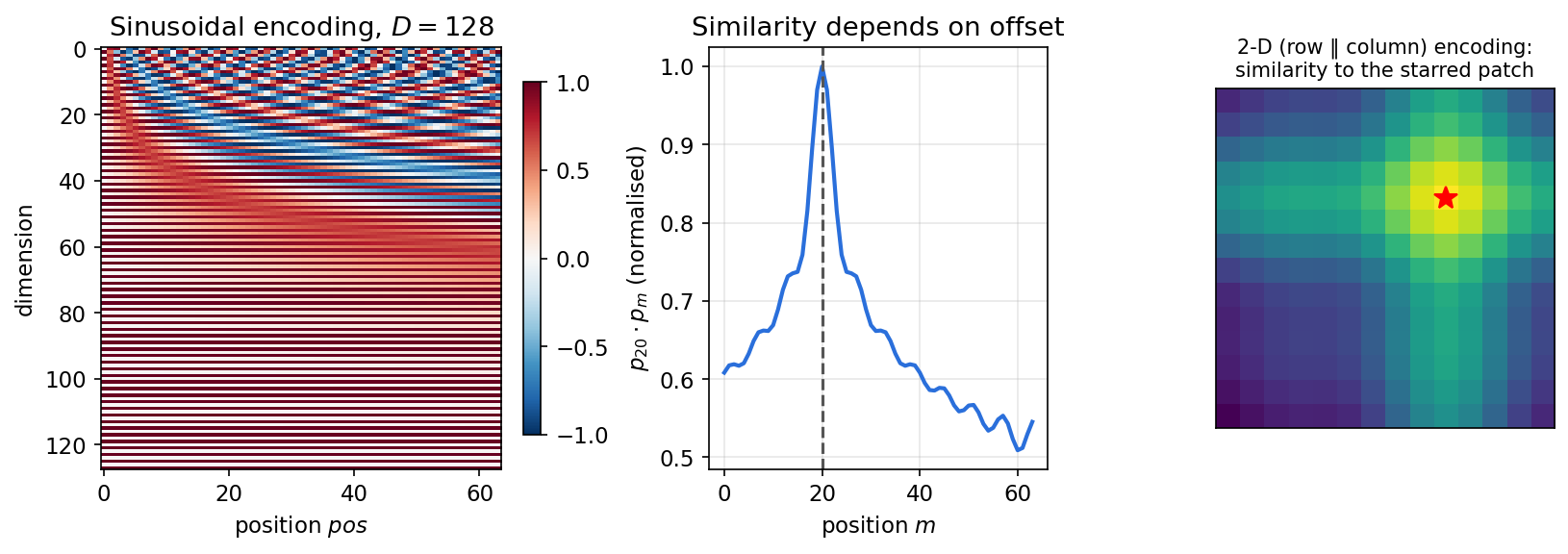
Sinusoidal encodings. The original Transformer [1] adds a fixed vector to the token at position :
Each pair of dimensions is a point rotating around a circle at angular frequency , from fast (one radian per position) to very slow. Two properties follow from the angle-addition formulas. First, for any fixed offset , for a block-diagonal rotation that does not depend on ; a linear layer can therefore learn to “look positions ahead”. Second, depends only on the offset (Figure 2, middle).
Code · Python · 20 lines
import numpy as np

def sinusoidal(n_pos, D):
    pos = np.arange(n_pos)[:, None]
    omega = 1.0 / 10000 ** (np.arange(0, D, 2) / D)    # one frequency per sin/cos pair
    pe = np.zeros((n_pos, D))
    pe[:, 0::2] = np.sin(pos * omega)
    pe[:, 1::2] = np.cos(pos * omega)
    return pe, omega

pe, omega = sinusoidal(100, 16)
k = 7                                                 # a fixed offset
# block-diagonal rotation that maps p_pos to p_{pos+k}, the same for every pos
R = np.zeros((16, 16))
for i, w in enumerate(omega):
    c, s = np.cos(w * k), np.sin(w * k)
    R[2 * i:2 * i + 2, 2 * i:2 * i + 2] = [[c, -s], [s, c]]
print("p[pos+k] == p[pos] @ R for all pos:", np.allclose(pe[:-k] @ R, pe[k:]))
print("dot products depend only on offset:",
      np.isclose(pe[10] @ pe[17], pe[50] @ pe[57]))
Both checks print True.
Other schemes.
- Learned absolute embeddings: a trainable vector per position, as in ViT [2]. ViT’s 1-D learned embeddings, indexed by raster order, worked about as well as explicitly 2-D ones; after training, embeddings of patches in the same row or column became similar, so the model learned the grid by itself. At a new resolution, the grid of embeddings is resized by 2-D interpolation before fine-tuning.
- Relative position representations (Shaw et al. [17]) add a learned term that depends on the offset to the score between tokens and . Swin [5] adds a learned relative position bias table to each window’s scores.
- Rotary position embedding (RoPE) (Su et al. [16]) rotates each query and key by an angle proportional to its position, using the same rotations as the sinusoidal code above. The score then depends on the positions only through . RoPE is standard in large language models and increasingly used in vision with separate rotations for the two image axes.
- No explicit encoding: convolutions inside the network, as in CvT [19], or zero padding at borders can leak enough position information on their own.
The Transformer block
Plain version. A block alternates two jobs. Attention lets tokens exchange information; a small MLP then processes each token on its own. Residual connections and normalization keep the stack stable.
Precise version. The pre-norm block used by ViT and most modern models is
is layer normalization [14]: it standardizes each token’s features to zero mean and unit variance, then applies a learned scale and shift; unlike BatchNorm, it does not depend on other samples in the batch. The MLP expands each token from to typically hidden units, applies the GELU nonlinearity [26] (, where is the standard normal CDF), and projects back. The residual additions mean each sub-layer only learns a correction, exactly as in ResNet.
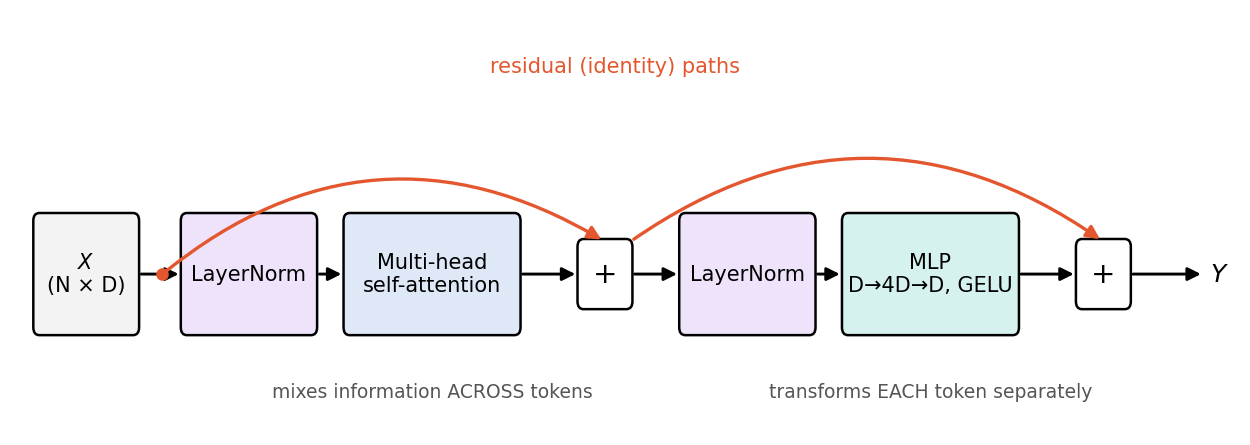
The original Transformer placed LayerNorm after each residual addition (post-norm). Xiong et al. [15] showed that with post-norm the gradients near the output are large at initialization, which is why it needs a learning-rate warm-up, whereas pre-norm keeps gradients well behaved and can train without one. So “a Transformer” is not fully specified until you say where the normalization goes. Counting weights per block: for attention and for the MLP, so about , two thirds of it in the MLP.
The Vision Transformer (ViT)
Plain version. Cut the image into square patches, turn each patch into a vector, add position information, and feed the sequence to a standard Transformer encoder. Read the answer from a special extra token.
Patchify. For an image with pixels and channels, and patch size dividing both and , there are patches. Flatten each into and project linearly:
where is the learned patch embedding, is a learned class token prepended to the sequence, and holds learned position embeddings. After blocks, a LayerNorm and a linear head applied to the class token’s output give the logits. Averaging all patch outputs (mean pooling) is an equally common alternative to the class token.
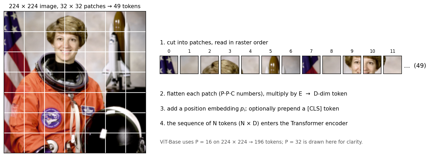
A linear map applied to non-overlapping patches is exactly a convolution with kernel size and stride both equal to , which is how implementations write it:
Code · Python · 20 lines
import torch
from torch import nn

torch.manual_seed(0)
B, C, H, W, P, D = 2, 3, 32, 32, 8, 48
x = torch.randn(B, C, H, W)

# 1) explicit: cut into P x P patches, flatten each, multiply by E
patches = x.unfold(2, P, P).unfold(3, P, P)                 # B, C, H/P, W/P, P, P
patches = patches.permute(0, 2, 3, 1, 4, 5).reshape(B, -1, C * P * P)   # B, N, P*P*C
E = torch.randn(C * P * P, D) * 0.02
tokens_explicit = patches @ E                                # B, N, D

# 2) the same linear map written as a convolution with kernel = stride = P
conv = nn.Conv2d(C, D, kernel_size=P, stride=P, bias=False)
conv.weight.data = E.T.reshape(D, C, P, P)
tokens_conv = conv(x).flatten(2).transpose(1, 2)             # B, N, D

print("tokens:", tuple(tokens_conv.shape), "| identical:",
      torch.allclose(tokens_explicit, tokens_conv, atol=1e-5))
It prints 16 tokens of width 48 and True.
Sizes. The standard configurations are ViT-Base (12 blocks, , 12 heads, about 86 million parameters), ViT-Large (24 blocks, , 16 heads) and ViT-Huge (32 blocks, , 16 heads) [2]. “ViT-B/16” means Base with patches. Patch size is the main compute knob: halving quadruples and multiplies the attention-score count by sixteen. Small patches keep fine detail; large patches are cheap but lose anything finer than the patch, which no later layer can recover.
The data lesson. Dosovitskiy et al. [2] found that ViT trained only on ImageNet-1k (about 1.3 million images) was somewhat worse than comparable ResNets, but when pretrained on ImageNet-21k (14 million) or JFT-300M (300 million) and then fine-tuned, it matched or exceeded them at lower pretraining cost. Their explanation is inductive bias: a CNN assumes locality and translation equivariance in every layer, whereas a ViT is local only within the patch embedding and must learn spatial relationships from data. Raghu et al. [18] compared the internal representations of ViTs and ResNets and found that ViTs have more uniform representations across layers, that their lower layers attend both locally and globally, and that learning local attention in early layers requires large-scale pretraining.
Code: a tiny ViT trained on digits
This complete example trains a small ViT on the same digits as the CNN in ML 03, with patches (16 tokens), a class token, learned positions and four pre-norm blocks. It runs on CPU in about half a minute.
Code · Python · 52 lines
import copy
import numpy as np
import torch
from torch import nn
from sklearn.datasets import load_digits
from sklearn.model_selection import train_test_split

torch.manual_seed(0)
torch.set_num_threads(1)

class TinyViT(nn.Module):
    def __init__(self, img=8, patch=2, chans=1, D=64, depth=4, heads=4, classes=10):
        super().__init__()
        N = (img // patch) ** 2
        self.patch = nn.Conv2d(chans, D, kernel_size=patch, stride=patch)   # patchify + E
        self.cls = nn.Parameter(torch.zeros(1, 1, D))                       # [CLS] token
        self.pos = nn.Parameter(torch.randn(1, N + 1, D) * .02)             # learned positions
        layer = nn.TransformerEncoderLayer(D, heads, dim_feedforward=4 * D, dropout=0.1,
                                           activation="gelu", batch_first=True,
                                           norm_first=True)                 # pre-norm block
        self.blocks = nn.TransformerEncoder(layer, depth, enable_nested_tensor=False)
        self.norm, self.head = nn.LayerNorm(D), nn.Linear(D, classes)

    def forward(self, x):
        t = self.patch(x).flatten(2).transpose(1, 2)                         # B, N, D
        t = torch.cat([self.cls.expand(len(t), -1, -1), t], dim=1) + self.pos
        return self.head(self.norm(self.blocks(t))[:, 0])                    # read [CLS]

d = load_digits()
X = torch.tensor(d.images[:, None] / 16.0, dtype=torch.float32)
y = torch.tensor(d.target)
train, test = train_test_split(np.arange(len(y)), test_size=.2, stratify=d.target,
                               random_state=0)
train, val = train_test_split(train, test_size=.2, stratify=d.target[train], random_state=1)
model = TinyViT()
opt = torch.optim.AdamW(model.parameters(), lr=1e-3, weight_decay=0.05)
best = (float("inf"), None)
for epoch in range(30):
    model.train()
    for idx in torch.tensor(train)[torch.randperm(len(train))].split(64):
        loss = nn.functional.cross_entropy(model(X[idx]), y[idx])
        opt.zero_grad(); loss.backward(); opt.step()
    model.eval()
    with torch.no_grad():
        v = nn.functional.cross_entropy(model(X[val]), y[val]).item()
    if v < best[0]:
        best = (v, copy.deepcopy(model.state_dict()))
model.load_state_dict(best[1]); model.eval()
with torch.no_grad():
    acc = (model(X[test]).argmax(1) == y[test]).float().mean().item()
print("parameters:", sum(p.numel() for p in model.parameters()))
print("best validation loss:", round(best[0], 4), "| held-out accuracy:", round(acc, 4))
On our run it uses about 202,000 parameters and reaches about 95% held-out accuracy, while the CNN in ML 03 reached about 96% with fewer than 10,000 parameters and the same split. On a small dataset, the CNN’s built-in locality is worth a factor of twenty in parameters. This is the data lesson in miniature, not a verdict on large-scale performance.
Optional: ViT (in the Paper guides). Read the original figure, evidence, design choices and limitations.
Training recipes: DeiT and beyond
Plain version. Much of the early gap between ViTs and CNNs on ImageNet-sized data turned out to be about training, not architecture.
DeiT (Touvron et al. [4]) trained ViTs competitively on ImageNet-1k alone using strong data augmentation (RandAugment, Mixup, CutMix, random erasing), heavy regularization (stochastic depth, label smoothing) and long schedules. It also introduced a distillation token: an extra learned token, like the class token, whose output is trained to match the predictions of a pretrained CNN teacher. The CNN’s inductive bias is thus transferred through its predictions. DeiT III [27] later showed that a simpler, carefully tuned supervised recipe (a lightweight “3-Augment” scheme, simple cropping and a binary cross-entropy loss) makes plain ViTs stronger still. Steiner et al. [25] ran a large study of data, augmentation and regularization (“AugReg”) and found that the right combination of augmentation, regularization and compute can match models trained on roughly ten times more data.
The general lesson, repeated in ML 03’s discussion of ConvNeXt: compare architectures only under matched data, augmentation, resolution, schedule and compute.
Swin and hierarchical Transformers
Plain version. Global attention over thousands of tokens is expensive, and plain ViT keeps one coarse resolution throughout, which is awkward for detection and segmentation. Swin restricts attention to local windows, shifts the windows between layers so information still spreads, and merges patches to build a CNN-like pyramid.
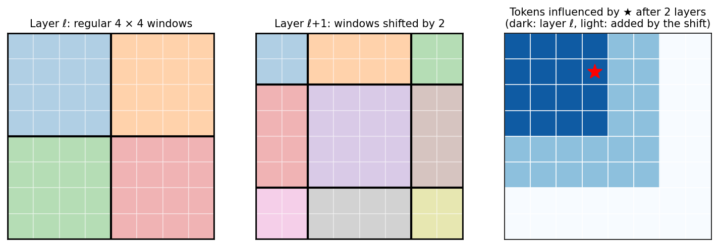
Windows. Swin [5] partitions the token grid into non-overlapping windows of tokens (typically ) and computes self-attention inside each window only. For an token grid with channels, the paper gives the costs
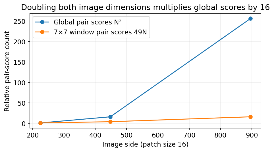
where counts the four projections and the second term counts the score and weighting products. Global cost is quadratic in the number of tokens ; window cost is linear for fixed .
Shifted windows. With fixed windows, tokens in different windows would never interact. Swin alternates regular windows with windows displaced by tokens in each direction. A token near a window boundary at layer shares a window with tokens from neighboring windows at layer , so information crosses boundaries (Figure 5). An efficient implementation cyclically shifts the feature map and uses a mask so that tokens wrapped from opposite edges do not attend to each other.
Hierarchy. Between stages, patch merging concatenates each group of neighboring tokens and projects them linearly, halving the resolution and doubling the channels, as a strided convolution would. The four stages produce feature maps at , , and of the input resolution, the same pyramid a ResNet produces, so Swin can replace a CNN backbone in detection and segmentation frameworks. Each window also adds a learned relative position bias to its scores. Swin V2 [32] scaled the design up with residual post-normalization, scaled cosine attention and a continuous, log-spaced position bias that transfers better across window sizes and resolutions.
Hybrid CNN–Transformer models
Plain version. Convolutions are good at local detail with little data; attention is good at long-range interaction. Hybrids use each where it helps.
- Convolutional stem. The original ViT paper already tested a “hybrid” in which the patches come from a ResNet feature map instead of raw pixels [2]; it helped at smaller compute budgets.
- Convolutions inside attention. CvT [19] uses a convolutional token embedding at each stage and depthwise-convolutional projections for queries, keys and values, which builds in locality and lets it drop explicit position embeddings.
- Stacking by stage. CoAtNet [20] places depthwise-convolution stages early, where resolution is high and local patterns dominate, and relative-attention stages later; it reports strong results across data scales because the convolutional stages supply inductive bias when data is limited.
- Mobile hybrids. MobileViT [28] inserts small Transformer blocks into a MobileNet-style network to add global context at mobile cost.
- The reverse direction. ConvNeXt (see ML 03) imported Transformer-era design choices into a pure CNN and matched Swin.
Cost and efficient attention
Plain version. Global attention compares token pairs, so its pairwise work grows quadratically with token count. Efficiency methods reduce memory traffic, interactions or token count.
For tokens of width , the score matrix costs about multiply–adds per layer and the projections and MLP about . A naive implementation stores an matrix per head. Doubling the image height and width at a fixed patch size multiplies by four and the pairwise scores by sixteen.
The main families:
- Exact but faster. FlashAttention [6] computes exact attention by tiling the computation so that blocks of queries, keys and values stay in fast on-chip memory, and never writes the full matrix to slow GPU memory; FlashAttention-2 [29] improves the work partitioning further. The arithmetic is still quadratic; the memory is linear and wall-clock time drops substantially. PyTorch’s
scaled_dot_product_attentionselects such kernels automatically when it can [7]. - Restricted connectivity. Windowed (Swin) or other sparse patterns reduce the number of pairs, at the price of needing several layers for global communication.
- Fewer tokens. Token Merging (ToMe) [21] gradually merges similar tokens inside a pretrained ViT using a fast matching step, increasing throughput without retraining. Larger patches, token pruning and pooling stages do the same more bluntly.
- Smaller models. Papa et al.’s survey [13] organizes efficient ViTs into compact architectures, pruning, knowledge distillation and quantization, and proposes an “Efficient Error Rate” metric to compare models across parameters, bits, FLOPs and size.
State-space models and hybrids
Plain version. Instead of comparing every pair of tokens, carry a compact state through the sequence, as a recurrent network does (ML 04). The cost grows linearly with the number of tokens.
A simplified state-space recurrence over a token sequence is
where is a hidden state of fixed size, and , , are (discretized) state-space matrices. In selective models such as Mamba, the write/read coefficients and step sizes depend on input ; the underlying continuous transition can remain fixed while its discretization varies. Input selection and an affine state update permit a parallel scan [33]. An image has no natural one-dimensional order, so vision variants must choose scan orders: Vision Mamba (Vim) [30] scans the patch sequence forward and backward with position embeddings, and VMamba [31] scans along four directions over the 2-D grid. The Visual Mamba survey [8] reviews over 200 papers and identifies scanning as the critical design decision for vision.
A useful counterpoint is MambaOut [9] (CVPR 2025). Its authors argue that Mamba suits tasks with long sequences and causal (autoregressive) structure, and build MambaOut models by removing the state-space component while keeping the gated convolutional blocks. Their models outperform visual Mamba models on ImageNet classification, suggesting that Mamba is unnecessary there, while for detection and segmentation, which involve long token sequences, they find state-space models may still be worth exploring. The broader point is methodological: isolate the mechanism (attention, scan, convolution) from gating, normalization, training recipe and parameter budget before crediting a result to it.
An image scan is an inductive bias
Mamba [33] supplies an efficient sequence operator; it does not choose an image geometry for us. Vim [30] uses a patch sequence, position embeddings and forward/backward processing. VMamba [31] instead places a four-route selective scan inside a hierarchical visual backbone. Neither label alone specifies receptive-field strength, resolution behavior or runtime. The state dimensions, routes, local operators and downsampling stages all matter.
For a fixed scan order, two adjacent pixels in the image may be many steps apart in the sequence. Conversely, the last pixel of one raster row and the first pixel of the next row become consecutive despite being far apart spatially. A local convolution can supply nearby evidence before the scan carries context farther. Multiple routes offer additional paths, but do not restore every geometric symmetry automatically. Position embeddings can also encode useful location while making transfer to a different grid a separate design problem.
A mathematical way to expose the choice is
Here contains flattened image tokens, indexes one of routes, permutes tokens into that route, applies its sequence recurrence, restores image coordinates, and averages the resulting features. This is a conceptual route-fusion model. A learned vision block can use different projections or fusion rules; averaging is chosen here to keep the experiment interpretable.
CPU experiment: measure directional bias
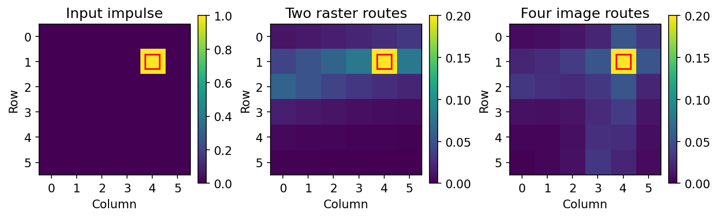
The next example uses a single scalar state with the same decay on every route. It compares forward/backward raster scans with four raster/column routes, then rotates the input by 90 degrees, processes it and rotates the output back. Everything uses a synthetic impulse; no weights or images are downloaded. This isolates ordering rather than reproducing a trained Vim or VMamba.
Code · Python · 28 lines
import numpy as np

def scan_image(image, four=False):
    ids = np.arange(image.size).reshape(image.shape)
    row, col = ids.ravel(), ids.T.ravel()
    orders = [row, row[::-1]]
    if four:
        orders += [col, col[::-1]]
    outputs = []
    for order in orders:
        h = 0.0
        out = np.zeros(image.size)
        for i in order:
            h = 0.8 * h + 0.2 * image.ravel()[i]
            out[i] = h
        outputs.append(out.reshape(image.shape))
    return np.mean(outputs, axis=0)

image = np.zeros((6, 6))
image[1, 4] = 1.0
errors = []
for four in [False, True]:
    original = scan_image(image, four=four)
    rotated_back = np.rot90(scan_image(np.rot90(image), four=four), -1)
    error = np.max(np.abs(original - rotated_back))
    errors.append(error)
    print('four routes:', four, 'rotation discrepancy:', round(error, 6))
assert 0.0 < errors[1] < errors[0]
The maximum discrepancies are 0.063622 for two routes and 0.026738 for four. More routes reduce directional bias in this example, but the remaining discrepancy is nonzero. Rotating a raster path reverses one traversal axis; that path need not belong to the original four-route collection. Even shared coefficients and averaging therefore do not guarantee rotation equivariance. Learned directional projections, position information and local operations introduce further choices. Test the property you need instead of inferring it from “2-D scan.”
The recurrence can have a global receptive field because information travels through the entire scan. This says a dependence is possible, not that its influence remains strong at every distance. With scalar decay , the carried contribution decays by another factor of per intervening step. Selective transitions can change this retention, as derived in ML 04, but training must still learn which information to preserve. Fine boundaries and small objects can be lost through state compression or downsampling even when distant context is available.
What Mamba-2 changes, and how to evaluate it
Mamba-2 [34] reorganizes the selective sequence mixer around structured state-space duality and efficient chunk computation. It changes the transition structure and block parameter projections, rather than making an arbitrary image patch sequence equivalent to a Transformer. The causal structured coefficient matrix has an attention-like interpretation, but standard softmax attention retains different expressive and computational properties. An image application must still specify directions and fusion. The duality therefore answers a computation question; it does not remove the geometry question.
A fair vision comparison should separate three experiments: replace only the mixer inside a shared block; compare complete backbones under a matched training budget; and measure the deployed models on the target hardware. Keep data, augmentation, token resolution and downstream heads controlled. Record state size as well as parameter count, and measure latency and peak memory across image resolutions and batch sizes. A linear token-count term can coexist with expensive projections, route permutations and small-kernel overheads. GPU throughput claims do not follow from the Python loop above.
For dense tasks, inspect errors near boundaries, on small structures and across aspect ratios; for video, distinguish an offline bidirectional encoder from causal live processing. Include rotation/crop sensitivity and longer-grid evaluations rather than only in-distribution classification. MambaOut [9] supplies an important mixer-removal ablation. Its results support a task-dependent comparison, not a theorem that scans are unnecessary for every image problem. Xu et al. [8] organize visual Mamba work by backbones, scan mechanisms and image/video/point-cloud/multimodal applications. Their survey remains a 2024 preprint on the verified record. Its taxonomy is useful for selecting controlled experiments; the number of proposed variants does not establish a universal winner.
Modern view
Survey literature. Khan et al. [3] (ACM Computing Surveys, 2022) start from the foundations (self-attention, large-scale pretraining, bidirectional encoding) and then survey Transformers across recognition, generative modeling, multimodal tasks such as visual question answering, video, low-level vision and 3-D analysis, closing with open problems. Han et al. [11] (IEEE TPAMI, 2023) organize vision Transformers by task (backbones, high- and mid-level vision such as detection and segmentation, low-level vision, video), and also cover efficient Transformer methods. Liu et al. [12] (IEEE TNNLS, 2024) review over a hundred visual Transformers for classification, detection and segmentation on images, point clouds and vision–language data, and suggest three future directions. For efficiency, Papa et al. [13] (IEEE TPAMI, 2024) is the most systematic. For state-space vision models, see Xu et al. [8]. Bishop and Bishop [10] provide the textbook derivations.
State of the art, 2023–2026. The plain ViT has become the default foundation backbone. ViT-22B [24] (ICML 2023) scaled a ViT to 22 billion parameters, with architectural changes (such as normalizing queries and keys) needed for stable training at that size. DINOv2 [23] (TMLR 2024) trained ViTs with self-supervision on a large curated image collection and produced general-purpose features that work frozen across classification, segmentation and depth estimation (ML 06). Darcet et al. [22] (ICLR 2024) found that large ViTs repurpose uninformative background patches as internal scratch space, producing high-norm artifact tokens in attention maps, and that adding a few extra register tokens removes the artifacts and improves dense predictions. Vision–language foundation models (ML 10) and diffusion Transformers (ML 08) build on the same block. At the same time, hierarchical and hybrid designs remain common for dense, high-resolution tasks, modernized CNNs remain competitive under matched budgets (ML 03), and state-space and linear-attention models continue to be explored for very long token sequences such as video.
Open problems. Quadratic cost at high resolution and long video; the large data and compute appetite of plain ViTs; position encodings that generalize across resolutions and aspect ratios; interpreting attention without over-reading it; and fair, compute-matched comparisons between attention, convolution and state-space mechanisms.
Key takeaways
- Queries and keys determine weights; values provide the content mixed by attention.
- Score scaling controls magnitude under variance assumptions; it does not guarantee unit variance for arbitrary learned inputs.
- Masks constrain information access, while positional signals distinguish arrangements that content-only attention cannot.
- Transformer blocks alternate token mixing and per-token transformations, with residual paths and normalization.
- ViT, shifted windows and convolutional hybrids make different choices about locality, resolution and training requirements.
- FlashAttention reduces memory traffic for exact attention; windows, token reduction and state-space scans alter computation or context access.
Exercises
- Token budget. Calculate the number of tokens and attention-score entries per head for a image with patches of size 16 and 8. By what factor does the score count grow when the patch size halves?
Hint
and tokens; and scores. Halving the patch size multiplies by 4 and the scores by 16.
- Scaling check. Draw random queries and keys with independent standard-normal components for . Measure the variance of with and without division by , and the largest softmax weight over 100 keys in each case. What happens to the softmax without scaling?
Hint
The variance of the raw dot product is close to ; after scaling it is close to 1. Without scaling, at the softmax puts nearly all weight on a single key (it becomes almost one-hot), so gradients through the other keys vanish.
- Remove position. In the TinyViT code, set the position embeddings to zero, drop the class token and use mean pooling, then permute the patch tokens before the blocks and compare the logits in evaluation mode. Explain the result, and what it implies for an image classifier without positional information.
Hint
The logits agree up to floating-point error, because every block is permutation-equivariant and mean pooling is permutation-invariant. Use dropout off (eval()) and permute tokens, not pixels inside a patch. Such a model cannot tell a face from a scrambled face built from the same patches.
- Cross-attention shapes. In a text-to-image model, 256 image tokens of width 320 read 77 text tokens of width 768 with 8 heads of width 40. Give the shapes of , , , one head’s score matrix, and the output.
Hint
(8 heads × 40), . Each head’s scores are . The output follows the queries: after the output projection. Key and value lengths must match each other, not the query length.
- Swin arithmetic. Using the cost formulas, compare global and window attention for a token grid with and . Which term dominates in each case?
Hint
. Global: plus , so the quadratic term dominates. Window: the same plus , so the projections dominate. The window version is about 14 times cheaper here.
- Fair comparison. You have 2,000 labeled images and access to pretrained CNN, ViT and visual Mamba backbones. Design an experiment that tells you which backbone to deploy, and list what must be held fixed. Include a mixer-removal ablation and a resolution/rotation test.
Hint
Compare linear probes on frozen features first, then fine-tuning with matched budgets and tuned learning rates per model on a validation split. Record pretraining data, input resolution, parameters, FLOPs and measured latency on the target device. A pretrained ViT against a CNN trained from scratch tests pretraining, not architecture. For the scan backbone, record state size and test whether benefits survive removing the mixer while retaining gating and local convolution. Keep the same preprocessing in the resolution and rotation tests.
References
- A. Vaswani et al., “Attention Is All You Need,” NeurIPS, 2017. arXiv
- A. Dosovitskiy et al., “An Image is Worth 16x16 Words: Transformers for Image Recognition at Scale,” ICLR, 2021. arXiv
- S. Khan, M. Naseer, M. Hayat, S. W. Zamir, F. S. Khan and M. Shah, “Transformers in Vision: A Survey,” ACM Computing Surveys, 2022. arXiv
- H. Touvron et al., “Training data-efficient image transformers & distillation through attention,” ICML, 2021. arXiv
- Z. Liu et al., “Swin Transformer: Hierarchical Vision Transformer using Shifted Windows,” ICCV, 2021. arXiv
- T. Dao, D. Y. Fu, S. Ermon, A. Rudra and C. Ré, “FlashAttention: Fast and Memory-Efficient Exact Attention with IO-Awareness,” NeurIPS, 2022. arXiv
- PyTorch,
scaled_dot_product_attentionandTransformerEncoderLayerdocumentation. Attention, Encoder layer MultiheadAttention mask semantics - R. Xu et al., “Visual Mamba: A Survey and New Outlooks,” arXiv:2404.18861, 2024. arXiv
- W. Yu and X. Wang, “MambaOut: Do We Really Need Mamba for Vision?,” CVPR, 2025. Paper
- C. M. Bishop and H. Bishop, Deep Learning: Foundations and Concepts, Springer, 2024, ch. 12. Book
- K. Han et al., “A Survey on Vision Transformer,” IEEE Transactions on Pattern Analysis and Machine Intelligence, 2023. DOI
- Y. Liu et al., “A Survey of Visual Transformers,” IEEE Transactions on Neural Networks and Learning Systems, 2024. DOI
- L. Papa, P. Russo, I. Amerini and L. Zhou, “A Survey on Efficient Vision Transformers: Algorithms, Techniques, and Performance Benchmarking,” IEEE Transactions on Pattern Analysis and Machine Intelligence, 2024. DOI
- J. L. Ba, J. R. Kiros and G. E. Hinton, “Layer Normalization,” arXiv:1607.06450, 2016. arXiv
- R. Xiong et al., “On Layer Normalization in the Transformer Architecture,” ICML, 2020. arXiv
- J. Su, M. Ahmed, Y. Lu, S. Pan, W. Bo and Y. Liu, “RoFormer: Enhanced Transformer with Rotary Position Embedding,” Neurocomputing, 2024. DOI
- P. Shaw, J. Uszkoreit and A. Vaswani, “Self-Attention with Relative Position Representations,” NAACL, 2018. arXiv
- M. Raghu, T. Unterthiner, S. Kornblith, C. Zhang and A. Dosovitskiy, “Do Vision Transformers See Like Convolutional Neural Networks?,” NeurIPS, 2021. arXiv
- H. Wu et al., “CvT: Introducing Convolutions to Vision Transformers,” ICCV, 2021. arXiv
- Z. Dai, H. Liu, Q. V. Le and M. Tan, “CoAtNet: Marrying Convolution and Attention for All Data Sizes,” NeurIPS, 2021. arXiv
- D. Bolya et al., “Token Merging: Your ViT But Faster,” ICLR, 2023. arXiv
- T. Darcet, M. Oquab, J. Mairal and P. Bojanowski, “Vision Transformers Need Registers,” ICLR, 2024. arXiv
- M. Oquab et al., “DINOv2: Learning Robust Visual Features without Supervision,” Transactions on Machine Learning Research, 2024. arXiv
- M. Dehghani et al., “Scaling Vision Transformers to 22 Billion Parameters,” ICML, 2023. arXiv
- A. Steiner et al., “How to train your ViT? Data, Augmentation, and Regularization in Vision Transformers,” Transactions on Machine Learning Research, 2022. arXiv
- D. Hendrycks and K. Gimpel, “Gaussian Error Linear Units (GELUs),” arXiv:1606.08415, 2016. arXiv
- H. Touvron, M. Cord and H. Jégou, “DeiT III: Revenge of the ViT,” ECCV, 2022. arXiv
- S. Mehta and M. Rastegari, “MobileViT: Light-weight, General-purpose, and Mobile-friendly Vision Transformer,” ICLR, 2022. arXiv
- T. Dao, “FlashAttention-2: Faster Attention with Better Parallelism and Work Partitioning,” ICLR, 2024. arXiv
- L. Zhu et al., “Vision Mamba: Efficient Visual Representation Learning with Bidirectional State Space Model,” ICML, 2024. arXiv
- Y. Liu et al., “VMamba: Visual State Space Model,” NeurIPS, 2024. arXiv
- Z. Liu et al., “Swin Transformer V2: Scaling Up Capacity and Resolution,” CVPR, 2022. arXiv
- A. Gu and T. Dao, “Mamba: Linear-Time Sequence Modeling with Selective State Spaces,” COLM, 2024. Author version
- T. Dao and A. Gu, “Transformers are SSMs: Generalized Models and Efficient Algorithms Through Structured State Space Duality,” ICML, PMLR 235, 2024. Paper
Check your understanding
This tutorial has 6 exercises. Can you solve them without opening the hints?
Go to the exercises ↑Next ML 06 · Representation Learning and Self-Supervision · 27 min