ML 10 · Foundation Models and Vision–Language Learning
Needs: ML 06 · Representation Learning and Self-Supervision, ML 09 · Autoregressive Vision: Pixels, Tokens and Scales, ML 08 · Diffusion Models and Flow Matching
Navigate: this page and this track: Navigate: this page and this track
On this page
- What you’ll learn1 min
- The big picture2 min
- What makes a model a “foundation” model1 min
- Scaling laws3 min
- Pre-training objectives: where does the target come from?4 min
- Image and text in a shared space: CLIP and SigLIP2 min
- Promptable segmentation: the Segment Anything family1 min
- Multimodal large language models3 min
- Adapting a foundation model5 min
- Video, geometry and world models1 min
- Risks and evaluation2 min
- Modern view2 min
- Key takeaways1 min
- Exercises2 min
- Paper guides
- References
Machine Learning
Explore this chapter 1 interactive experiment
Move paired and unpaired unit vectors, then inspect the normalized matching loss used by contrastive learning.
What you’ll learn
- Define foundation models through pretraining and reuse.
- Interpret scaling laws within their measured regimes.
- Compare supervision sources and reusable vision capabilities.
- Trace image–text alignment, visual prompts and multimodal connectors.
- Choose adaptation methods and test task performance, robustness and limitations.
The big picture
For most of the history of computer vision, each task had its own model: one network for classifying flowers, another for detecting cars, another for segmenting tumors, each trained from scratch or from an ImageNet [43] classifier. A foundation model is trained once, on broad data and at large scale, and then adapted to many downstream tasks [1]. The word describes how the model is trained and reused, not a new layer type. A DINOv2 [15] or DINOv3 [16] image encoder, a CLIP-style image–text model [3], a promptable segmenter such as SAM [5], a multimodal language model and a broadly pretrained image generator can all play this role.
Why does this matter? Three reasons. First, labels are expensive and pretraining moves most of the learning to data that needs no hand labels (captions, the images themselves). Second, one backbone serves many tasks, which concentrates engineering effort. Third, it changes the interface: instead of retraining, you can often specify a task with a text prompt, a click or a few examples. Bommasani et al. call the resulting concentration of methods homogenization, and warn that it also concentrates failure: a flaw in one shared backbone is inherited by every system built on it [1].
This chapter builds on ML 06 · Representation Learning (what makes a feature reusable), ML 05 · Vision Transformers (the usual backbone) and the generative chapters ML 08 and ML 09. The textbook treatment of transfer learning and representation in Bishop and Bishop [14] is a good companion. We follow the architectural map of the vision foundation-model survey by Awais et al. [39] and the multimodal survey by Caffagni et al. [2], with representative reports verified for this October 2026 edition. Examples illustrate families; they do not rank commercial products or claim that one checkpoint is best everywhere.
What makes a model a “foundation” model
Plain version. A foundation model is a large model pretrained on broad data with a generic objective, so that its internal representations or its interface can be reused for tasks it was never specifically trained on.
Bommasani et al. [1] coined the term in 2021 and emphasized two properties:
- Emergence. Capabilities arise from scale and the training objective rather than being designed explicitly. For example, CLIP was trained only to match images with captions, yet it can classify images into categories named in text [3]; DINO was trained without any labels, yet its attention maps outline objects [24].
- Homogenization. Many applications converge on a small number of pretrained backbones and recipes.
Be careful with “emergence”. In this chapter it means only a capability that was not a training target. It does not mean an unpredictable or mysterious jump; whether a capability appears suddenly often depends on the metric used to measure it.
Formally, let be a model pretrained on an upstream dataset with objective :
A downstream task supplies a (usually small) dataset and a task loss . Adaptation chooses a small set of new or changed parameters and solves
where is whatever we put on top of or inside the pretrained model: a linear head, an adapter, a LoRA update, a prompt, or nothing at all (pure prompting, ). The whole chapter is about the two lines above: what and should be, and how small can be.
A foundation model does not have to produce text. A frozen image encoder whose features feed a hundred different classifiers is a foundation model. Conversely, a large model trained for one narrow task is not one, however big it is.
Scaling laws
Plain version. Scaling laws fit how loss changes with model size, data and compute. They help plan runs within comparable regimes, but do not guarantee extrapolated gains.
Kaplan et al. [17] trained families of Transformer language models and reported that the loss scales as a power law in model size, dataset size and compute, with some trends spanning more than seven orders of magnitude, while width and depth mattered little within the tested range. A power law in model size reads
where is held-out cross-entropy loss, the number of non-embedding parameters, a fitted constant with the same units as , and the fitted exponent. Taking logs gives : a straight line with slope .
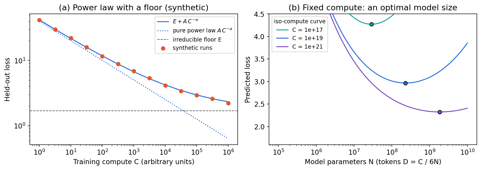
Real curves bend because some loss can never be removed (the data itself is noisy or ambiguous). Hoffmann et al. [18] therefore fitted a form with an irreducible term:
where is the number of training tokens, the irreducible loss, and fitted constants. For dense Transformers a common approximation of training compute is floating-point operations [17] (roughly two for the forward and four for the backward pass, per parameter per token). Fixing and minimizing over (with ) gives a compute-optimal model size. Hoffmann et al. trained over 400 language models and concluded that, for compute-optimal training, model size and training tokens should be scaled equally — every doubling of model size should come with a doubling of tokens [18]. That differed from Kaplan et al.’s earlier recommendation of very large models trained on relatively modest data [17]; the disagreement is a useful reminder that fitted exponents depend on the experimental protocol (learning-rate schedules, which runs are included, what is counted as compute).
Vision has its own scaling studies. Zhai et al. [19] characterized the relationship between error rate, data and compute for Vision Transformers [21] trained on large labeled datasets, scaling to two-billion-parameter models. Cherti et al. [20] trained CLIP-style models on the public LAION dataset [34] and found power-law scaling for zero-shot classification, retrieval, linear probing and fine-tuning — but also that OpenAI’s CLIP and OpenCLIP, with the same architectures and similar recipes, scale differently because their training distributions differ. Data is not a scalar.
Code: fit a scaling law and extrapolate
The snippet fits to the cheaper of 13 synthetic training runs and then predicts the expensive ones. Everything is synthetic; the point is the procedure.
Code · Python · 22 lines
import numpy as np
from scipy.optimize import curve_fit

rng = np.random.default_rng(0)
# Synthetic "runs": loss = E + A * C^(-alpha), with 2% multiplicative noise.
E_true, A_true, alpha_true = 1.7, 40.0, 0.3
compute = np.logspace(0, 6, 13)            # arbitrary compute units
loss = (E_true + A_true * compute**-alpha_true) * np.exp(.02 * rng.normal(size=13))

def law(c, E, A, alpha):
    return E + A * c**-alpha

# Fit only the cheaper runs, then extrapolate to the larger ones.
small = compute <= 1e4
(E, A, alpha), _ = curve_fit(law, compute[small], loss[small], p0=(1, 10, .5))
print(f"fit: E={E:.2f}  A={A:.1f}  alpha={alpha:.3f}")
for c, l in zip(compute[~small], loss[~small]):
    print(f"C={c:9.0f}  observed {l:.3f}  predicted {law(c, E, A, alpha):.3f}")

# Naive straight line in log-log space ignores the floor E.
slope = np.polyfit(np.log(compute[small]), np.log(loss[small]), 1)[0]
print(f"pure power-law slope without floor: {slope:.3f}")
Output: the fit recovers , , ; the extrapolated losses are within about 7% of the noisy observations; and a straight log–log line without the floor gives a slope of about , a wrong exponent. Two lessons transfer to real practice: always include the floor, and treat extrapolation over many orders of magnitude as a forecast with error bars.
What scaling laws do not tell you
- They predict average loss on the pretraining distribution, not accuracy on your task. Downstream metrics may improve smoothly, saturate, or move in steps.
- They hold for a fixed recipe and data distribution [20]. Better data filtering or a different objective changes the constants.
- They say nothing about inference cost. A smaller model trained on more data can be cheaper to deploy at the same loss, which is why many deployed models are trained beyond the compute-optimal point.
- Data is finite. If the high-quality data runs out, the term stops shrinking however much compute you add.
Pre-training objectives: where does the target come from?
Plain version. Every pretraining method invents a prediction task. The difference is where the “answer” comes from: a human label, a caption, a hidden part of the same image, another network, or the next token.
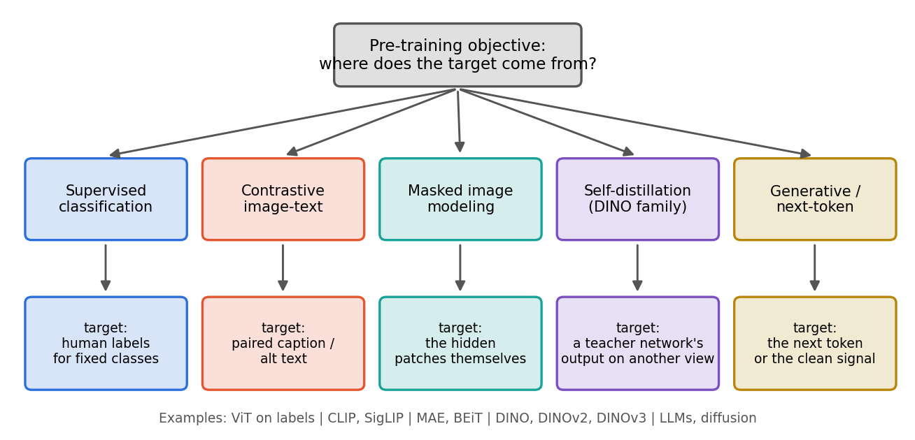
| Objective | Target comes from | Representative models | Typical strength |
|---|---|---|---|
| Supervised classification | Human labels | ViT on large labeled sets [19], [21] | Strong global semantics for the label space |
| Contrastive image–text | Paired captions / alt text | CLIP [3], ALIGN [25], SigLIP [4] | Text-defined recognition, retrieval |
| Masked image modeling | Hidden patches of the same image | BEiT [23], MAE [22] | Strong after fine-tuning; local detail |
| Self-distillation | A teacher network’s output on another view | DINO [24], DINOv2 [15], DINOv3 [16] | Frozen features, dense correspondence |
| Generative / next-token | Next token or clean signal | LLMs, diffusion (ML 07), AR (ML 08) | Generation; language interface |
Supervised pre-training
Train a classifier with cross-entropy on a large labeled dataset, then drop the final layer. This was the ImageNet recipe for a decade and still works at scale [19], [21]. Its weakness is that the features are shaped by a fixed label set: distinctions that the labels do not require may be discarded.
Contrastive image–text learning
Captions come for free with web images, so CLIP [3] and ALIGN [25] train an image encoder and a text encoder together so that matching pairs score higher than mismatched ones within a batch. ALIGN showed that a large, noisy alt-text corpus with minimal filtering can still give strong representations [25]. The loss is detailed in the next section.
Masked image modeling
Hide most of an image and predict what is missing. BEiT [23] masks patches and predicts discrete visual tokens for them, borrowing the masked-language-modeling idea from BERT [44]. MAE [22] predicts the raw pixels directly and observes that masking a high proportion, e.g. 75% of patches, creates a nontrivial task; its encoder sees only the visible patches and a lightweight decoder reconstructs the rest, which makes training efficient. With the set of masked patch indices, the (normalized) pixels of patch and the reconstruction,
The loss is computed only on masked patches: predicting the visible ones would be trivial copying. Masked-modeling features are often excellent after fine-tuning but weaker as frozen features for linear probing than contrastive or self-distilled ones.
Self-distillation: the DINO family
DINO [24] — described by its authors as self-distillation with no labels — trains a student network to match a teacher network on different augmented views (crops) of the same image. Both output -dimensional scores; probabilities are softmaxes with temperatures and :
Here and are two views, is a running mean of teacher outputs (centering), and a small makes the teacher’s distribution sharp (sharpening). Centering stops one dimension from dominating; sharpening stops the output from becoming uniform; together they avoid collapse, the trivial solution where every image maps to the same output. The teacher receives no gradients. Its weights are an exponential moving average (the momentum encoder) of the student’s:
DINO also uses multi-crop training (several small local crops for the student, global crops for the teacher), which forces local-to-global correspondence. Its authors report that the resulting ViT features contain explicit information about object segmentation that does not emerge as clearly with supervised ViTs or convnets, and that they work well as k-nearest-neighbor classifiers [24].
DINOv2 [15] scales this recipe and, crucially, curates the data: an automatic pipeline builds a dedicated, diverse, curated image dataset instead of using uncurated web images, a 1-billion-parameter ViT is trained, and it is distilled into smaller models. The authors report that these frozen features surpass OpenCLIP on most of their image-level and pixel-level benchmarks [15]. DINOv3 [16] scales data and model further and introduces Gram anchoring, a technique aimed at a known problem: dense (per-patch) feature maps degrading during long training schedules. It also adds post-hoc strategies for flexibility in resolution, model size and alignment with text.
Why dense features matter. A classifier needs one vector per image. Segmentation, depth estimation, correspondence and tracking need a good vector per patch. Self-distilled encoders are popular frozen backbones for these dense tasks precisely because their patch features stay semantically meaningful without fine-tuning.
Generative pre-training
Predicting the next token (language models, autoregressive image models in ML 09) or denoising (diffusion in ML 08) is also a pretraining objective. For language it produces the most flexible interface — instructions in natural language — which is why multimodal models attach vision to a pretrained language model rather than the other way round.
Image and text in a shared space: CLIP and SigLIP
Plain version. Align paired image and text embeddings, then score images against candidate descriptions. Text-defined classification still depends on prompts and learned coverage.
CLIP [3] normalizes image embeddings and text embeddings to unit length and forms scores with a learned temperature . For a batch of paired examples,
Each image should select its matching caption among the captions (first term, a row-wise softmax), and each caption its matching image (second term, column-wise). All other pairs in the batch act as negatives. Training uses paired text supervision, usually from existing captions or alt text; “zero-shot” downstream use does not mean the model was trained without supervision.
At inference, encode candidate descriptions such as “a photo of a dog” and compare an image with them. The text embeddings replace the class weights of a learned classifier:
The candidate set and wording affect the result; averaging the embeddings of several templates (“a photo of a ”, “a close-up of a ”) is a common way to reduce sensitivity. Zero-shot means no task-specific parameter training under the stated protocol; it does not guarantee that the classes or even the test images were absent from pretraining (see Risks and evaluation).
Code: paired loss and retrieval mechanics
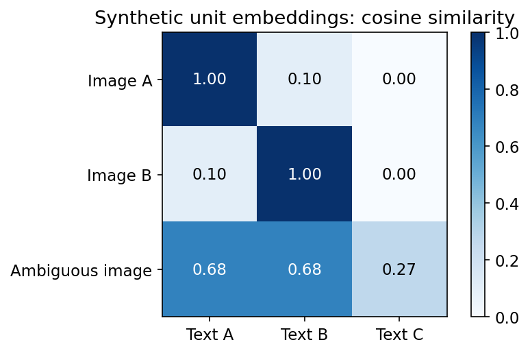
These synthetic embeddings make the computation transparent. They are not outputs from a pretrained model, and their matches do not demonstrate real-world zero-shot accuracy.
Code · Python · 14 lines
import torch
from torch.nn import functional as F

images = F.normalize(torch.tensor([[1., .1, 0.], [.1, 1., 0.],
                                   [0., .1, 1.]]), dim=-1)
texts = F.normalize(torch.eye(3), dim=-1)
scores = images @ texts.T / .1
labels = torch.arange(3)
loss = (F.cross_entropy(scores, labels) +
        F.cross_entropy(scores.T, labels))/2
print("matching text:", scores.argmax(1).tolist())
print("paired loss:", round(loss.item(), 4))
ambiguous = F.normalize(torch.tensor([[.5, .5, .2]]), dim=-1)
print("cosines:", (ambiguous @ texts.T).tolist())
It prints matching text: [0, 1, 2], a paired loss of about 0.0002, and cosines of about 0.68, 0.68, 0.27 for the ambiguous image: it is equally close to two descriptions, and no softmax can tell you which is right.
SigLIP: a sigmoid instead of a softmax
SigLIP [4] replaces the batch-normalized softmax with an independent binary decision for every image–text pair. With labels for matching pairs and otherwise, a learned scale and bias ,
where , so each term equals . Because no term needs a sum over the whole batch, the loss does not require a global normalization across devices, which simplifies large-batch training. Since there are positives and negatives, the bias is initialized so that the initial predictions are strongly negative.
Shared embeddings support retrieval and open-vocabulary recognition, but fine-grained counting, negation (“a dog without a collar”), spatial relations and rare domain terms are known weak points. Evaluate those requirements directly rather than inferring them from a strong overall classification score.
Optional: CLIP (in the Paper guides). Read the original figure, evidence, design choices and limitations.
Promptable segmentation: the Segment Anything family
Plain version. A prompt tells the model which region or concept you want, and the output is a mask.
SAM [5] combines a heavy image encoder (run once per image), a light prompt encoder and a light mask decoder, so many prompts can be answered quickly on the same image. Spatial prompts — points, boxes or rough masks — select objects without a fixed class vocabulary. Because a single click is ambiguous (a click on a shirt could mean the shirt or the whole person), SAM predicts several candidate masks with confidence scores. It was trained on SA-1B, over 1 billion masks on 11 million licensed and privacy-respecting images, collected with a model-in-the-loop data engine [5].
SAM 2 [6] extends promptable segmentation to video with a streaming memory: the model stores features of past frames and of the prompted object, and propagates the mask through time; corrective clicks on later frames update the memory.
SAM 3 [7], released in 2025 with a report revised in March 2026, introduces promptable concept segmentation: given a short noun phrase (e.g. “yellow school bus”), image exemplars, or both, it returns masks and identities for all matching instances. Its image-level detector and memory-based video tracker share one backbone, and a presence head decouples recognizing whether the concept occurs at all from localizing its instances [7].
These interfaces supply different information: a spatial point says where, a noun phrase says what, an exemplar says what it looks like. Report prompt creation cost and whether prompts come from people, ground truth or an automatic detector. A “zero-shot segmentation” score obtained with ground-truth boxes as prompts hides substantial annotation information.
Multimodal large language models
Plain version. Turn visual features into “words” a language model can read, then teach it to follow visual instructions.
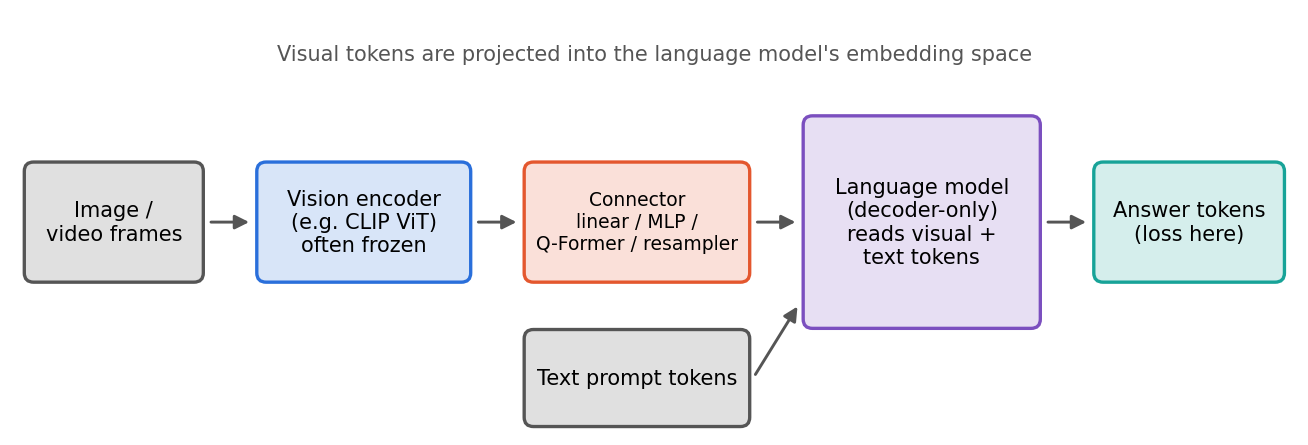
A common design has
Here is a grid of visual features (for a ViT, one vector per patch), is a sequence of vectors in the language model’s token-embedding space, and the decoder treats like the embeddings of ordinary words.
Connectors
- Linear or MLP projection. LLaVA [8] uses a single projection from CLIP features to the language model’s embedding space; LLaVA-1.5 [28] reports that a simple MLP connector (with a CLIP ViT-L at 336-pixel resolution and academic VQA data) is surprisingly powerful and data-efficient. Every patch becomes one visual token.
- Learned queries. BLIP-2 [26] inserts a lightweight Querying Transformer (Q-Former) between a frozen image encoder and a frozen language model. A fixed set of learned query vectors cross-attends to the image features, so the language model always sees a small, fixed number of visual tokens. BLIP-2 trains the Q-Former in two stages: representation learning against the frozen image encoder, then generative learning against the frozen language model.
- Resampling and cross-attention. Flamingo [27] bridges frozen vision and language models and handles arbitrarily interleaved sequences of images and text, which enabled few-shot learning from examples written directly in the prompt.
The trade-off is token count versus detail: one token per patch keeps fine detail but makes long sequences (expensive for many images or video); a few learned queries are cheap but can lose small text.
Visual instruction tuning
LLaVA [8] used a language-only GPT-4 [45] to generate multimodal instruction-following data from image captions and boxes, then trained in two stages: first align the connector (feature alignment), then fine-tune connector and language model on the instructions. The loss is ordinary next-token cross-entropy, applied to the answer tokens only:
where are text tokens, is the set of positions belonging to the assistant’s answer, and are the visual tokens. Instruction and prompt tokens are visible as context but masked out of the loss.
Qwen3-VL’s 2025 report [9] illustrates the current direction: a family of dense and mixture-of-experts models with natively interleaved image, video and text contexts of up to 256K tokens. It is a representative report, not evidence that every task benefits from longer contexts or more generated reasoning.
What the diagram hides
Reading a document may require preserving small text through tiling or dynamic resolution. Video questions need timestamps and temporal order. These details change token counts and preprocessing; a generic “vision encoder + LLM” diagram is only the starting point. A fluent answer can also contain objects that are not in the image (object hallucination) or wrong counts. Distinguish object grounding, OCR, spatial reasoning, factual answering and stylistic instruction following — they need different evidence and metrics (see Risks and evaluation). For a survey of the whole design space, see Yin et al. [40] and Caffagni et al. [2].
Adapting a foundation model
Plain version. Use the least expensive adaptation that solves the target task, and check it on data that looks like deployment.
| Strategy | Trainable components | Useful starting situation |
|---|---|---|
| Prompting / in-context examples | Nothing | The model’s interface already fits the task |
| Frozen features + linear head (linear probe) | Small supervised readout | Few labels, good feature transfer |
| Prompt tuning / visual prompt tuning | A few learned input tokens | Many tasks share one frozen backbone |
| Adapters / LoRA | Small inserted or low-rank modules | Domain adaptation under memory limits |
| Partial fine-tuning | Selected blocks plus head | Some adaptation without full optimizer cost |
| Full fine-tuning (optionally LP-FT) | All model parameters | Enough data and compute; transfer alone insufficient |
Linear probe
Freeze the encoder , compute features once, and fit a linear classifier . It is cheap, hard to overfit, and is also the standard measurement of representation quality: if a linear readout works, the information is linearly accessible in the features.
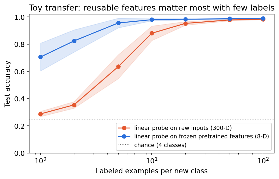
Code: why pretrained features help most with few labels
This toy experiment simulates the whole story. Observations are 300-dimensional and mix 8 semantic factors (which determine the class) with 8 large nuisance factors (think lighting and pose) plus noise. “Pretraining” sees 50 upstream classes with plenty of labels and learns an 8-dimensional projection (linear discriminant analysis, standing in for a deep encoder). Downstream, there are four new classes and only a few labels per class.
Code · Python · 35 lines
import numpy as np
from sklearn.discriminant_analysis import LinearDiscriminantAnalysis
from sklearn.linear_model import LogisticRegression

rng = np.random.default_rng(0)
D, k_sem, k_nui = 300, 8, 8
sem_map = rng.normal(size=(k_sem, D))   # semantic factors -> pixels
nui_map = rng.normal(size=(k_nui, D))   # nuisance factors (light, pose...)

def sample(centers, n):
    y = rng.integers(len(centers), size=n)
    z = centers[y] + 0.7 * rng.normal(size=(n, k_sem))
    u = 4.0 * rng.normal(size=(n, k_nui))          # large nuisance variation
    x = z @ sem_map + u @ nui_map + rng.normal(size=(n, D))
    return x, y

# 1) "Pre-training": many upstream classes with plenty of labels.
up_centers = rng.normal(size=(50, k_sem))
x_up, y_up = sample(up_centers, 10_000)
encoder = LinearDiscriminantAnalysis(n_components=k_sem).fit(x_up, y_up)

# 2) Downstream: four NEW classes, few labels, linear probe only.
new_centers = rng.normal(size=(4, k_sem))
x_te, y_te = sample(new_centers, 2_000)
f_te = encoder.transform(x_te)          # frozen features, computed once
for shots in [1, 5, 20, 100]:
    raw, feat = [], []
    for repeat in range(10):
        x_tr, y_tr = sample(new_centers, 4 * shots)
        raw.append(LogisticRegression(max_iter=3000)
                   .fit(x_tr, y_tr).score(x_te, y_te))
        feat.append(LogisticRegression(max_iter=3000)
                    .fit(encoder.transform(x_tr), y_tr).score(f_te, y_te))
    print(f"{shots:>3} labels/class | raw pixels {np.mean(raw):.3f}"
          f" | frozen features {np.mean(feat):.3f}")
On our machine it prints accuracies of roughly 0.29 vs 0.71 with one label per class, 0.62 vs 0.95 with five, 0.96 vs 0.99 with twenty and 0.98 vs 0.99 with a hundred (raw inputs vs frozen features; chance is 0.25). The pretrained projection already discards the nuisance directions, so a handful of labels suffice; with enough labels, the raw-input probe learns to ignore the nuisance itself and the gap closes. The upstream classes are different from the downstream ones — the features transfer because both share the same semantic factors. If the downstream task depended on a factor that pretraining threw away (here, the nuisance), frozen features would fail no matter how many labels you add. That is the failure mode to test for in practice.
Fine-tuning, LP-FT and robust fine-tuning
Full fine-tuning updates every weight and usually gives the best in-distribution accuracy when data suffices. But Kumar et al. [32] showed that it can distort good pretrained features: across their benchmarks, fine-tuning gave on average higher in-distribution but lower out-of-distribution accuracy than linear probing. Their explanation is that a randomly initialized head sends large, noisy gradients into the backbone early in training. LP-FT — first fit a linear probe, then fine-tune everything starting from that head — reduced this distortion and outperformed both alternatives in their experiments [32]. WiSE-FT [33] takes another route: linearly interpolate the weights of the zero-shot and fine-tuned models, , which improved robustness under distribution shift for CLIP-style models while keeping strong target accuracy. Both are cheap to try and worth knowing before declaring that fine-tuning “hurt robustness”.
Parameter-efficient fine-tuning (PEFT)
Adapters [29] insert small bottleneck MLPs inside each Transformer block and train only them, adding a few parameters per task while the original network stays fixed. Prompt tuning learns a few extra input tokens; Visual Prompt Tuning (VPT) [30] does this for ViTs, prepending learnable tokens to the patch sequence of a frozen backbone. Xu et al. [42] review the PEFT landscape with a taxonomy of additive, partial, reparameterized, hybrid and unified fine-tuning, plus experiments on parameter and memory efficiency.
LoRA [10] reparameterizes an update to a frozen weight as
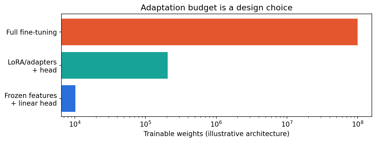
with rank and a scaling constant . Freeze and learn . Trainable weights drop from to . Initialize so the initial update is zero, and randomly so learning can start. After training, can be merged into , so inference costs nothing extra. QLoRA [31] stores the frozen base weights in 4-bit precision and backpropagates through them into LoRA adapters, cutting memory enough to fine-tune very large models on a single GPU.
Code: a low-rank update with a frozen base
This standalone example trains one adapter step on synthetic input. It shows the parameterization and initial behavior; it does not reproduce a full pretrained-model fine-tuning pipeline.
Code · Python · 24 lines
import torch
from torch import nn
from torch.nn import functional as F

torch.manual_seed(0)
class LoRALinear(nn.Module):
    def __init__(self, din, dout, rank=4, alpha=4):
        super().__init__()
        self.base = nn.Linear(din, dout, bias=False)
        self.base.weight.requires_grad_(False)
        self.A = nn.Parameter(torch.randn(rank, din) * .02)
        self.B = nn.Parameter(torch.zeros(dout, rank))
        self.scale = alpha/rank
    def forward(self, x):
        return self.base(x) + self.scale * F.linear(F.linear(x, self.A), self.B)

layer = LoRALinear(32, 16)
x = torch.randn(8, 32)
assert torch.allclose(layer(x), layer.base(x))
opt = torch.optim.Adam([layer.A, layer.B], lr=.01)
loss = F.mse_loss(layer(x), torch.randn(8, 16))
opt.zero_grad(); loss.backward(); opt.step()
assert layer.base.weight.grad is None
print("trainable:", sum(p.numel() for p in layer.parameters() if p.requires_grad))
It prints trainable: 192, which is , against 512 for the full matrix. The first assertion checks that the zero-initialized leaves the model unchanged at the start; the second, that the frozen base receives no gradient.
LoRA is a parameterization, not a guarantee against overfitting or forgetting. Adapters still require domain validation. Frozen BatchNorm statistics, image normalization, output-label mapping and checkpoint-specific preprocessing also need deliberate treatment.
Prompting and in-context learning
The cheapest adaptation changes no weights: write a better text prompt for CLIP, give SAM a box, or put a few solved examples into a multimodal model’s context, as Flamingo did [27]. The vision–language survey by Zhang et al. [41] compares prompting, feature adaptation and fine-tuning across vision tasks. Prompting is fast to iterate but brittle: small wording changes can move results, so fix and report the prompt protocol.
Video, geometry and world models
Plain version. Beyond recognizing a frame, a model may predict change over time, infer three-dimensional structure, or support action planning.
V-JEPA 2 [11] studies self-supervised video models that predict in feature space rather than pixel space, with an action-conditioned extension used for planning. VGGT [12] predicts camera parameters, depth, point maps and tracks from one or many views in a single feed-forward pass. These illustrate two routes beyond classification: temporal state modeling and geometric inference.
A generated video that looks convincing need not obey physical constraints. A scene reconstruction can be useful without generating photorealistic pixels. Measure multi-view consistency, geometry, action-conditioned outcomes and temporal behavior according to the claimed capability. DLCV 13 · World Models develops partial observability, learned dynamics and planning in more detail.
Risks and evaluation
Plain version. Broad pretraining can carry data biases, unsupported predictions and test-set overlap into evaluation. Check these separately from aggregate benchmark performance.
Data provenance, bias and privacy
Web-scale image–text datasets are too large to inspect by hand. LAION-5B [34] made such a dataset public (5.85 billion CLIP-filtered pairs) and thereby enabled open replication such as OpenCLIP [20]; audits of its predecessor LAION-400M by Birhane et al. [35] documented explicit and stereotyping content in image–text pairs. Downstream systems inherit these associations. Licenses and consent also matter: training data, model weights and generated outputs may each carry different terms, and personal data (faces, names, medical images) raises privacy obligations that do not disappear because data was public. SAM’s SA-1B is an example of a dataset whose description emphasizes licensed and privacy-respecting images [5]; record such properties for every model you deploy.
Hallucination
Multimodal LLMs can mention objects that are absent from the image. POPE [37] measures object hallucination with a polling approach: it asks yes/no questions about the presence of specific objects (including frequent and co-occurring distractors), which makes the measurement less dependent on the model’s generation style than scoring free-form captions. A low POPE error does not cover counting, attributes or relations; test those separately.
Contamination and “zero-shot”
If benchmark images (or near-duplicates) are in the pretraining set, a “zero-shot” score partly measures memory. Mayilvahanan et al. [36] asked whether CLIP’s generalization mainly stems from high train–test similarity; after pruning LAION to remove images too similar to common out-of-distribution benchmarks and retraining, performance dropped on some benchmarks but remained strong overall. The lesson is two-sided: similarity explains part of the reported performance, not all of it — so measure it rather than assume either way. Practical checks: deduplicate the test set against available training data, report results on data collected after the model’s data cutoff, and state the full zero-shot protocol (class names, templates, candidate set).
Benchmarks
Aggregate multimodal benchmarks such as MMMU [38] — 11.5K college-level questions from exams, quizzes and textbooks across six disciplines, with charts, diagrams, maps, tables and other image types — test knowledge and reasoning, but a single number mixes perception, OCR, domain knowledge and answer formatting. For a deployment, build a small, task-specific evaluation set with known failure cases, report variance over seeds or prompt wordings, and compare against a simple baseline (a linear probe on frozen features is often surprisingly strong). ML 11 · Evaluation and Deployment covers calibration, splits and deployment in depth.
Modern view
Surveys worth reading.
- Bommasani et al. [1] — the report that named foundation models. It covers capabilities (language, vision, robotics, reasoning), applications (law, health, education), technology (modeling, training, adaptation, evaluation, data) and societal impact. Its key takeaways — emergence, homogenization, and inherited failure — still frame the field.
- Awais et al. [39] — a computer-vision survey organizing foundation models by architecture design, training objective (contrastive versus generative), datasets, fine-tuning mechanisms and prompting, and listing open challenges in evaluation, real-world applicability, adversarial robustness and interpretability.
- Zhang et al. [41] — a TPAMI survey of vision–language models for vision tasks: network architectures, pre-training objectives, downstream tasks, datasets, transfer learning and knowledge distillation, with benchmarking of reviewed methods.
- Yin et al. [40] and Caffagni et al. [2] — surveys of multimodal large language models: architecture (encoder, connector, LLM), training strategy and data (pre-training, instruction tuning, alignment), evaluation, and hallucination.
- Han et al. [13] — a survey broadening the map to multimodal generative models, organized by generative category and technique.
- Xu et al. [42] — a critical review of parameter-efficient fine-tuning that sorts methods into additive, partial, reparameterized, hybrid and unified families and compares representative ones experimentally.
State of the art, 2023–2026. Four trends stand out. (1) Better frozen features: DINOv2 [15] and DINOv3 [16] made self-supervised encoders strong enough that many dense tasks start from frozen patch features. (2) Concept-level prompting: segmentation moved from “click an object” (SAM [5]) to video memory (SAM 2 [6]) to “segment every instance of this phrase” (SAM 3 [7]). (3) Long, interleaved multimodal contexts: models such as Qwen3-VL [9] read many images, video and text together. (4) Beyond recognition: video prediction for planning (V-JEPA 2 [11]) and feed-forward geometry (VGGT [12]) treat foundation models as world and scene estimators.
Open problems.
- Grounded reliability: reducing hallucination and making models say “not visible” when appropriate [37].
- Honest evaluation under contamination and benchmark saturation [36].
- Data: curation as a scaling axis [15], [20], provenance, licensing and consent [34], [35].
- Efficient adaptation and inference: token budgets for high-resolution images and video; PEFT that preserves robustness [32], [33].
- Dense, 3D and temporal understanding that matches the semantic strength of image-level models.
For any new “foundation” model, record its input/output interface, training objective, data sources, supported adaptation, checkpoint license, preprocessing and task-level evaluation. This avoids treating model size or an open-ended chat interface as proof of general competence.
Key takeaways
- Foundation models combine broad pretraining with reuse; the term does not specify one architecture or require text generation.
- Scaling laws are empirical fits tied to data, objectives and training recipes; extrapolation requires validation.
- Pretraining objectives shape capabilities but do not uniquely determine downstream performance.
- Image–text similarity supports retrieval and text-defined classes; similarity is not calibrated confidence.
- Visual prompts and connectors control information access; report prompt construction and image-resolution constraints.
- Start with inexpensive adaptation baselines, then test stronger methods for gains, cost, shift sensitivity, hallucination and contamination.
Exercises
- Candidate dependence. Add a fourth description to the synthetic CLIP example. Can the softmax “confidence” for an image change without changing the image?
Hint
Yes: the denominator of the softmax changes. Similarity to a fixed description is unchanged, but the normalized probability depends on the candidate set. Try adding a text vector close to the ambiguous image’s embedding.
- Compute-optimal allocation. Using the parametric law and , show that the optimal model size grows as . What does imply?
Hint
Substitute , differentiate with respect to and set to zero: . Solving gives . With , and therefore too: scale parameters and tokens equally, as Hoffmann et al. concluded.
- Break the transfer. In the linear-probe experiment, make the downstream class depend on the nuisance factors instead of the semantic ones. What happens to the frozen-feature probe as labels increase, and what does that say about choosing a foundation model?
Hint
Draw class centers for u instead of z. The frozen 8-D features were trained to discard the nuisance directions, so they stay near chance however many labels you add, while the raw-input probe improves. A backbone is only useful if its pretraining kept the information your task needs — check with a linear probe before investing in adaptation.
- LoRA budget. A ViT-B block has four attention projections and two MLP matrices of sizes and . Count trainable weights for full fine-tuning of these six matrices and for rank-8 LoRA on all of them.
Hint
Full: . LoRA: , about 1.6% of the full count.
- Prompt fairness. Design a SAM evaluation that separates mask quality from prompt quality.
Hint
Fix the prompt protocol and count human interactions. Evaluate automatic proposals separately from masks produced with ideal ground-truth prompts, and report both. For SAM 3, compare noun-phrase prompts with exemplar prompts on the same images.
- Contamination audit. You are given a new image–text model that reports high zero-shot accuracy on a public benchmark. List three checks you would run before trusting the number.
Hint
(a) Near-duplicate search of test images against any available training data (e.g. by embedding similarity); (b) evaluation on a freshly collected set from after the data cutoff; (c) sensitivity to the prompt templates and the candidate class list; optionally compare with a linear probe and a simple baseline.
References
- R. Bommasani et al., “On the Opportunities and Risks of Foundation Models,” Stanford CRFM report, arXiv:2108.07258, 2021; revised 2022. arXiv
- D. Caffagni et al., “The Revolution of Multimodal Large Language Models: A Survey,” Findings of ACL, 2024. arXiv
- A. Radford et al., “Learning Transferable Visual Models From Natural Language Supervision,” ICML, 2021. arXiv
- X. Zhai, B. Mustafa, A. Kolesnikov and L. Beyer, “Sigmoid Loss for Language Image Pre-Training,” ICCV, 2023. arXiv
- A. Kirillov et al., “Segment Anything,” ICCV, 2023. arXiv
- N. Ravi et al., “SAM 2: Segment Anything in Images and Videos,” ICLR, 2025. arXiv
- N. Carion et al., “SAM 3: Segment Anything with Concepts,” arXiv:2511.16719, 2025; revised March 2026. arXiv
- H. Liu, C. Li, Q. Wu and Y. J. Lee, “Visual Instruction Tuning,” NeurIPS, 2023. arXiv
- S. Bai et al., “Qwen3-VL Technical Report,” arXiv:2511.21631, 2025. arXiv
- E. J. Hu et al., “LoRA: Low-Rank Adaptation of Large Language Models,” ICLR, 2022. arXiv
- M. Assran et al., “V-JEPA 2: Self-Supervised Video Models Enable Understanding, Prediction and Planning,” arXiv:2506.09985, 2025. arXiv
- J. Wang et al., “VGGT: Visual Geometry Grounded Transformer,” CVPR, 2025. arXiv
- L. Han et al., “A Survey of Generative Categories and Techniques in Multimodal Generative Models,” arXiv:2506.10016, 2025. arXiv
- C. M. Bishop and H. Bishop, Deep Learning: Foundations and Concepts, Springer, 2024. Book
- M. Oquab et al., “DINOv2: Learning Robust Visual Features without Supervision,” Transactions on Machine Learning Research, 2024. arXiv
- O. Siméoni et al., “DINOv3,” arXiv:2508.10104, 2025. arXiv
- J. Kaplan et al., “Scaling Laws for Neural Language Models,” arXiv:2001.08361, 2020. arXiv
- J. Hoffmann et al., “Training Compute-Optimal Large Language Models,” arXiv:2203.15556, 2022; published as “An empirical analysis of compute-optimal large language model training,” NeurIPS, 2022. arXiv
- X. Zhai, A. Kolesnikov, N. Houlsby and L. Beyer, “Scaling Vision Transformers,” CVPR, 2022. arXiv
- M. Cherti et al., “Reproducible Scaling Laws for Contrastive Language-Image Learning,” CVPR, 2023. arXiv
- A. Dosovitskiy et al., “An Image is Worth 16x16 Words: Transformers for Image Recognition at Scale,” ICLR, 2021. arXiv
- K. He, X. Chen, S. Xie, Y. Li, P. Dollár and R. Girshick, “Masked Autoencoders Are Scalable Vision Learners,” CVPR, 2022. arXiv
- H. Bao, L. Dong, S. Piao and F. Wei, “BEiT: BERT Pre-Training of Image Transformers,” ICLR, 2022. arXiv
- M. Caron et al., “Emerging Properties in Self-Supervised Vision Transformers,” ICCV, 2021. arXiv
- C. Jia et al., “Scaling Up Visual and Vision-Language Representation Learning With Noisy Text Supervision,” ICML, 2021. arXiv
- J. Li, D. Li, S. Savarese and S. Hoi, “BLIP-2: Bootstrapping Language-Image Pre-training with Frozen Image Encoders and Large Language Models,” ICML, 2023. PMLR
- J.-B. Alayrac et al., “Flamingo: a Visual Language Model for Few-Shot Learning,” NeurIPS, 2022. arXiv
- H. Liu, C. Li, Y. Li and Y. J. Lee, “Improved Baselines with Visual Instruction Tuning,” CVPR, 2024. arXiv
- N. Houlsby et al., “Parameter-Efficient Transfer Learning for NLP,” ICML, 2019. PMLR
- M. Jia et al., “Visual Prompt Tuning,” ECCV, 2022. arXiv
- T. Dettmers, A. Pagnoni, A. Holtzman and L. Zettlemoyer, “QLoRA: Efficient Finetuning of Quantized LLMs,” NeurIPS, 2023. arXiv
- A. Kumar, A. Raghunathan, R. Jones, T. Ma and P. Liang, “Fine-Tuning can Distort Pretrained Features and Underperform Out-of-Distribution,” ICLR, 2022. arXiv
- M. Wortsman et al., “Robust Fine-Tuning of Zero-Shot Models,” CVPR, 2022. arXiv
- C. Schuhmann et al., “LAION-5B: An Open Large-Scale Dataset for Training Next Generation Image-Text Models,” NeurIPS Datasets and Benchmarks Track, 2022. arXiv
- A. Birhane, V. U. Prabhu and E. Kahembwe, “Multimodal Datasets: Misogyny, Pornography, and Malignant Stereotypes,” arXiv:2110.01963, 2021. arXiv
- P. Mayilvahanan, T. Wiedemer, E. Rusak, M. Bethge and W. Brendel, “Does CLIP’s Generalization Performance Mainly Stem from High Train-Test Similarity?,” ICLR, 2024. arXiv
- Y. Li et al., “Evaluating Object Hallucination in Large Vision-Language Models,” EMNLP, 2023. arXiv
- X. Yue et al., “MMMU: A Massive Multi-discipline Multimodal Understanding and Reasoning Benchmark for Expert AGI,” CVPR, 2024. arXiv
- M. Awais et al., “Foundational Models Defining a New Era in Vision: A Survey and Outlook,” arXiv:2307.13721, 2023. arXiv
- S. Yin et al., “A Survey on Multimodal Large Language Models,” National Science Review, 2024. arXiv
- J. Zhang, J. Huang, S. Jin and S. Lu, “Vision-Language Models for Vision Tasks: A Survey,” IEEE TPAMI, vol. 46, no. 8, 2024. arXiv
- L. Xu et al., “Parameter-Efficient Fine-Tuning Methods for Pretrained Language Models: A Critical Review and Assessment,” arXiv:2312.12148, 2023. arXiv
- J. Deng, W. Dong, R. Socher, L.-J. Li, K. Li and L. Fei-Fei, “ImageNet: A Large-Scale Hierarchical Image Database,” CVPR, 2009, pp. 248–255. doi
- J. Devlin, M.-W. Chang, K. Lee and K. Toutanova, “BERT: Pre-training of Deep Bidirectional Transformers for Language Understanding,” NAACL-HLT, 2019, pp. 4171–4186. doi
- OpenAI, “GPT-4 Technical Report,” arXiv:2303.08774, 2023. arXiv
Check your understanding
This tutorial has 6 exercises. Can you solve them without opening the hints?
Go to the exercises ↑Next ML 11 · Evaluation, Efficiency and Deployment · 30 min