ML 06 · Representation Learning and Self-Supervision
Needs: ML 05 · Attention and Vision Transformers
Navigate: this page and this track: Navigate: this page and this track
On this page
- What you’ll learn1 min
- The big picture1 min
- What is a representation?3 min
- Transfer learning: pretrain once, reuse many times1 min
- Self-supervised learning: let the data make the labels1 min
- Contrastive learning and the InfoNCE loss5 min
- A worked example: SimCLR on 8×8 digits1 min
- Without negatives: why matching alone can collapse3 min
- Masked modeling: learn by filling gaps2 min
- Language as supervision: CLIP1 min
- DINOv2 and DINOv3: features as a product1 min
- Evaluate transfer honestly2 min
- Modern view2 min
- Key takeaways1 min
- Exercises2 min
- Paper guides
- References
Machine Learning
Explore this chapter 1 interactive experiment
Move paired and unpaired unit vectors, then inspect the normalized matching loss used by contrastive learning.
What you’ll learn
- Define useful representations and task-dependent invariances.
- Reuse features through nearest neighbors, linear probes or fine-tuning.
- Compare contrastive, teacher–student, masked and feature-prediction objectives.
- Explain representation collapse and mechanisms that discourage it.
- Evaluate transfer and image–text alignment under explicit protocols.
The big picture
Suppose you have a million unlabeled images but only 500 labeled examples for the task you care about. Training a large network from scratch on those 500 examples ignores almost all the available data. Representation learning splits the job in two. First, learn an encoder from a broad signal that does not need your labels. Second, train a small task-specific head on top of using the few labels you have.
Why it matters: almost every modern vision system starts from a pretrained encoder. Image classifiers, detectors, segmentation models, image–text models and the image encoders inside generative models are built on representations learned this way. The quality of that starting point often matters more than the details of the task head.
This chapter starts with what a representation is and why transfer works, then walks through the self-supervised objectives that dominate practice, and ends with how to measure whether a representation is any good. It assumes you know neural networks (ML 02), CNNs (ML 03) and vision transformers (ML 05). Linear factor models and autoencoders, the classical route to representations, have their own chapter: ML 06A.
What is a representation?
Plain version. A representation is the list of numbers a model uses to describe an input. A good one makes the things you care about easy to read off, and hides the things you do not care about.
Precise version. An encoder is a function from inputs (here, images) to feature vectors , where are the learnable parameters and is the feature dimension. A task head maps to a prediction, so the full model is . We call a good representation for a task when a simple head, such as a linear classifier, can solve the task from using few labeled examples. Bengio, Courville and Vincent’s review [1] is the classic statement of this view; it lists the “priors” that make representations useful, such as smoothness, multiple explanatory factors, a hierarchy of increasingly abstract features, and shared factors across tasks.
Local versus distributed representations
The simplest representation of a category is one-hot: one unit per concept, with exactly one unit on. It is easy to read but it cannot generalize. Knowing about “red car” says nothing about “red truck”, because they share no active units. A distributed representation describes each input with many features that are each shared by many inputs: “red”, “blue”, “car”, “truck”. Now “red truck” reuses the “red” unit learned from red cars.
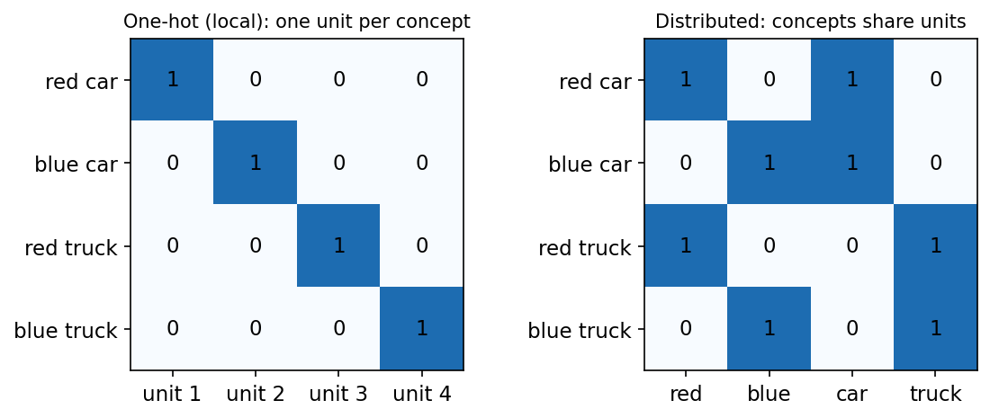
The counting argument is striking. With binary features, a one-hot code distinguishes concepts, while a distributed code can in principle distinguish configurations [1]. Deep networks learn distributed codes automatically: each hidden unit responds to many inputs, and each input activates many units. Most of the practical value of representation learning comes from this sharing.
Invariance and equivariance
A useful representation keeps differences relevant to the task and suppresses differences that distract from it.
- A feature is invariant to a transformation if : shifting a cat by two pixels should not change “this is a cat”.
- A feature is equivariant if it changes in a predictable way, : shifting the cat should shift its segmentation mask by the same amount.
“Useful” always depends on the downstream task. Color invariance helps object recognition but hurts fruit-ripeness estimation. Rotation invariance helps for textures but confuses 6 and 9. Dense prediction (segmentation, depth) needs spatially equivariant patch features, not a single invariant vector per image. We will see that self-supervised objectives choose their invariances mostly through the data augmentations they use, so this choice is a modeling decision, not a detail.
Learning distances: metric learning
PCA, introduced in ML 01 and developed in ML 06A, keeps the directions of highest variance. But high variance may come from lighting rather than object identity. Supervised learning shapes features around labels; metric learning shapes distances around pairs that should match. For an anchor , a positive (same identity) and a negative (different identity), the triplet loss is
where are the three feature vectors and is a margin. The loss is zero once the positive is closer than the negative by at least . An easy negative gives zero loss and teaches nothing, so choosing informative (“hard”) negatives matters. Contrastive self-supervised learning, below, is metric learning in which the positives are created by augmentation instead of by labels.
Transfer learning: pretrain once, reuse many times
Plain version. Train a network on a big task, keep its feature extractor, and reuse it for a small task. You can freeze the features and only train a new head, or let the whole network keep learning.
Precise version. Pretraining finds encoder parameters on a source dataset or objective. Transfer to a target task with labeled set uses one of three protocols:
- -nearest neighbors (-NN): no training. Classify a test feature by the labels of its most similar training features.
- Linear probe: keep frozen and fit a linear classifier on , where and are the only trained parameters.
- Fine-tuning: start from and update the encoder together with the head, usually with a small learning rate.
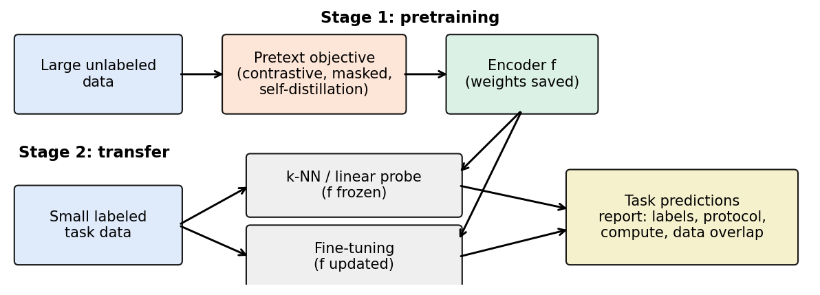
Why does transfer work at all? Yosinski et al. [2] measured it layer by layer on ImageNet-trained CNNs. First-layer features (edge and color detectors much like Gabor filters) were general: they transferred well between tasks. Features became progressively more specific to the source task in higher layers, and transferability decreased as the source and target tasks became more different. They also found that initializing from transferred features and fine-tuning improved generalization even on the target task, compared with training from random initialization.
For years, the default pretraining source was supervised ImageNet classification. Labels are expensive, though, and a label like “dog” tells the network nothing about the dog’s pose, the grass or the lighting. Self-supervised learning removes the label bottleneck by making the data supervise itself.
Self-supervised learning: let the data make the labels
Plain version. Build prediction targets from the data, such as matching two views or recovering masked content. Whether the learned features transfer still needs testing.
Precise version. A self-supervised objective is a loss computed from unlabeled inputs alone (or from naturally paired data such as image–caption pairs). The surveys by Liu et al. [3] and Gui et al. [4] and the practical “cookbook” by Balestriero et al. [5] organize the field into the families summarized here:
| Family | Training signal | Representative methods | Main risk |
|---|---|---|---|
| Contrastive | Pull positive pairs together, push other samples apart | SimCLR, MoCo | Needs many negatives; false negatives |
| Self-distillation (no negatives) | Student matches a teacher on another view | BYOL, SimSiam, DINO | Collapse without asymmetry or centering |
| Redundancy reduction | Agreement plus decorrelated, non-constant feature dimensions | Barlow Twins, VICReg | Extra hyperparameters for the regularizers |
| Masked modeling | Predict hidden pixels or tokens | BEiT, MAE | Features may focus on low-level detail |
| Feature prediction | Predict features of hidden regions | I-JEPA, V-JEPA 2 | Needs anti-collapse design like distillation |
| Language supervision | Match images with their captions | CLIP, SigLIP | Inherits web-data biases and noise |
The families are learning objectives, not architectures: each can train a CNN or a transformer. Modern systems often combine several of them. The sections below take them in turn.
Contrastive learning and the InfoNCE loss
Plain version. Make two augmented versions of the same image agree, and make them disagree with every other image in the batch. It is a multiple-choice question: “out of these candidates, which one is my partner?”
InfoNCE
Van den Oord, Li and Vinyals introduced the InfoNCE loss in Contrastive Predictive Coding (CPC) [6]. Take a query , one positive key that “belongs” to it, and negative keys . With a similarity score and a temperature ,
This is exactly softmax cross-entropy for an -way classification problem whose correct class is the positive. Two consequences follow.
- A lower bound on mutual information. CPC shows that , where is mutual information. Minimizing the loss raises this lower bound, and more negatives (larger ) allow a higher bound. In practice this bound is loose, and the quality of the features depends heavily on the encoder and augmentations, so read it as motivation rather than as the explanation of why the features are good.
- The temperature controls hardness. Dividing by a small sharpens the softmax, so the loss concentrates on the negatives most similar to the query (the hard negatives).
SimCLR
SimCLR [7] is InfoNCE in its simplest form. Take a batch of images and produce two augmented views of each (random crop and resize, color distortion, blur), giving views. A backbone maps each view to , a small MLP projection head maps to , and the similarity is cosine similarity . For view with partner ,
where the are -normalized and the sum runs over all other views. Every other image in the batch is a negative, so no memory bank is needed, but the method benefits from large batches. The total loss averages over both orderings of every positive pair; the paper calls this the NT-Xent loss (normalized temperature-scaled cross-entropy).
Three findings from the SimCLR paper are worth remembering [7]. The composition of augmentations matters a lot, with random cropping plus color distortion being especially important. The projection head helps: features before the head () transfer better than those after it (), so the head is discarded after pretraining. And contrastive learning benefits from larger batches and longer training than supervised learning.
Code: check the loss and its collapse value
This standalone PyTorch example uses synthetic paired vectors to verify the loss, the self-mask and the gradients. It does not train an encoder.
Code · Python · 23 lines
import torch
from torch.nn import functional as F

torch.manual_seed(0)
B, D = 8, 16
base = torch.randn(B, D)
views = torch.cat([base + .1*torch.randn_like(base),
                   base + .1*torch.randn_like(base)]).requires_grad_()
z = F.normalize(views, dim=-1)
logits = z @ z.T / .2
self_mask = torch.eye(2*B, dtype=torch.bool)
logits = logits.masked_fill(self_mask, float("-inf"))
positive = (torch.arange(2*B) + B) % (2*B)
loss = F.cross_entropy(logits, positive)
loss.backward()
assert torch.isfinite(views.grad).all()
print("paired loss:", round(loss.item(), 4))

collapsed = F.normalize(torch.ones(2*B, D), dim=-1)
scores = (collapsed @ collapsed.T / .2).masked_fill(self_mask, float("-inf"))
collapsed_loss = F.cross_entropy(scores, positive)
print("collapsed loss:", round(collapsed_loss.item(), 4))
print("expected:", round(torch.log(torch.tensor(2*B-1.)).item(), 4))
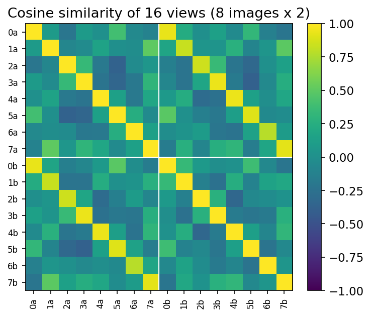
It prints a paired loss of 0.1423 and a collapsed loss of 2.7081, equal to . If every representation is identical, the positive gets probability and the loss is , the worst value a uniform guess can get. Contrastive discrimination therefore makes complete collapse a bad solution, although optimization and negative selection can still be difficult.
MoCo: a queue of negatives and a momentum encoder
InfoNCE prefers many negatives, but SimCLR gets them only from the current batch. Momentum Contrast (MoCo) [8] decouples the number of negatives from the batch size with two ideas.
- A queue. Keys encoded in recent batches are stored in a first-in, first-out queue of length and reused as negatives. The query sees negatives no matter how small the batch is.
- A momentum encoder. Keys in the queue were produced by slightly older networks. If the key encoder changed quickly, old and new keys would be inconsistent. MoCo therefore computes keys with a separate encoder whose parameters follow the query encoder’s parameters slowly:
where is the momentum, close to 1 (the paper’s default is 0.999). Only receives gradients. This exponential moving average (EMA) teacher idea reappears in BYOL, DINO and JEPA.
Code · Python · 21 lines
import torch
from torch.nn import functional as F

torch.manual_seed(0)
B, D, K = 8, 16, 32          # batch, embedding size, queue length

# --- MoCo-style InfoNCE: one positive key per query, negatives from a queue
q = F.normalize(torch.randn(B, D), dim=1)                 # queries (online encoder)
k = F.normalize(q + 0.1 * torch.randn(B, D), dim=1)       # keys (momentum encoder)
queue = F.normalize(torch.randn(K, D), dim=1)             # keys from past batches
l_pos = (q * k).sum(1, keepdim=True)                      # B x 1
l_neg = q @ queue.T                                       # B x K
logits = torch.cat([l_pos, l_neg], dim=1) / 0.07
loss_moco = F.cross_entropy(logits, torch.zeros(B, dtype=torch.long))
queue = torch.cat([k, queue])[:K]                         # enqueue new, drop oldest
print("MoCo logits:", tuple(logits.shape), "loss:", round(loss_moco.item(), 3))

# momentum (EMA) update of the key encoder's parameters
theta_q, theta_k, m = torch.randn(5), torch.zeros(5), 0.999
theta_k = m * theta_k + (1 - m) * theta_q
print("key params moved by:", round((theta_k.norm() / theta_q.norm()).item(), 4))
Each query gets a -way classification problem whose correct answer is always column 0, hence the all-zero targets. The output shows logits of shape (8, 33), and the EMA step moves the key encoder only 0.1% of the way toward the query encoder (from zero, after one step). In a real implementation, and come from the two encoders applied to two augmentations of the same images.
Alignment and uniformity
Wang and Isola [9] gave a clean geometric reading of what contrastive losses do on the unit sphere. With normalized features, the loss asymptotically optimizes two properties:
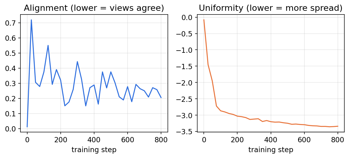
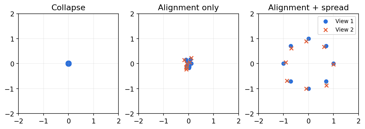
where is a positive pair, are independent samples, and (commonly ). Alignment is low when positive pairs map to nearby points. Uniformity is low when features spread out over the sphere, so they keep as much information about the input as possible. A collapsed encoder has perfect alignment (0) and the worst uniformity (0); a useful encoder has both small.
Code · Python · 18 lines
import torch
from torch.nn import functional as F

def alignment(z1, z2):            # mean squared distance between positive pairs
    return (z1 - z2).square().sum(1).mean()

def uniformity(z, t=2.0):         # log of mean Gaussian potential over all pairs
    return torch.pdist(z).square().mul(-t).exp().mean().log()

torch.manual_seed(0)
n, D = 512, 16
collapsed = F.normalize(torch.ones(n, D), dim=1)
spread = F.normalize(torch.randn(n, D), dim=1)
noisy_view = F.normalize(spread + 0.1 * torch.randn(n, D), dim=1)
print("collapsed: align", alignment(collapsed, collapsed).item(),
      "uniform", round(uniformity(collapsed).item(), 3))
print("spread:    align", round(alignment(spread, noisy_view).item(), 3),
      "uniform", round(uniformity(spread).item(), 3))
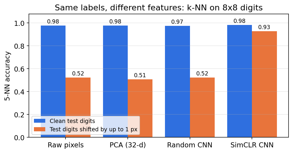
The collapsed set scores alignment 0.0 and uniformity 0.0; the spread set scores about 0.138 and −3.51. Figure 4 tracks the same two quantities while training the digit encoder below. At step 0 the random network maps every view to almost the same point, so alignment is near zero only because everything has collapsed. Training first spreads the features out (uniformity drops sharply), then gradually pulls positives back together.
A worked example: SimCLR on 8×8 digits
Plain version. Train a tiny SimCLR encoder on scikit-learn’s digits without using any labels, then check whether its features make a nearest-neighbor classifier more robust.
The augmentation here is a random shift of up to one pixel, a random brightness change and pixel noise. We therefore expect the learned features to be roughly invariant to small shifts, something raw pixels are not. The evaluation uses the same labeled training set for every feature type and tests on clean digits and on digits shifted by up to one pixel.
Code · Python · 55 lines
import copy
import numpy as np
import torch
from torch import nn
from torch.nn import functional as F
from sklearn.datasets import load_digits
from sklearn.decomposition import PCA
from sklearn.model_selection import train_test_split
from sklearn.neighbors import KNeighborsClassifier

torch.manual_seed(0); np.random.seed(0); torch.set_num_threads(1)
d = load_digits()
Xtr, Xte, ytr, yte = train_test_split(d.data / 16., d.target, test_size=.3,
                                      random_state=0, stratify=d.target)
Xtr_t = torch.tensor(Xtr, dtype=torch.float32)

def augment(x):                      # the augmentations define the invariances
    img = F.pad(x.view(-1, 1, 8, 8), (1, 1, 1, 1))
    i, j = np.random.randint(0, 3, size=2)               # shift by up to 1 px
    img = img[:, :, i:i + 8, j:j + 8]
    img = img * (0.7 + 0.6 * torch.rand(len(img), 1, 1, 1))  # brightness
    return (img + 0.1 * torch.randn_like(img)).reshape(len(x), 64)  # noise

backbone = nn.Sequential(nn.Unflatten(1, (1, 8, 8)),
                         nn.Conv2d(1, 32, 3, padding=1), nn.ReLU(),
                         nn.Conv2d(32, 64, 3, padding=1), nn.ReLU(),
                         nn.AdaptiveAvgPool2d(2), nn.Flatten())  # h: 256-d
random_backbone = copy.deepcopy(backbone)                    # baseline
head = nn.Sequential(nn.ReLU(), nn.Linear(256, 64))          # projection g
opt = torch.optim.Adam([*backbone.parameters(), *head.parameters()], lr=1e-3)

def nt_xent(z1, z2, tau=0.2):
    z = F.normalize(torch.cat([z1, z2]), dim=-1)
    n = len(z1)
    logits = (z @ z.T / tau).fill_diagonal_(float("-inf"))
    return F.cross_entropy(logits, (torch.arange(2 * n) + n) % (2 * n))

for step in range(800):                                 # about a minute on CPU
    x = Xtr_t[torch.randint(len(Xtr_t), (256,))]
    loss = nt_xent(head(backbone(augment(x))), head(backbone(augment(x))))
    opt.zero_grad(); loss.backward(); opt.step()

def shift(x, dy, dx):                   # move one 8x8 image, fill with zeros
    img = np.zeros((10, 10)); img[1:9, 1:9] = x.reshape(8, 8)
    return img[1 - dy:9 - dy, 1 - dx:9 - dx].ravel()

moves = np.random.default_rng(0).integers(-1, 2, size=(len(Xte), 2))
Xte_shift = np.stack([shift(x, *m) for x, m in zip(Xte, moves)])
enc = lambda net: (lambda A: net(torch.tensor(A, dtype=torch.float32)).detach().numpy())
pca = PCA(32, random_state=0).fit(Xtr)
for name, f in [("raw pixels", lambda A: A), ("PCA-32", pca.transform),
                ("random CNN", enc(random_backbone)), ("SimCLR CNN", enc(backbone))]:
    knn = KNeighborsClassifier(5, metric="cosine").fit(f(Xtr), ytr)
    print(f"{name:11s} clean {knn.score(f(Xte), yte):.3f}  "
          f"shifted {knn.score(f(Xte_shift), yte):.3f}")
On our machine this prints:
Code · 4 lines
raw pixels  clean 0.978  shifted 0.524
PCA-32      clean 0.978  shifted 0.507
random CNN  clean 0.974  shifted 0.524
SimCLR CNN  clean 0.987  shifted 0.919
Exact numbers vary slightly across PyTorch versions and hardware. The pattern is the lesson. On clean digits, raw pixels are already excellent: this dataset is easy, and a fancy encoder adds little. On shifted digits, raw pixels, PCA and an untrained CNN of the same architecture all drop to about 50%, while the self-supervised features keep most of their accuracy. The network learned the invariance we asked for through the augmentations, and nothing more: had we tested on rotated digits, which the augmentations never showed, we should not expect the same robustness.
Optional: SimCLR (in the Paper guides). Read the original figure, evidence, design choices and limitations.
Without negatives: why matching alone can collapse
Plain version. If the only instruction is “make the two outputs agree”, returning the same constant for every image solves it perfectly. Methods without negatives need some other mechanism to stop this.
Minimizing over two views has the trivial solution for a constant . Agreement alone does not require the features to carry any information. Complete collapse maps everything to one point; dimensional collapse is subtler: the features vary, but only along a few directions, wasting most of the dimensions.
BYOL: an online network chases a slow target
BYOL [10] uses two networks. The online network (encoder, projector and an extra predictor ) is trained to predict the target network’s projection of a different view of the same image. The target is not trained by gradients; it is an EMA of the online weights, as in MoCo:
The loss is the squared distance between the normalized prediction and the normalized target projection, symmetrized over the two views. The target output is treated as a constant (stop-gradient). There are no negatives, yet BYOL does not collapse in practice. The asymmetry (predictor on one side, stop-gradient and EMA on the other) and the full training recipe matter; EMA alone does not prove collapse impossible.
SimSiam: stop-gradient is the key ingredient
Chen and He’s SimSiam [11] stripped BYOL down further: one shared encoder for both views, a predictor on one branch, no momentum encoder, no negatives and no large batches. With and ,
where is stop-gradient and is negative cosine similarity. The paper’s experiments show that removing the stop-gradient makes the model collapse quickly, while the predictor is also needed. The authors interpret the method as an alternating, expectation-maximization-like optimization. The practical lesson: very small architectural asymmetries decide whether these methods learn or collapse.
DINO: self-distillation with centering and sharpening
DINO [12] turns the agreement problem into classification with soft labels. Teacher and student both output a probability vector over “prototype” dimensions via a temperature-scaled softmax. The student, seeing a view , is trained to match the teacher’s distribution on another view :
where is the teacher network (an EMA of the student), is a running mean of teacher outputs (centering) and is a low teacher temperature (sharpening). Centering stops one dimension from dominating; sharpening stops the output from becoming uniform. Each alone collapses in a different way; together they balance. DINO also uses multi-crop: the teacher sees only large global crops, while the student also sees small local crops, so the student must infer global content from local evidence. With vision transformers, DINO’s attention maps were notable for highlighting object boundaries without any segmentation labels.
Barlow Twins and VICReg: regularize the statistics directly
A different route is to forbid collapse explicitly in the loss. Barlow Twins [13] computes the cross-correlation matrix between the (batch-standardized) embeddings of the two views and pushes it toward the identity:
where the first term makes each dimension agree across views and the second, weighted by , decorrelates different dimensions so they do not carry redundant information. VICReg [14] splits the same idea into three named terms: invariance (mean squared distance between the two embeddings), variance (a hinge loss keeping the standard deviation of every dimension above a threshold, which directly forbids constant outputs) and covariance (penalizing off-diagonal covariance entries). “No negatives” does not mean “no anti-collapse design”; these methods simply put the design in the loss instead of in the architecture.
Masked modeling: learn by filling gaps
Plain version. Hide part of the input and predict what is missing. This is how BERT learned language, and it works for images too, once you choose the right amount of hiding.
BEiT [15] brought BERT-style pretraining to vision transformers. An image is split into patches; some are masked, and the network predicts discrete visual tokens for the masked positions, where the tokens come from a separately trained image tokenizer.
MAE [16] predicts raw pixels instead. It masks a large fraction of the patches, sends only the visible ones through the encoder, and reconstructs the missing pixels with a lightweight decoder. With the set of masked patch indices ,
where is the true pixel vector of patch and is the prediction. MAE’s design choices are deliberate. A high masking ratio (75% by default) makes the task hard enough that the network cannot simply interpolate from neighbors. The encoder only processes visible patches, which cuts pretraining cost. Normalizing each target patch by its own mean and variance improves the features. After pretraining, the decoder is discarded.
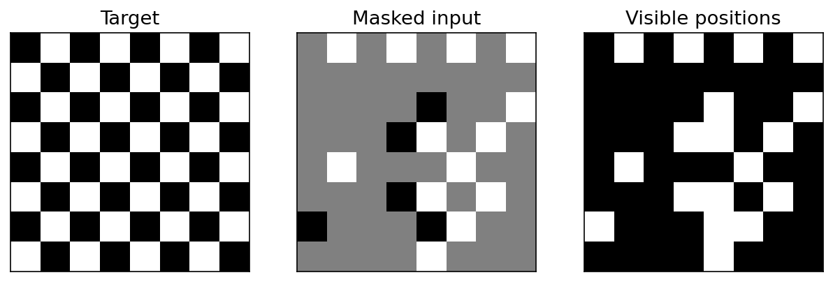
Reconstruction is not the same as generation. A model that predicts masked pixels from visible ones is not trained to sample complete images from scratch. Low reconstruction loss does not guarantee the best semantic features either: background texture can dominate pixel error. Masked-modeling features are typically weaker than contrastive or distillation features under a linear probe but strong after fine-tuning, which is one reason the evaluation protocol must be stated.
Predicting features instead of pixels: JEPA
Plain version. Instead of painting in every uncertain pixel, predict a description of the hidden region.
I-JEPA [17] (Image Joint-Embedding Predictive Architecture) encodes a visible context block and predicts the encoder features of several target blocks from it. The target encoder is an EMA of the context encoder, and a predictor receives the context features plus the positions of the targets. A simplified objective is
where is the context encoder, the EMA target encoder, the predictor and stop-gradient. The formula summarizes the idea; the masking strategy (large, semantic-scale target blocks) and the architecture are part of the method, not optional details.
V-JEPA 2 [18] extends feature prediction to video at scale. Its report separates action-free pretraining on video from an action-conditioned model, trained afterward on a small amount of robot data, that is used for planning. Predicting future latent states, recognizing actions and generating photorealistic frames are different capabilities, and a “world model” claim should say which one it makes.
Language as supervision: CLIP
Plain version. Align image and caption embeddings, then compare an image with text descriptions of candidate classes. Prompt wording affects the result.
CLIP [19] trains on image–text pairs collected from the web. In a batch of pairs, the image encoder gives normalized embeddings and the text encoder gives . The similarity matrix , with a learned temperature , has the correct pairs on its diagonal. The loss is the average of two InfoNCE losses, one over rows (which caption fits this image?) and one over columns (which image fits this caption?):
Zero-shot classification follows directly. Embed one prompt per class, such as “a photo of a dog”, and assign an image to the class whose prompt embedding is most similar. No task-specific labels are needed, although prompt wording affects accuracy.
SigLIP [20] replaces the softmax with an independent sigmoid loss on every image–text pair: each entry of the matrix becomes a yes/no question, “do these match?”. This removes the need to normalize over the whole batch, which simplifies large-scale distributed training.
Code · Python · 26 lines
import torch
from torch.nn import functional as F

torch.manual_seed(0)
D = 16

# --- CLIP-style symmetric loss on N matched image-text pairs
N = 6
img = F.normalize(torch.randn(N, D), dim=1)
txt = F.normalize(img + 0.3 * torch.randn(N, D), dim=1)   # caption i matches image i
logit_scale = torch.tensor(1 / 0.07)
sim = logit_scale * img @ txt.T                           # N x N, diagonal = matches
labels = torch.arange(N)
loss_clip = (F.cross_entropy(sim, labels) + F.cross_entropy(sim.T, labels)) / 2
print("CLIP loss:", round(loss_clip.item(), 3))

# zero-shot classification: embed one prompt per class, pick the most similar
class_prompts = txt[:3]                                   # stand-ins for "a photo of a {class}"
pred = (img @ class_prompts.T).argmax(1)
print("zero-shot predictions for images 0-2:", pred[:3].tolist())

# SigLIP-style alternative: an independent yes/no decision for every pair
t, b = 10.0, -10.0                                        # learnable in practice
signs = 2 * torch.eye(N) - 1                              # +1 on matches, -1 elsewhere
loss_sig = -F.logsigmoid(signs * (t * img @ txt.T + b)).sum() / N
print("sigmoid loss:", round(loss_sig.item(), 3))
The synthetic captions are noisy copies of the image embeddings, so the CLIP loss is small (0.054) and the zero-shot step recovers the right “classes” [0, 1, 2]. In real CLIP the two encoders are a vision transformer or CNN and a text transformer, and the hard part is the data: what the captions describe, and what they leave out, determines what the representation knows. The sigmoid loss value (3.473) is not comparable to the softmax loss; it uses different units and a bias term .
DINOv2 and DINOv3: features as a product
Plain version. With enough curated data and compute, pretraining can produce an encoder that you freeze and reuse for many different tasks, from classification to depth estimation.
DINOv2 [21] combines image-level self-distillation (as in DINO) with a patch-level masked objective, and pays close attention to data curation: building a large, diverse, deduplicated pretraining set from uncurated images by retrieval against curated ones. The result is a family of frozen encoders whose global and patch features work well with simple heads. DINOv3 [22], released in 2025, scales this further and adds Gram anchoring to counter the degradation of dense (patch) features during long training. Rather than only matching each feature independently, Gram anchoring constrains the matrix of similarities among patch features toward that of an earlier model. The report also distills a very large teacher into smaller models for deployment.
The practical question is whether frozen global or dense features solve your task. A model strong at semantic retrieval may miss a small scratch on a manufactured part. Increasing the input resolution and using patch features can help, but it changes the compute budget and the comparison protocol.
Evaluate transfer honestly
Plain version. Test features on held-out tasks or data with a stated adaptation protocol. Keep evaluation separate from feature and hyperparameter selection.
| Protocol | What is trained | What it measures |
|---|---|---|
| -NN | Nothing; similarity to labeled reference features | Local structure of the representation |
| Linear probe | Linear head; encoder frozen | Information accessible through a simple readout |
| Fine-tuning | Head plus some or all encoder layers | Adaptability under a stated label and compute budget |
| Dense transfer | Spatial head on patch maps | Suitability for pixel or region outputs |
Linear probing versus fine-tuning
Fine-tuning has more freedom, so it usually wins when the target data is plentiful and similar to the pretraining data. It is not always better. Kumar et al. [23] showed theoretically and empirically that full fine-tuning can distort good pretrained features: while a randomly initialized head is still wrong, its large gradients flow into the encoder and change features in directions that suit the training distribution but hurt out-of-distribution (OOD) inputs. A linear probe cannot distort the features. Their remedy, LP-FT, is two-step: first train the linear head with the encoder frozen, then fine-tune everything starting from that head.
We reproduced the qualitative effect on the digits example. The encoder is the SimCLR CNN from above; the labeled training digits are clean; the test digits are shifted, a mild distribution shift. For each label budget, we average three random draws of the labeled examples.
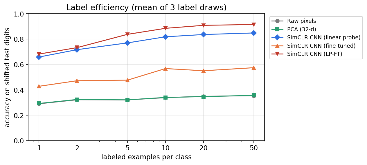
Read Figure 8 for its shape, not its exact values. The frozen SSL features with a linear head need only a handful of labels per class to beat raw pixels with 50 labels per class. Plain fine-tuning with a randomly initialized head did worse than the frozen probe here, and LP-FT did better than both, the same ordering Kumar et al. report under distribution shift. Fine-tuning needs its own hyperparameter search, and the head initialization matters.
Rules against leakage
- Normalize features consistently for similarity comparisons (cosine -NN needs normalized vectors).
- Fit scalers, PCA and classifier hyperparameters on training and validation data only.
- A frozen encoder still has a training history: overlap between pretraining data and evaluation data can inflate results, especially for web-scale models.
- Report the number of labels, backbone, checkpoint, input resolution, augmentations, head, tuning budget and protocol. Choosing the best of many encoders on the test set is test leakage, even if none of them is fine-tuned.
Modern view
Surveys and review papers. Four reviews map the field from complementary angles.
- Bengio, Courville and Vincent (TPAMI 2013) [1] frame the whole enterprise. They ask what makes one representation better than another and answer with a list of generic priors: distributed codes, depth and abstraction, disentangling of explanatory factors, manifolds and natural clustering. They review probabilistic models, autoencoders and manifold learning. It predates modern SSL but remains the best statement of why we learn representations.
- Liu et al. (TKDE 2023) [3] classify self-supervised methods into generative (autoencoding and autoregressive reconstruction), contrastive (context–instance and instance–instance) and generative-contrastive (adversarial) groups across vision, language and graphs, and discuss why contrastive objectives were winning on vision benchmarks at the time.
- Gui et al. (TPAMI 2024) [4] survey algorithms more recently, covering contrastive, self-distillation, redundancy-reduction and masked image modeling methods, and discuss applications and open problems such as theory, the choice of pretext task and multimodal SSL.
- Balestriero et al. (2023) [5] is a practitioner’s guide written by many of the field’s authors. It groups methods into a deep-metric-learning family (SimCLR and relatives), a self-distillation family (BYOL, SimSiam, DINO), a canonical-correlation-analysis family (VICReg, Barlow Twins) and masked image modeling, and collects the “tricks” (augmentations, projectors, EMA schedules, batch-size effects) that the papers often bury. Prince’s textbook [24] gives a gentle, figure-rich introduction to the same ideas with notebooks.
State of practice (2023–2026). The trends visible in the papers cited above are:
- Combined objectives. Leading image encoders mix image-level distillation with patch-level masked prediction (DINOv2 [21], DINOv3 [22]) rather than relying on one pretext task.
- Data as a first-class design choice. DINOv2’s curation pipeline and the web-scale pair collection behind CLIP [19] and SigLIP [20] show that what goes into pretraining matters as much as the loss.
- Dense features. Segmentation, depth and correspondence need good patch features, which motivated objectives like Gram anchoring [22].
- Prediction in latent space and video. I-JEPA [17] and V-JEPA 2 [18] predict features instead of pixels, and extend to video and action-conditioned prediction.
- Language-aligned encoders as the default backbone for multimodal models (see ML 10).
Open problems. We still lack a predictive theory of which pretext task suits which downstream task; collapse is prevented by recipes more than by guarantees; evaluation depends heavily on protocol and on overlap between pretraining and test data; and web-scale pretraining inherits biases and gaps from its data. Our reading of [3], [4], [5], [21], [22] is that data and target design deserve as much attention as architecture. That is an interpretation of the literature, not a theorem that one objective wins everywhere.
The next chapters change the question: instead of describing an image, how can a model describe and sample its whole distribution? See ML 06A for autoencoders and ML 07 for generative models.
Key takeaways
- Useful features make the target task easier; distributed codes alone do not guarantee generalization.
- Augmentations choose which differences to ignore; preserve differences needed by the downstream task.
- Contrastive objectives distinguish positive matches from alternatives; agreement alone admits constant-output collapse.
- Teacher asymmetry, variance constraints and redundancy penalties address collapse in different ways.
- Reconstructing pixels, predicting features and aligning captions train different capabilities.
- Nearest-neighbor tests, linear probes and fine-tuning answer different questions; evaluate adaptation under the expected distribution shift.
Exercises
- Temperature and collapse. In the first code block, change the temperature from 0.2 to 0.05 and to 1.0. Does the collapsed loss change? Does the paired loss?
Hint
The collapsed loss stays : all non-self logits are equal, so dividing them by any leaves the softmax uniform. The paired loss changes, because temperature rescales the differences between scores, and with real differences a smaller gives a sharper softmax.
- Augmentations are assumptions. You want features for (a) counting cells in microscopy, (b) recognizing bird species, (c) reading street-sign text. For each, name one standard SimCLR augmentation you would remove and why.
Hint
(a) Random cropping can change the number of cells in view, so the “same” label is no longer the same. (b) Strong color jitter can remove plumage color, a key species cue. (c) Horizontal flips turn text into mirror text. Decide what must be preserved before choosing invariances.
- MAE compute. An image has 196 patches and MAE masks 75%. How many patches enter the encoder? By what factor does the number of pairwise attention scores in the encoder shrink?
Hint
49 visible patches enter the encoder. Attention scores scale with the square of the token count: . The decoder still processes all 196 positions, but it is small.
- Break the digits experiment. Modify the SimCLR digits code so that
augmentonly adds noise (no shift). Retrain and compare the shifted-test -NN accuracy with the original. What does this tell you?
Hint
Replace the random i, j with i, j = 1, 1. On our machine the shifted-test accuracy fell from 0.919 to 0.743, while clean accuracy stayed at 0.981. Without the shift augmentation, nothing in the objective asks for shift invariance; the robustness that remains comes from what a trained convolution-and-pooling encoder learns anyway (the untrained one in the main example had none). The augmentations, not the word “self-supervised”, decide most of what is learned.
- SimSiam ablation, on paper. In SimSiam, suppose you remove the stop-gradient so both branches receive gradients. Explain in two sentences why a constant output becomes an easy minimizer, and why the predictor alone is not enough to prevent it.
Hint
With gradients on both sides, the loss is minimized whenever and point the same way, which a constant encoder plus a predictor that outputs that same constant direction achieves for every input. The stop-gradient changes the optimization dynamics so that the target is held fixed during each step; the SimSiam paper reports rapid collapse without it.
- Fair probe. Design an experiment comparing a frozen pretrained encoder with PCA plus logistic regression at 10, 50 and 100 labels per class. List three things you must hold fixed and two things you must report.
Hint
Hold fixed: the labeled subsets (same examples for both), the held-out test split, and the procedure for choosing regularization (on validation data only). Report: the pretrained encoder’s training data (and any overlap with your test set) and the number of random label draws with their spread.
References
- Y. Bengio, A. Courville and P. Vincent, “Representation Learning: A Review and New Perspectives,” IEEE Transactions on Pattern Analysis and Machine Intelligence, vol. 35, no. 8, 2013. Paper · arXiv
- J. Yosinski, J. Clune, Y. Bengio and H. Lipson, “How transferable are features in deep neural networks?” NeurIPS, 2014. Paper
- X. Liu et al., “Self-supervised Learning: Generative or Contrastive,” IEEE Transactions on Knowledge and Data Engineering, vol. 35, 2023 (online 2021). Paper · arXiv
- J. Gui et al., “A Survey on Self-Supervised Learning: Algorithms, Applications, and Future Trends,” IEEE Transactions on Pattern Analysis and Machine Intelligence, 2024. Paper · arXiv
- R. Balestriero et al., “A Cookbook of Self-Supervised Learning,” arXiv:2304.12210, 2023. Paper
- A. van den Oord, Y. Li and O. Vinyals, “Representation Learning with Contrastive Predictive Coding,” arXiv:1807.03748, 2018. Paper
- T. Chen, S. Kornblith, M. Norouzi and G. Hinton, “A Simple Framework for Contrastive Learning of Visual Representations,” ICML, 2020. Paper
- K. He, H. Fan, Y. Wu, S. Xie and R. Girshick, “Momentum Contrast for Unsupervised Visual Representation Learning,” CVPR, 2020. Paper
- T. Wang and P. Isola, “Understanding Contrastive Representation Learning through Alignment and Uniformity on the Hypersphere,” ICML, 2020. Paper
- J.-B. Grill et al., “Bootstrap Your Own Latent: A New Approach to Self-Supervised Learning,” NeurIPS, 2020. Paper
- X. Chen and K. He, “Exploring Simple Siamese Representation Learning,” CVPR, 2021. Paper
- M. Caron et al., “Emerging Properties in Self-Supervised Vision Transformers,” ICCV, 2021. Paper
- J. Zbontar, L. Jing, I. Misra, Y. LeCun and S. Deny, “Barlow Twins: Self-Supervised Learning via Redundancy Reduction,” ICML, 2021. Paper
- A. Bardes, J. Ponce and Y. LeCun, “VICReg: Variance-Invariance-Covariance Regularization for Self-Supervised Learning,” ICLR, 2022. Paper
- H. Bao, L. Dong, S. Piao and F. Wei, “BEiT: BERT Pre-Training of Image Transformers,” ICLR, 2022. Paper
- K. He et al., “Masked Autoencoders Are Scalable Vision Learners,” CVPR, 2022. Paper
- M. Assran et al., “Self-Supervised Learning from Images with a Joint-Embedding Predictive Architecture,” CVPR, 2023. Paper
- M. Assran et al., “V-JEPA 2: Self-Supervised Video Models Enable Understanding, Prediction and Planning,” technical report, 2025. Report
- A. Radford et al., “Learning Transferable Visual Models From Natural Language Supervision,” ICML, 2021. Paper
- X. Zhai, B. Mustafa, A. Kolesnikov and L. Beyer, “Sigmoid Loss for Language Image Pre-Training,” ICCV, 2023. Paper
- M. Oquab et al., “DINOv2: Learning Robust Visual Features without Supervision,” Transactions on Machine Learning Research, 2024. Paper
- O. Siméoni et al., “DINOv3,” technical report, 2025. Report
- A. Kumar, A. Raghunathan, R. Jones, T. Ma and P. Liang, “Fine-Tuning can Distort Pretrained Features and Underperform Out-of-Distribution,” ICLR, 2022. Paper
- S. J. D. Prince, Understanding Deep Learning, MIT Press, 2023. Book and notebooks
Check your understanding
This tutorial has 6 exercises. Can you solve them without opening the hints?
Go to the exercises ↑Next ML 06A · Linear Factor Models and Autoencoders · 28 min