ML 09 · Autoregressive Vision: Pixels, Tokens and Scales
Needs: ML 07 · Generative Models: Autoencoders, VAEs, GANs and Flows, ML 05 · Attention and Vision Transformers
Navigate: this page and this track: Navigate: this page and this track
On this page
- What you’ll learn1 min
- The big picture1 min
- The chain rule needs no independence assumption2 min
- Teacher forcing, causal masks and exposure bias1 min
- Pixel models: PixelRNN and PixelCNN4 min
- Discrete visual tokens: VQ-VAE and VQGAN4 min
- Autoregressive transformers over tokens2 min
- Next-scale prediction (VAR)2 min
- Masked generative models (MaskGIT and Muse)2 min
- Continuous tokens and diffusion conditionals (MAR)1 min
- Sampling, temperature and caching2 min
- Autoregressive versus diffusion1 min
- Modern view2 min
- Key takeaways1 min
- Exercises3 min
- Paper guides
- References
Machine Learning
Explore this chapter 2 interactive experiments
Enumerate all sixteen binary 2×2 images under a first-order pixel model, then change the generation order.
What you’ll learn
- Factor image distributions with the probability chain rule.
- Separate teacher-forced training from sequential sampling.
- Compare pixel prediction with learned visual tokenization.
- Distinguish next-token, next-scale, masked and continuous-token methods.
- Evaluate decoding controls, caches and comparisons with diffusion.
The big picture
An autoregressive (AR) generator builds a sample piece by piece. At each step it looks at everything it has produced so far, predicts a probability distribution for the next piece, draws from it, and appends the result. The “piece” can be a single pixel value, an integer token from a learned codebook, a vector of continuous features, or an entire map at the next resolution.
Why does this matter? Autoregression is the same recipe that powers large language models: next-token prediction with a transformer. Bringing images into that recipe lets one architecture read and write text and pictures, reuse the engineering of language-model serving, and measure progress with an exact likelihood. The price is that images are not naturally sequences. Someone has to decide what a token is and in which order tokens are produced. Most of this chapter is about those two decisions.
Xiong et al.’s survey [1] organizes visual AR models into three families by their prediction unit: pixel-based, token-based and scale-based. We follow that map, then add masked (non-left-to-right) and continuous-token models, which blur the boundary with diffusion. The previous chapters on generative models and diffusion and flow matching provide the VAE and diffusion background used here; Prince [9] covers the general probabilistic material at textbook level.
The chain rule needs no independence assumption
Plain version. Any joint distribution can be written as a product of “next element given the earlier ones” distributions. That is a fact of probability, not a modeling assumption.
For an ordered sequence ,
Here is the -th element in the chosen order, is everything before it, are the network parameters, and is the negative log-likelihood of one training example (averaged over the dataset in practice).
The chain rule is exact for any order. Approximation enters only through the model: a finite network, a limited context window, or a restricted form for each conditional. For discrete values, each conditional is usually a softmax over the possible values; binary pixels can use a Bernoulli distribution; continuous features need a density or another conditional generator (we meet one in the MAR section).
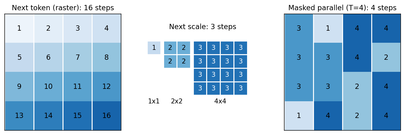
An order is a computational choice, not a claim about physics. Raster order (left to right, top to bottom) is convenient but arbitrary for a two-dimensional image: the pixel below you is just as related as the pixel to your right. Different orders lead to different conditionals, and a finite model may find some orders easier to learn than others. Figure 1 shows three prediction units used in this chapter.
Measuring an AR model: bits per dimension
Because the chain rule gives an exact , AR models are usually compared by negative log-likelihood in bits per dimension (bpd):
where is the number of discrete values in the image (for example for a RGB image) and converts nats to bits. A model that assigned every 8-bit value a uniform probability would score exactly 8 bpd; anything lower means the model has learned structure. Bpd is measured on held-out images, so it detects overfitting as well as underfitting.
Two cautions. First, bpd and visual quality can disagree: a model can spend most of its likelihood on imperceptible noise while still making odd global mistakes. Second, for a token model the likelihood is over codebook indices, not pixels. A lossy tokenizer throws information away, so a token-level likelihood is not an exact pixel-space likelihood and cannot be compared directly with pixel-model bpd.
Teacher forcing, causal masks and exposure bias
Plain version. Teacher forcing supplies the true prefix during training; sampling uses generated prefixes. Input shifts and masks must hide each prediction’s target.
With teacher forcing, every conditional in the training loss is computed using the ground-truth previous elements. Since the whole training image is available, all conditionals can be evaluated in a single forward pass, as long as position is prevented from reading positions . A causal transformer enforces this with an attention mask; a PixelCNN enforces it with masked convolution kernels.
Two input conventions are common, and the mask must match the convention:
- In a shifted-input decoder, feed
[BOS, x1, x2, ...]and predict[x1, x2, x3, ...]. A lower-triangular mask that includes the diagonal is correct, because the input at position is the previous element. - In a model that receives unshifted values, the dependency must be strictly earlier. Including the diagonal would let the network copy the value it is supposed to predict.
At inference, earlier sampled mistakes enter the context of later steps. This training/inference mismatch is often called exposure bias. It does not make maximum likelihood wrong (the factorization is still exact), but it matters in practice for imperfect models and long sequences: a small early error in the layout of an image can push later steps into contexts that never occurred in training.
Pixel models: PixelRNN and PixelCNN
Plain version. Treat each pixel’s intensity as a 256-way classification problem whose input is all pixels above and to the left.
PixelRNN and PixelCNN were introduced together by van den Oord, Kalchbrenner and Kavukcuoglu [2]. Both model each 8-bit value with a 256-way softmax rather than a Gaussian, so the distribution can be multimodal (a pixel can be “either black or white, but not grey”). Colour is handled by a fixed order inside each pixel, red then green then blue, so that green may depend on red and blue on both. PixelRNN uses two-dimensional LSTM layers (Row LSTM and Diagonal BiLSTM) whose dependency range is potentially unbounded; PixelCNN replaces them with stacked masked convolutions, which have a bounded receptive field but train much faster because all positions are computed in parallel.
Masked convolutions
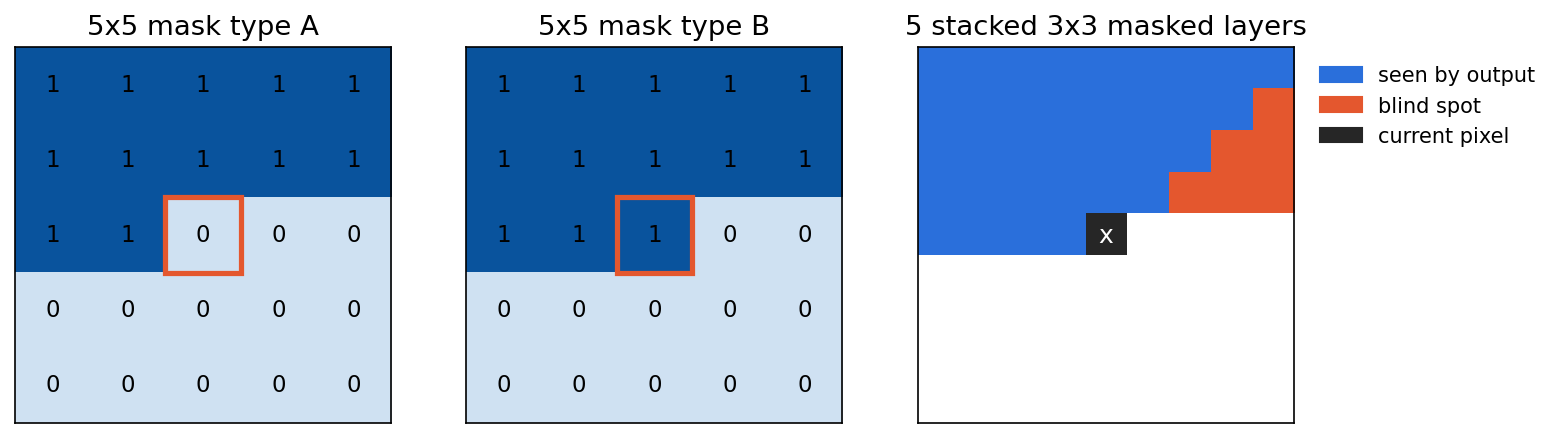
A masked convolution multiplies its kernel by a binary mask that zeros the weights at “future” positions. In [2], mask A is used only in the first layer: it excludes the centre pixel, so the first layer never sees the value it predicts (and, for colour, only sees channels already predicted). Mask B is used in all later layers: it allows the centre position, because after the first layer the centre feature already summarizes only earlier pixels. Formally, for a kernel with centre , ,
where indexes kernel rows and kernel columns. The code below builds both masks, stacks five layers, and uses a gradient to find exactly which input pixels can influence the output at the centre of a image.
Code · Python · 30 lines
import torch
from torch import nn
from torch.nn import functional as F

class MaskedConv2d(nn.Conv2d):
    """PixelCNN-style masked convolution for one channel (raster order)."""
    def __init__(self, cin, cout, k, mask_type):
        super().__init__(cin, cout, k, padding=k//2, bias=False)
        mask = torch.ones(k, k)
        c = k//2
        mask[c, c + (mask_type == "B"):] = 0   # centre (type A) and pixels to its right
        mask[c+1:] = 0                         # all rows below
        self.register_buffer("mask", mask)
    def forward(self, x):
        return F.conv2d(x, self.weight*self.mask, padding=self.padding)

torch.manual_seed(0)
layers = [MaskedConv2d(1, 8, 3, "A"), nn.Tanh()]
for _ in range(4):                            # 5 layers: reach of 5 pixels
    layers += [MaskedConv2d(8, 8, 3, "B"), nn.Tanh()]
net = nn.Sequential(*layers, MaskedConv2d(8, 1, 1, "B"))
print(net[0].mask.int())
x = torch.rand(1, 1, 9, 9, requires_grad=True)
net(x)[0, 0, 4, 4].backward()                 # logit for pixel (row 4, col 4)
dep = (x.grad[0, 0].abs() > 0).int()
print(dep)
later = torch.zeros(9, 9, dtype=torch.bool)
later[4, 4:] = True; later[5:] = True
assert dep[later].sum() == 0                  # never reads itself or later pixels
print("earlier pixels never seen (blind spot):", int(((dep == 0) & ~later).sum()))
The assertion passes: no pixel at or after the target influences its logit, so the model is a valid autoregressive factorization. But the printout reveals something else. Six pixels that come earlier in raster order, in a staircase above and to the right of the target, have zero gradient. This is the blind spot of stacked masked convolutions (Figure 2): each layer’s receptive field grows up and to the left, but the region up and to the right is never reached. The model is still correct, just less informed than it could be.
The Gated PixelCNN of van den Oord et al. [3] removed the blind spot by splitting the network into two stacks: a vertical stack that sees all rows above the current one without restriction and a horizontal stack that sees the current row up to the current pixel, combined after each layer. It also replaced ReLU with a gated unit , where is convolution, the logistic sigmoid and elementwise multiplication, and showed how to condition the model on class labels or embeddings. With these changes PixelCNN matched PixelRNN’s likelihood on ImageNet [23] at much lower cost [3].
Code: a minimal autoregressive model
Masked convolutions are one way to enforce causality; a transformer is not required either. The following complete CPU experiment generates binary images whose rows all repeat the same four random bits. A single masked linear layer, whose strictly lower-triangular mask excludes the current pixel and all later ones, learns the conditionals directly.
Code · Python · 34 lines
import torch
from torch import nn
from torch.nn import functional as F

torch.manual_seed(0)
torch.set_num_threads(1)
class BinaryAR(nn.Module):
    def __init__(self, n=16):
        super().__init__()
        self.weight = nn.Parameter(torch.zeros(n, n))
        self.bias = nn.Parameter(torch.zeros(n))
        self.register_buffer("mask", torch.tril(torch.ones(n, n), diagonal=-1))
    def forward(self, x):
        return F.linear(x, self.weight*self.mask, self.bias)

model = BinaryAR()
opt = torch.optim.Adam(model.parameters(), lr=.04)
for step in range(600):
    first_row = torch.randint(2, (128, 4)).float()
    x = first_row.repeat(1, 4)
    loss = F.binary_cross_entropy_with_logits(model(x), x)
    opt.zero_grad(); loss.backward(); opt.step()

with torch.no_grad():
    a = torch.rand(2, 16)
    b = a.clone(); b[:, 8:] = torch.rand(2, 8)
    assert torch.allclose(model(a)[:, :9], model(b)[:, :9])
    samples = torch.zeros(8, 16)
    for i in range(16):
        p = model(samples)[:, i].sigmoid()
        samples[:, i] = torch.bernoulli(p)
    rows = samples.reshape(-1, 4, 4)
    print("one generated image:\n", rows[0].int())
    print("repeat agreement:", (rows[:, 1:] == rows[:, :1]).float().mean().item())
The assertion checks causality: changing positions 8 onward cannot alter the logits for positions 0 through 8, because each of those outputs reads only earlier inputs. Training then drives the agreement between later rows and the first row to 1.0, while the first row stays random (the model must not memorize one particular row).
The true distribution has 16 equally likely images, so its entropy is bits per image, or 0.25 bits per pixel. Later rows contain no new uncertainty. A model that treated all 16 pixels as independent fair coins would need 16 bits per image. The gap between 16 and 4 bits is exactly the structure an autoregressive model captures and an independent-pixel model cannot.
Why pixel models stopped scaling
A RGB image has values, so pixel-level sampling needs about two hundred thousand sequential network evaluations. Most of the likelihood is also spent on fine, locally predictable detail, while the global layout that people notice is a small fraction of the bits. Image GPT [11] showed that a plain sequence transformer trained to predict pixels autoregressively on low-resolution images learns features that transfer well under linear probing, but the pixel route stays expensive at higher resolutions. The next step was to learn a shorter, more meaningful sequence.
Discrete visual tokens: VQ-VAE and VQGAN
Plain version. Train a separate network that compresses an image into a small grid of “words” from a learned dictionary, then do autoregression over the words instead of the pixels.
VQ-VAE
VQ-VAE [4] has an encoder that produces a feature vector at each position of a downsampled grid, a codebook of learned vectors, and a decoder. Each feature is replaced by its nearest code:
The image is now represented by the integer grid of values. Training minimizes
where is the decoder, is the stop-gradient operator (identity in the forward pass, zero gradient in the backward pass), and is a small weight on the commitment term (the snippet below uses 0.25). The reconstruction term is written as squared error here; any reconstruction likelihood can take its place.
The three terms do three jobs. The codebook term moves the chosen code toward the encoder output, like a k-means update. The commitment term pulls the encoder toward its code so that encoder outputs do not drift far from the codebook. The argmin has no useful gradient, so the reconstruction gradient reaches the encoder through the straight-through estimator: in the forward pass use , in the backward pass copy the gradient from to as if quantization were the identity. In code this is the one-liner z_q = z_e + (e - z_e).detach().
The toy below trains a 2-D “encoder”, codebook and decoder on four clusters, with eight codes available:
Code · Python · 37 lines
import torch
from torch import nn
from torch.nn import functional as F

def quantize(z_e, codebook, beta=0.25):
    """z_e: (n, d) encoder outputs; codebook: (K, d). Returns z_q with straight-through gradient."""
    dist = torch.cdist(z_e, codebook)            # (n, K) Euclidean distances
    idx = dist.argmin(1)                         # nearest code index per vector
    e = codebook[idx]
    codebook_loss = F.mse_loss(e, z_e.detach())  # moves codes toward encoder outputs
    commit_loss = F.mse_loss(z_e, e.detach())    # keeps the encoder near its code
    z_q = z_e + (e - z_e).detach()               # forward: e; backward: identity
    return z_q, idx, codebook_loss + beta*commit_loss

torch.manual_seed(0)
torch.set_num_threads(1)
centres = torch.tensor([[2., 0.], [-2., 0.], [0., 2.], [0., -2.]])
encoder = nn.Linear(2, 2)                        # toy "encoder" and "decoder"
decoder = nn.Linear(2, 2)
codebook = nn.Parameter(torch.randn(8, 2)*.1)    # K = 8 codes, 4 are enough
opt = torch.optim.Adam([*encoder.parameters(), *decoder.parameters(), codebook], lr=.03)
for step in range(800):
    x = centres[torch.randint(4, (256,))] + .1*torch.randn(256, 2)
    z_q, idx, vq_loss = quantize(encoder(x), codebook)
    loss = F.mse_loss(decoder(z_q), x) + vq_loss
    opt.zero_grad(); loss.backward(); opt.step()

with torch.no_grad():
    x = centres.repeat_interleave(100, 0) + .1*torch.randn(400, 2)
    z_q, idx, _ = quantize(encoder(x), codebook)
    print("reconstruction MSE:", round(F.mse_loss(decoder(z_q), x).item(), 4))
    print("codes used:", idx.unique().numel(), "of", len(codebook))
    print("codes per cluster:", [idx[i*100:(i+1)*100].unique().tolist() for i in range(4)])
z = torch.randn(3, 2, requires_grad=True)
z_q, _, _ = quantize(z, codebook.detach())
z_q.sum().backward()
print("straight-through gradient:", z.grad[0].tolist())
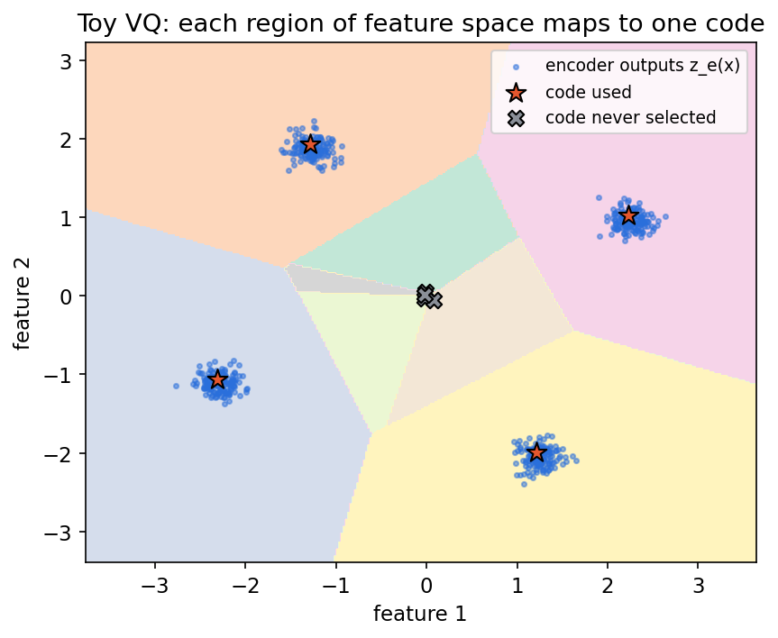
It prints a reconstruction MSE of about 0.0096, uses 4 of the 8 codes (one per cluster), and shows a straight-through gradient of [1.0, 1.0]. Two lessons hide in those numbers. The reconstruction error is almost exactly the within-cluster noise variance : quantization has kept which cluster and discarded where inside the cluster. And half the codebook is dead: codes that are never selected receive no codebook gradient and never move (Figure 3). In real tokenizers, low codebook usage wastes capacity and is a standard failure to monitor.
Two stages: a tokenizer, then a prior
A VQ-VAE alone is an autoencoder; it does not by itself say which token grids are likely. Generation therefore has two stages (Figure 4). Stage 1 trains the tokenizer. Stage 2 freezes it, converts every training image into its index grid, and trains an autoregressive model over the indices. To sample, draw an index grid from the prior and decode it. In [4] the prior was a PixelCNN over codes; VQ-VAE-2 [10] used a hierarchy of two code maps (a coarse top level and a finer bottom level) with PixelCNN-style priors and produced diverse, high-fidelity ImageNet samples.
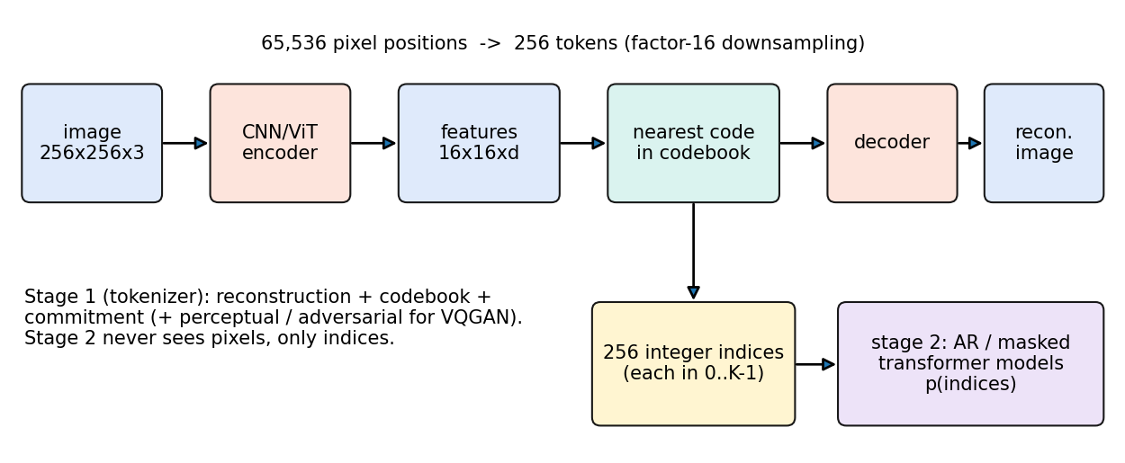
The arithmetic explains the appeal. If a tokenizer downsamples a image by 16 in each direction, the prior sees tokens rather than 65,536 pixel positions (or 196,608 colour values). Self-attention cost grows with the square of sequence length, so this is the difference between feasible and infeasible.
VQGAN: perceptual tokens
Esser, Rombach and Ommer’s VQGAN [5] kept the two-stage design but trained the tokenizer with a perceptual loss and a patch-based adversarial loss in addition to reconstruction, and modelled the token grid with a transformer. The adversarial and perceptual terms let the decoder produce sharp, realistic texture from very few tokens, because the tokens no longer need to encode every pixel exactly; they need to encode enough for the decoder to produce a plausible version. This is why VQGAN-style tokenizers became the default front end for token-based generation. Note the division of labour: the tokenizer uses adversarial training, but the prior is an ordinary autoregressive model trained by maximum likelihood.
Codebook problems and alternatives
Real tokenizers face three recurring problems: dead codes (as in the toy), a gap between what the tokenizer reconstructs and what the prior can model, and loss of small details such as text and thin lines. Several designs respond to them:
- ViT-VQGAN [12] uses a Vision Transformer encoder/decoder, looks codes up in a low-dimensional factorized space and -normalizes codes and features, which improved codebook usage and reconstruction.
- RQ-VAE [15] uses residual quantization: each position is represented by a short stack of codes, each one quantizing what the previous ones missed. This allows a coarser spatial grid (shorter sequence) at similar fidelity.
- FSQ [16] (finite scalar quantization) projects to a handful of dimensions and rounds each to a few fixed levels. The implicit codebook is the product of the levels; there is no learned codebook to collapse and no commitment loss.
Compression always creates a bottleneck. Measure codebook usage, reconstruction quality and the generator’s quality separately: a generator cannot produce detail its tokenizer cannot represent.
Optional: VQ-VAE (in the Paper guides). Read the original figure, evidence, design choices and limitations.
Autoregressive transformers over tokens
Plain version. A decoder-only Transformer can predict the next visual token as it predicts a text token. The visual tokenizer and decoder determine what those tokens represent.
From pixels to tokens
Image GPT [11] applied a GPT-style transformer directly to sequences of low-resolution pixels. Its main finding was about representation learning: features from a model trained only to predict the next pixel transfer well when a linear classifier is trained on top. Working on tokens instead of pixels shortens sequences enough to generate at higher resolution. The VQGAN transformer [5] is the classic example: a GPT-like model over VQGAN indices in raster order, which let a transformer synthesize high-resolution images that would be far too long as pixel sequences.
Text-to-image as translation: Parti
Parti [13] treats text-to-image generation like machine translation. A transformer encoder reads the text prompt; a transformer decoder autoregressively generates ViT-VQGAN image tokens [12] conditioned on it. The report scales this sequence-to-sequence model up to 20 billion parameters and introduces PartiPrompts, a benchmark of more than 1,600 English prompts spanning many categories of content.
Language-model architecture, unchanged: LlamaGen
LlamaGen [14] asks whether a vanilla language-model architecture, with no image-specific inductive biases, can generate images well when scaled. It uses a Llama-style [24] decoder (RMSNorm pre-normalization, SwiGLU feed-forward layers, 2-D rotary position embeddings) over the tokens of a factor-16 VQ tokenizer with codes of dimension 8. The class label or projected text embedding is supplied as a prefix token, and generation proceeds in raster order. The paper releases class-conditional models from 111M to 3.1B parameters and reports that standard LLM serving software (vLLM) speeds up inference. Its broader message is architectural reuse: an image generator can share almost everything with a text model except the tokenizer.
Classifier-free guidance for autoregressive models
Classifier-free guidance (CFG) [18] was introduced for diffusion models, but it transfers directly to AR logits. During training, the condition is randomly replaced by a learned null embedding so that one network learns both conditional and unconditional predictions. At each sampling step, compute both sets of logits and combine them:
where are the next-token logits with the condition, the logits with the null condition, and the guidance scale; recovers the ordinary conditional model. This is the form LlamaGen uses [14]. Larger usually improves prompt or class adherence and sample sharpness at the cost of diversity. It also doubles the per-step compute unless the two passes are batched, so step counts alone understate cost.
Next-scale prediction (VAR)
Plain version. Instead of predicting the next token in a fixed reading order, predict the next, sharper version of the whole image, conditioned on all coarser versions.
Raster order forces a strange dependency: the top-left of an image is generated without any knowledge of the bottom-right. VAR (Visual AutoRegressive modeling) [6] argues that this one-directional order conflicts with the two-directional correlations of image tokens and with spatial locality, and replaces it with a coarse-to-fine order over token maps of increasing resolution:
where is an grid of token indices, is and has the full latent resolution. All tokens of are predicted in parallel given the coarser maps, so the number of sequential steps equals the number of scales, not the number of tokens.
The tokenizer is part of the method. VAR’s multi-scale VQ encoder works residually: starting from the encoder feature map , for it downsamples to , quantizes it to get (with one codebook shared across scales), upsamples the looked-up codes back to full resolution, passes them through a small convolution , and subtracts the result from before moving to the next scale [6]. Each scale therefore encodes what the coarser scales have not explained. Simply resizing ordinary token maps would not reproduce this.
During training, a block-wise causal attention mask lets every token of attend to all tokens of but none of the finer scales; at inference a KV cache stores the coarser scales. VAR uses CFG as well. On class-conditional ImageNet the paper reports that VAR improves its AR baseline’s FID from 18.65 to 1.73, with faster inference, and that its models follow power-law scaling trends similar to those of language models [6]. VAR received a NeurIPS 2024 Best Paper award. As always, those numbers apply to the paper’s data, resolution and training protocol.
Parallel prediction within a scale is itself an assumption: tokens in are sampled independently given . The masked-model section shows what that assumption can cost on a toy problem.
Masked generative models (MaskGIT and Muse)
Plain version. Start with a grid of blanks. At each round, guess every blank at once, keep only the guesses you are most confident about, and blank out the rest again.
MaskGIT [8] uses the same VQ tokens as an AR model, but a bidirectional transformer that sees every position. Training is a masked-token objective: choose a mask ratio, replace that fraction of tokens with a special [MASK] token, and minimize cross-entropy on the masked positions,
where is the token grid, is the set of masked positions and the unmasked tokens. The mask ratio is drawn as with and a mask schedule that decreases from 1 to 0.
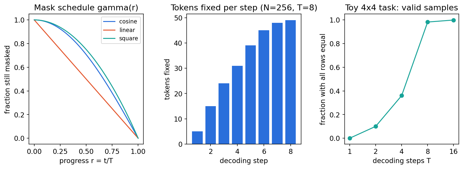
Generation runs for iterations. At iteration the model predicts all masked tokens in parallel and samples them; each sample’s probability serves as its confidence. The number of tokens that remain masked after the iteration is
with the total number of tokens, so the least confident new tokens are re-masked and everything else is fixed. MaskGIT compares several schedules and selects the cosine schedule , which fixes few tokens early (when the model knows little) and many late; it generates images in 8 iterations with a 16×16 token grid and a 1,024-entry codebook [8]. Muse [17] scales the same idea to text-to-image generation, conditioning the masked-token transformer on text embeddings from a pre-trained large language model.
MaskGIT is not ordinary left-to-right chain-rule autoregression: the order is chosen on the fly by confidence, and several tokens are sampled in the same step. Those simultaneous tokens are drawn independently given the current context. The toy below shows when that matters. It trains a small bidirectional network on the repeated-row images from earlier and decodes with the cosine schedule.
Code · Python · 49 lines
import math
import torch
from torch import nn
from torch.nn import functional as F

torch.manual_seed(0)
torch.set_num_threads(1)
N, MASK = 16, 2                                   # 16 binary tokens; state 2 = [MASK]
gamma = lambda r: math.cos(math.pi*r/2)          # cosine schedule: fraction still masked
net = nn.Sequential(nn.Flatten(), nn.Linear(3*N, 128), nn.ReLU(), nn.Linear(128, N))

def data(n):                                      # 4x4 images whose rows repeat
    return torch.randint(2, (n, 4)).repeat(1, 4)

def logits(tokens):                               # sees every position: bidirectional
    return net(F.one_hot(tokens, 3).float())

opt = torch.optim.Adam(net.parameters(), lr=3e-3)
for step in range(1500):
    x = data(256)
    ratio = torch.tensor([gamma(r) for r in torch.rand(256).tolist()])
    n_mask = (ratio*N).ceil().clamp(min=1)
    masked = torch.rand(256, N).argsort(1) < n_mask[:, None]   # random positions
    inp = torch.where(masked, MASK, x)
    loss = F.binary_cross_entropy_with_logits(logits(inp)[masked], x[masked].float())
    opt.zero_grad(); loss.backward(); opt.step()

@torch.no_grad()
def generate(n, T=4):
    tokens = torch.full((n, N), MASK)
    for t in range(1, T+1):
        p = logits(tokens).sigmoid()
        sample = torch.bernoulli(p).long()
        conf = torch.where(sample == 1, p, 1-p)               # prob. of the drawn value
        still = tokens == MASK
        conf = torch.where(still, conf, torch.inf)            # never re-mask fixed tokens
        proposal = torch.where(still, sample, tokens)
        n_keep_masked = math.floor(gamma(t/T)*N)              # 0 after the last step
        order = conf.argsort(1)                               # least confident first
        remask = torch.zeros_like(still)
        remask.scatter_(1, order[:, :n_keep_masked], True)
        tokens = torch.where(remask, MASK, proposal)
    return tokens

for T in (1, 2, 4, 8, 16):
    rows = generate(1000, T).reshape(-1, 4, 4)
    agree = (rows[:, 1:] == rows[:, :1]).float().mean().item()
    valid = (rows == rows[:, :1]).all(2).all(1).float().mean().item()
    print(f"T={T:2d}  repeat agreement={agree:.3f}  valid images={valid:.3f}")
(The code uses floor rather than the paper’s ceiling so that the count reaches exactly zero at in this tiny example.) The output is:
Code · 5 lines
T= 1  repeat agreement=0.511  valid images=0.000
T= 2  repeat agreement=0.812  valid images=0.100
T= 4  repeat agreement=0.908  valid images=0.360
T= 8  repeat agreement=0.998  valid images=0.982
T=16  repeat agreement=1.000  valid images=0.999
With every token is sampled independently from the all-mask context, so rows almost never agree. With more iterations, the first few tokens are fixed early and later ones can condition on them; by nearly every sample is valid. On natural images the dependence between tokens decoded in the same round is weaker, which is why a handful of iterations works, but the trade-off between fewer steps and more independence assumptions is real (Figure 5).
Continuous tokens and diffusion conditionals (MAR)
Plain version. Autoregression defines the conditioning order; a small diffusion model can represent each continuous-token conditional distribution.
Vector quantization is lossy and awkward to train. Li et al. [7] observe that autoregression needs a way to model , not necessarily a categorical distribution. They let the AR (or masked AR) transformer output a conditioning vector for each continuous-valued token , and train a small MLP denoiser with a diffusion loss:
where , is a diffusion time step and the noise schedule from ML 08. The gradient also flows into the transformer through . To sample a token, run the reverse diffusion process of the small denoiser conditioned on ; a temperature scales the injected noise. The paper’s main variant, MAR (masked autoregressive), uses a random order and predicts a set of tokens per step, combining the outer structure of MaskGIT with an inner continuous sampler [7].
Consequently, “AR versus diffusion” is not an either/or choice. A system can decide the order and grouping of tokens autoregressively and sample each group by diffusion. Likewise, a language decoder can autoregressively generate text about an image without generating any pixels; the unifying idea is factorization, not a particular output type.
Sampling, temperature and caching
Plain version. The trained model gives a distribution at every step; the sampler decides how adventurous to be when drawing from it, and the cache avoids recomputing the past.
For logits over possible values, temperature rescales the distribution:
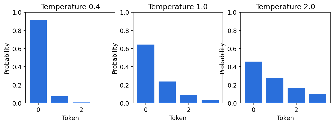
Lower concentrates probability on the top values; larger spreads it (Figure 6). Top- sampling keeps only the highest logits; top- (nucleus) sampling keeps the smallest set of values whose probability mass reaches . Both renormalize what remains.
Code · Python · 22 lines
import torch

def filtered_probs(logits, temperature=1.0, top_k=None, top_p=None):
    """Return the (renormalized) distribution actually sampled from."""
    logits = logits / temperature
    if top_k is not None:                               # keep the k largest logits
        kth = logits.topk(top_k).values[..., -1, None]
        logits = logits.masked_fill(logits < kth, -torch.inf)
    if top_p is not None:                               # smallest set with mass >= p
        sorted_logits, order = logits.sort(descending=True)
        cum = sorted_logits.softmax(-1).cumsum(-1)
        drop = cum - sorted_logits.softmax(-1) >= top_p  # mass before this token already >= p
        sorted_logits = sorted_logits.masked_fill(drop, -torch.inf)
        logits = torch.empty_like(logits).scatter(-1, order, sorted_logits)
    return logits.softmax(-1)

logits = torch.tensor([2.0, 1.0, 0.0, -1.0])
for name, kw in [("T=1", {}), ("T=0.5", {"temperature": .5}), ("T=2", {"temperature": 2.}),
                 ("top-k=2", {"top_k": 2}), ("top-p=0.8", {"top_p": .8})]:
    p = filtered_probs(logits, **kw)
    entropy = -(p[p > 0]*p[p > 0].log2()).sum().item()
    print(f"{name:10s}", [round(v, 3) for v in p.tolist()], f"entropy={entropy:.2f} bits")
The model’s own distribution () has 1.37 bits of entropy; lowers it to 0.66 bits and raises it to 1.80 bits. Top- and top- both keep the two most likely values here (the first value has mass 0.644, which is below 0.8, so the second is needed). Every one of these changes the distribution you sample from, so a sampler’s visual quality should not be confused with the model’s likelihood.
The KV cache
In a causal transformer, the keys and values of earlier tokens do not change when a new token is appended. A KV cache stores them, so each new step computes the query, key and value of the newest token only and attends to the cache:
Code · Python · 24 lines
import torch
from torch.nn import functional as F

torch.manual_seed(0)
d, n = 8, 6
Wq, Wk, Wv = (torch.randn(d, d) for _ in range(3))
x = torch.randn(n, d)                                 # embeddings of n tokens

# Full causal attention over the whole sequence (what training computes).
q, k, v = x@Wq, x@Wk, x@Wv
mask = torch.ones(n, n).tril().bool()
scores = (q@k.T/d**.5).masked_fill(~mask, -torch.inf)
full = scores.softmax(-1)@v

# Incremental decoding: each step computes q, k, v for the newest token only.
K_cache, V_cache, outputs = [], [], []
for i in range(n):
    K_cache.append(x[i]@Wk); V_cache.append(x[i]@Wv)
    K, V = torch.stack(K_cache), torch.stack(V_cache)
    att = F.softmax((x[i]@Wq)@K.T/d**.5, -1)        # attends to tokens 0..i
    outputs.append(att@V)
assert torch.allclose(full, torch.stack(outputs), atol=1e-5)
print("cached decoding matches full causal attention")
print("dot products per step:", [i+1 for i in range(n)], "total:", n*(n+1)//2)
The assertion confirms that cached decoding gives exactly the training-time causal outputs (for a single layer here; real models cache every layer and head). The cache removes recomputation but not the sequential dependency, and it grows linearly with sequence length. Step still attends to cached keys, so total attention work over a sequence of length is , quadratic in . This is why shorter sequences (better tokenizers) and fewer sequential steps (next-scale or masked decoding) matter so much.
For video, tokens can be ordered over space and time or grouped into chunks. Caching, compression and temporal ordering then dominate cost, and object consistency and long-duration drift need their own evaluation.
Autoregressive versus diffusion
Plain version. Both families turn one hard generation problem into many easier ones. AR splits the image into pieces; diffusion splits the noise level into steps.
| Aspect | Autoregressive (token / scale) | Masked generative | Diffusion / flow (ML 08) |
|---|---|---|---|
| What is generated per step | One token (or one scale) | A confidence-chosen set of tokens | A refinement of the whole sample |
| Sequential steps | Tokens or scales | Fixed, typically few () | Solver steps (NFE) |
| Typical representation | Discrete codes (or continuous with a diffusion head [7]) | Discrete codes | Continuous pixels or latents |
| Training objective | Exact NLL (cross-entropy) | Masked cross-entropy | Denoising / velocity regression (ELBO-related) |
| Likelihood | Exact over tokens | Not a single exact chain-rule likelihood | Bound or ODE-based estimate |
| Natural strengths | Shares architecture and serving with LLMs; mixes with text | Few steps; easy inpainting and editing | Strong image quality; flexible guidance |
| Typical weaknesses | Long sequential decoding; tokenizer bottleneck; error accumulation | Independence within a step | Many network evaluations unless distilled |
Three points keep this table honest. First, the families mix: MAR [7] puts a diffusion model inside an AR loop, and latent diffusion also depends on a learned tokenizer-like autoencoder. Second, claims that one family “beats” the other (as in LlamaGen’s title [14] or VAR’s comparison with DiT [6]) hold for a stated benchmark, tokenizer, model size and guidance setting, not universally. Third, cost should be compared in network evaluations, guidance passes, sequence length and actual latency, not in “steps” alone.
Modern view
The field has moved from raw pixels to learned representations, from fixed raster order to flexible prediction units, and from separate image generators to models that read and write both text and images. Several surveys map this territory:
- Xiong et al. [1] (TMLR) is the most direct survey of visual autoregression. Its taxonomy by representation (pixel-, token- and scale-based models) is the one used in this chapter, and it covers applications in image, video, 3D and multimodal generation as well as embodied and medical settings.
- Bond-Taylor et al. [19] (TPAMI 2022) compare VAEs, GANs, normalizing flows, energy-based and autoregressive models side by side, including the trade-offs in run time, sample diversity and architectural constraints. It places AR models in the wider generative-model landscape: exact likelihood and stable training, paid for with slow sequential sampling.
- Li et al. [20] (TPAMI 2026) survey discrete tokenization for multimodal LLMs, organizing vector-quantization variants and their use in classical, single-modality LLM and multimodal LLM systems, and discussing codebook collapse and unstable gradient estimation.
- Jia et al. [22] survey discrete tokenizers across generation, comprehension, recommendation and retrieval, dissecting tokenizers into their sub-modules and mechanisms before organizing methods by application, and listing limitations and future directions.
- Zhao et al. [21] survey unified multimodal understanding-and-generation models, grouping them into diffusion-based, autoregressive-based and hybrid AR–diffusion designs, which is where most 2025–2026 activity sits.
State of the art (2023–2026). Three lines stand out in the verified literature. (i) Scaling plain AR transformers over better tokenizers: LlamaGen [14] shows that a language-model architecture with almost no image-specific design is competitive on class-conditional ImageNet when the tokenizer and training are good. (ii) Changing the prediction unit: VAR’s next-scale prediction [6] and masked decoding in MaskGIT and Muse [8], [17] reduce the number of sequential steps; MAR [7] removes vector quantization by using a diffusion head per token. (iii) Unified multimodal models: the same next-token machinery is used to generate text and image tokens in one model, with tokenizers designed to serve both understanding and generation [20], [21]. Our interpretation is that choosing the representation and prediction unit now matters at least as much as choosing the backbone.
Open problems. The surveys repeatedly point to the following:
- Tokenizer quality. Reconstruction caps generation quality; small text, faces and fine geometry are the usual casualties. Better codebook usage and semantic structure without losing detail remain active topics [20], [22].
- Discrete versus continuous tokens. Discrete tokens fit LLM machinery; continuous tokens reconstruct better but need a continuous conditional model such as a diffusion head [7].
- Speed. Sequential decoding is latency-bound. Next-scale, masked and parallel decoding trade steps for independence assumptions.
- Evaluation. Token likelihood, FID-type metrics, prompt adherence and human preference measure different things; a lossy tokenizer’s token likelihood is not a pixel likelihood.
- Video and long contexts. Token counts explode over time, and temporal consistency, object permanence and drift need dedicated evaluation [1].
Key takeaways
- Autoregression is a distribution factorization; it does not prescribe a Transformer architecture.
- Teacher forcing supplies true prefixes; causal masks and shifted inputs must prevent target leakage.
- Tokenization shortens sequences while constraining the decoder’s representational capacity.
- Token, scale and masked prediction use different factorizations or update rules; compare their dependency assumptions.
- Temperature and truncation change sampling probabilities; caching reuses computation without changing the intended conditional distribution.
- Compare autoregressive and diffusion pipelines using matched data, representations, guidance and cost.
Exercises
- Leak the answer. Change the
BinaryARmask to include the diagonal (diagonal=0). Explain why the training loss can fall almost to zero while sampling breaks.
Hint
Each output can now read its own target and simply copy it, so the training loss collapses. At sampling time the current position is still 0 (not yet drawn) when its logit is computed, so the learned “copy” rule produces nonsense. The causality assertion in the snippet would also fail.
- Bits per dimension. For the repeated-row binary data, compute the bits per pixel of (a) the true distribution, (b) a model that treats every pixel as an independent fair coin, and (c) a model that learns the first row perfectly but treats later rows as independent fair coins.
Hint
(a) 4 bits / 16 pixels = 0.25. (b) 16 / 16 = 1.0. (c) 4 + 12 = 16 bits per image, also 1.0 bits per pixel: learning the first row’s marginal does not help, because its bits are already uniform. All gains come from modelling the dependence of later rows on the first.
- Tokenizer budget. A image is tokenized with factor-8 or factor-16 downsampling. Compute the sequence length in each case and the ratio of full self-attention costs. What might you lose with factor 16?
Hint
versus tokens. Attention cost scales with length squared, so the ratio is 16. With factor 16 each token must describe a patch, so small text and thin structures are more likely to be lost unless the codebook or decoder compensates.
- Blind spot. Modify the masked-convolution snippet to use 7 layers and an input with the target at the centre. How many earlier pixels are never seen? Then sketch how a vertical stack plus a horizontal stack removes them.
Hint
The blind spot is the staircase above and to the right of the target that the up-left-growing receptive field never reaches; counting zero-gradient cells that are earlier in raster order gives 10. A vertical stack sees full rows above (no left/right restriction) and is fed into the horizontal stack, which handles the current row only, so every earlier pixel becomes reachable.
- Masked decoding steps. Using with the cosine schedule, and , compute how many tokens are fixed at each step. Why does the schedule fix few tokens first?
Hint
Remaining masked counts are 252, 237, 213, 182, 143, 98, 50 and 0, so 4, 15, 24, 31, 39, 45, 48 and 50 tokens are fixed per step (the figure uses floor, which shifts counts by at most one). In exact arithmetic ; in floating point is a tiny positive number, so a literal ceiling leaves one token masked, another reason the snippet uses floor. Early on the model has little context, so its parallel guesses are the least reliable and the most likely to conflict; fixing only a few lets later steps condition on them.
- Classify the methods. For PixelCNN, VQGAN transformer, Parti, LlamaGen, VAR, MaskGIT and MAR, give the prediction unit, the representation (pixels, discrete tokens, continuous tokens, multiscale maps), the conditional distribution type, and the number of sequential steps for a token grid.
Hint
PixelCNN: pixels in raster order, 256-way softmax, one step per value. VQGAN transformer, Parti, LlamaGen: discrete tokens in raster order, softmax over the codebook, 256 steps. VAR: multiscale discrete maps, softmax per token with parallel tokens inside a scale, one step per scale. MaskGIT: discrete tokens, bidirectional masked prediction, steps (8 in the paper). MAR: continuous tokens in random-order groups, a per-token diffusion head, as many steps as groups (each with its own inner diffusion steps).
References
- J. Xiong, G. Liu, L. Huang et al., “Autoregressive Models in Vision: A Survey,” Transactions on Machine Learning Research (TMLR), 2025 (arXiv:2411.05902, 2024). arXiv
- A. van den Oord, N. Kalchbrenner and K. Kavukcuoglu, “Pixel Recurrent Neural Networks,” in Proc. ICML, PMLR 48, 2016. PMLR
- A. van den Oord, N. Kalchbrenner, O. Vinyals, L. Espeholt, A. Graves and K. Kavukcuoglu, “Conditional Image Generation with PixelCNN Decoders,” in NeurIPS, 2016. NeurIPS
- A. van den Oord, O. Vinyals and K. Kavukcuoglu, “Neural Discrete Representation Learning,” in NeurIPS, 2017. NeurIPS
- P. Esser, R. Rombach and B. Ommer, “Taming Transformers for High-Resolution Image Synthesis,” in Proc. IEEE/CVF CVPR, 2021. CVF
- K. Tian, Y. Jiang, Z. Yuan, B. Peng and L. Wang, “Visual Autoregressive Modeling: Scalable Image Generation via Next-Scale Prediction,” in NeurIPS, 2024 (Best Paper Award). arXiv
- T. Li, Y. Tian, H. Li, M. Deng and K. He, “Autoregressive Image Generation without Vector Quantization,” in NeurIPS, 2024. arXiv
- H. Chang, H. Zhang, L. Jiang, C. Liu and W. T. Freeman, “MaskGIT: Masked Generative Image Transformer,” in Proc. IEEE/CVF CVPR, 2022. CVF
- S. J. D. Prince, Understanding Deep Learning, MIT Press, 2023. Book
- A. Razavi, A. van den Oord and O. Vinyals, “Generating Diverse High-Fidelity Images with VQ-VAE-2,” in NeurIPS, 2019. NeurIPS
- M. Chen, A. Radford, R. Child, J. Wu, H. Jun, D. Luan and I. Sutskever, “Generative Pretraining From Pixels,” in Proc. ICML, PMLR 119, 2020. PMLR
- J. Yu, X. Li, J. Y. Koh et al., “Vector-quantized Image Modeling with Improved VQGAN,” in ICLR, 2022. arXiv
- J. Yu, Y. Xu, J. Y. Koh et al., “Scaling Autoregressive Models for Content-Rich Text-to-Image Generation,” Transactions on Machine Learning Research, 2022. arXiv
- P. Sun, Y. Jiang, S. Chen, S. Zhang, B. Peng, P. Luo and Z. Yuan, “Autoregressive Model Beats Diffusion: Llama for Scalable Image Generation,” arXiv:2406.06525, 2024. arXiv
- D. Lee, C. Kim, S. Kim, M. Cho and W.-S. Han, “Autoregressive Image Generation using Residual Quantization,” in Proc. IEEE/CVF CVPR, 2022. CVF
- F. Mentzer, D. Minnen, E. Agustsson and M. Tschannen, “Finite Scalar Quantization: VQ-VAE Made Simple,” in Proc. International Conference on Learning Representations (ICLR), 2024. arXiv
- H. Chang, H. Zhang, J. Barber et al., “Muse: Text-To-Image Generation via Masked Generative Transformers,” in Proc. ICML, PMLR 202, 2023. PMLR
- J. Ho and T. Salimans, “Classifier-Free Diffusion Guidance,” arXiv:2207.12598, 2022 (short version at the NeurIPS 2021 Workshop on Deep Generative Models and Downstream Applications). arXiv
- S. Bond-Taylor, A. Leach, Y. Long and C. G. Willcocks, “Deep Generative Modelling: A Comparative Review of VAEs, GANs, Normalizing Flows, Energy-Based and Autoregressive Models,” IEEE TPAMI, vol. 44, no. 11, 2022. doi
- J. Li, Y. Fu, J. Liu, L. Cao, W. Ji, M. Yang, I. King and M.-H. Yang, “Discrete Tokenization for Multimodal LLMs: A Comprehensive Survey,” IEEE TPAMI, 2026 (arXiv:2507.22920). doi
- S. Zhao, X. Zhang, J. Guo et al., “Unified Multimodal Understanding and Generation Models: Advances, Challenges, and Opportunities,” arXiv:2505.02567, 2025; revised 2026. arXiv
- J. Jia, J. Gao, B. Xue et al., “From Principles to Applications: A Comprehensive Survey of Discrete Tokenizers in Generation, Comprehension, Recommendation, and Information Retrieval,” arXiv:2502.12448, 2025. arXiv
- J. Deng, W. Dong, R. Socher, L.-J. Li, K. Li and L. Fei-Fei, “ImageNet: A Large-Scale Hierarchical Image Database,” CVPR, 2009, pp. 248–255. doi
- H. Touvron, T. Lavril, G. Izacard et al., “LLaMA: Open and Efficient Foundation Language Models,” arXiv:2302.13971, 2023. arXiv
Check your understanding
This tutorial has 6 exercises. Can you solve them without opening the hints?
Go to the exercises ↑Next ML 10 · Foundation Models and Vision–Language Learning · 27 min