ML 03 · Convolution, Image Filtering and CNNs
Needs: ML 02 · Neural Networks from Perceptron to Deep Networks, Images as Arrays
Navigate: this page and this track: Navigate: this page and this track
Explore this chapter 2 interactive experiments
Predict the response of flat regions and edges as you change the kernel weights.
What you’ll learn
- Explain filtering kernels and distinguish correlation from convolution.
- Implement filtering with explicit data types and border rules.
- Track channels, padding, stride, dilation and output shapes.
- Relate receptive fields, translation behavior and backpropagation.
- Compare CNN designs through their structural and computational choices.
The big picture
An image is a grid of numbers (see Images as arrays). Many of the most useful things we can do to it are local: whether a pixel sits on an edge, inside a smooth region or in a noisy patch depends mostly on its neighbors. Convolution is the operation that formalizes “look at a small neighborhood, combine it with fixed weights, and repeat everywhere.” It is the workhorse of classical image processing, and it is also the building block of convolutional neural networks (CNNs), which learn their weights from data instead of having them designed by hand.
This tutorial has two halves. The first half (filtering) is the classical toolbox and needs only NumPy. The second half (CNNs) builds on ML 02, where you met layers, losses and backpropagation. If you want more depth on fixed filters afterward, IP 03 covers spatial filtering and IP 04 explains the frequency-domain view through the convolution theorem. For the deep-learning side, DLCV 02 studies modern classification backbones in detail, ML 04 turns to sequences, and ML 05 introduces attention, the main alternative to convolution. Standard textbook treatments are chapter 9 of Goodfellow et al. [1] and chapter 10 of Prince [10].
Part I · Filtering with a fixed kernel
The sliding weighted sum
Plain version. Every output pixel is a weighted sum of the input pixels around the same position. The small grid of weights is called a kernel (also filter or mask).
Precise version. Let be a grayscale image, with the intensity at column and row . Let be a kernel of size , indexed from to vertically and to horizontally, so that is its center. The filtered image is
Here indexes kernel rows and kernel columns, is the output at the same position, and the double sum visits every tap of the kernel once. For a kernel, and each output pixel costs nine multiplications and eight additions.
Figure 1 works through one output value by hand. The orange window covers the top-left neighborhood of the padded input. Multiply element-wise by the kernel and add: . That number becomes at the window’s center. Sliding the window one step to the right and repeating fills in the next output.
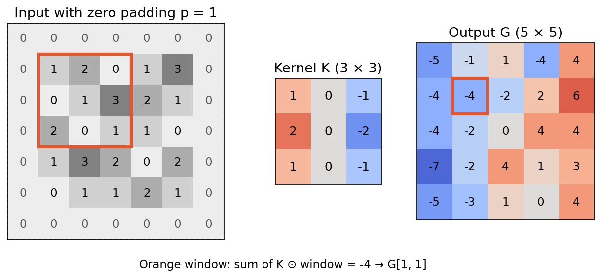
Two observations already matter for everything that follows. First, the same nine weights are used at every position: the operation is shift-invariant (also called space-invariant). Second, the operation is linear: filtering gives . Linear shift-invariant (LSI) operations are exactly the ones a convolution can express, which is why convolution is so central in signal processing.
Correlation versus convolution
Plain version. The formula above is technically cross-correlation. True convolution does the same thing with the kernel rotated by 180 degrees. For symmetric kernels the two agree; for asymmetric ones they differ.
Precise version. Mathematical convolution, written , is
The second form shows that convolution equals correlation with the flipped kernel . A clean way to see the difference is to filter a single bright pixel (an impulse). Correlation leaves a copy of the kernel rotated by 180 degrees; convolution leaves an exact copy of the kernel. That copy is the impulse response, and it is why signal processing prefers convolution: the output for any image is the sum of shifted, scaled impulse responses.
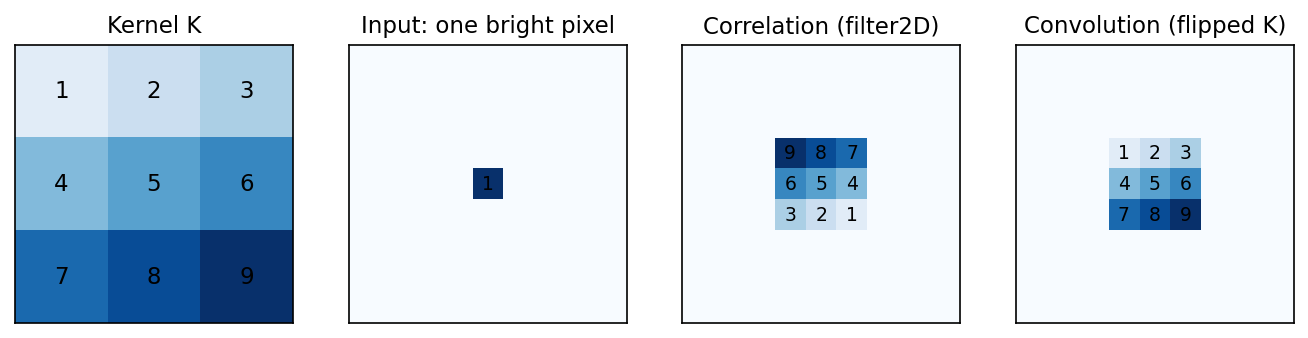
Convolution has algebraic properties that correlation lacks. It is commutative () and associative (), so two filters applied in a row equal one bigger filter. Applying a box blur twice, for instance, is a single kernel. Associativity also explains separable kernels: a Gaussian equals a column filter followed by a row filter, cutting the cost per pixel from to operations. The convolution theorem says convolution in space is multiplication in the Fourier domain; IP 04 develops that view.
Which libraries compute which?
| Library call | Computes | Default border |
|---|---|---|
cv2.filter2D | correlation [11] | reflect-101 (BORDER_DEFAULT) |
scipy.ndimage.correlate / convolve | correlation / convolution | reflect (edge sample repeated) |
scipy.signal.convolve2d | convolution | zero fill |
torch.nn.functional.conv2d, nn.Conv2d | correlation [31] | zero padding |
For hand-designed asymmetric kernels (Sobel, emboss, motion blur) the flip changes the sign or direction of the result, so flip deliberately when you need true convolution, for example with cv2.flip(K, -1). For learned kernels the distinction disappears: a network that “should” use the flipped kernel simply learns it. That is why deep-learning frameworks call their correlation “convolution” without harm.
Blur, edges and sharpening
Plain version. Positive weights that sum to one average neighbors and blur. Weights that sum to zero cancel flat regions and keep only changes, so they find edges. Adding a bit of “the image minus its blur” back to the image sharpens it.
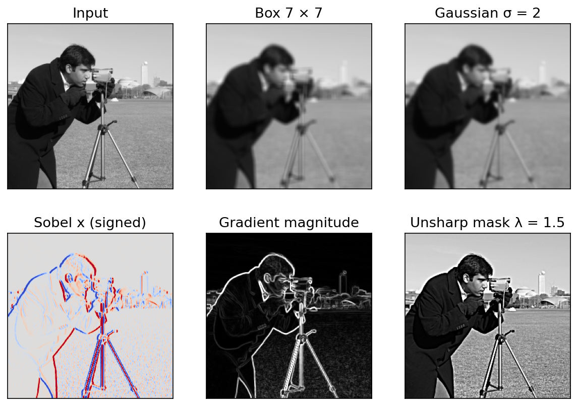
A box blur gives every neighbor equal weight; the version has nine entries of . A Gaussian blur samples
where (in pixels) sets the blur width and normalizes the weights to sum to one. Nearby pixels count more than distant ones, which avoids the blocky artifacts of a box. A practical rule is to use a kernel radius of about .
The sum of the weights tells you what happens in a flat region where every pixel equals : the output is . A blur with sum one preserves brightness; a kernel with sum two doubles it (and saturates an 8-bit image); a kernel with sum zero outputs zero.
The Sobel kernels estimate horizontal and vertical derivatives while smoothing in the orthogonal direction:
responds to intensity changes along , so it highlights vertical boundaries; highlights horizontal ones. The outputs , are signed: dark-to-light and light-to-dark edges have opposite signs. The gradient magnitude is a nonnegative edge strength, and is the edge orientation. The factorization shows that Sobel is separable: a smoothing column times a central difference.
The Laplacian kernel approximates ; it responds to thin lines and to both sides of an edge. Unsharp masking sharpens with
where is a Gaussian-blurred copy, is the high-frequency detail, and controls strength. Large amplifies noise and creates bright and dark halos along edges.
Try it: the kernel playground
Edit the kernel cells below and watch the output update. Start from Sobel x, then transpose it to detect horizontal edges instead of vertical ones. Make every weight of the blur preset larger and notice that flat regions brighten, exactly as the sum-of-weights rule predicts. Try the Laplacian and emboss presets and predict their kernel sums before you look.
The slider below compares a synthetic test image (a disc, a square, a checkerboard and stripes) with a Gaussian blur, . The fine stripes and the checkerboard disappear first because a blur is a low-pass filter: it removes fast intensity variations while leaving slow ones.
Code: from scratch, then OpenCV, SciPy and PyTorch
The loop below is the whole algorithm. Instead of looping over every pixel (slow in Python), it loops over the kernel taps and adds one shifted copy of the padded image per tap, which NumPy vectorizes. The script then checks that four libraries agree once you match the definition (correlation versus convolution) and the border rule. It needs numpy, scipy, opencv-python and torch.
Code · Python · 45 lines
import numpy as np
import cv2
import torch
import torch.nn.functional as F
from scipy import ndimage, signal

def correlate2d(img, K, mode="edge"):
    """Cross-correlation of a 2-D float image with an odd-sized kernel.
    mode is any np.pad mode: "constant" (zeros), "edge", "reflect", "wrap"."""
    kh, kw = K.shape
    ph, pw = kh // 2, kw // 2
    padded = np.pad(img, ((ph, ph), (pw, pw)), mode=mode)
    H, W = img.shape
    out = np.zeros((H, W), dtype=np.float64)
    for i in range(kh):              # loop over kernel taps, not pixels:
        for j in range(kw):          # each step adds one shifted copy of the image
            out += K[i, j] * padded[i:i + H, j:j + W]
    return out

def convolve2d(img, K, mode="edge"):
    return correlate2d(img, K[::-1, ::-1], mode)     # convolution = correlation with flipped K

rng = np.random.default_rng(0)
img = rng.random((32, 40))
K = rng.standard_normal((3, 5))                      # deliberately asymmetric

ours_corr = correlate2d(img, K, "reflect")
ours_conv = convolve2d(img, K, "reflect")
# OpenCV: filter2D computes correlation; BORDER_REFLECT_101 is np.pad's "reflect"
cv_corr = cv2.filter2D(img, cv2.CV_64F, K, borderType=cv2.BORDER_REFLECT_101)
# SciPy: ndimage.correlate / ndimage.convolve with mode="mirror" (= reflect-101)
sp_corr = ndimage.correlate(img, K, mode="mirror")
sp_conv = ndimage.convolve(img, K, mode="mirror")
# PyTorch: conv2d is correlation; pad first with the same rule
t = torch.tensor(img)[None, None]
t = F.pad(t, (2, 2, 1, 1), mode="reflect")
pt_corr = F.conv2d(t, torch.tensor(K)[None, None])[0, 0].numpy()

for name, a in [("OpenCV", cv_corr), ("SciPy", sp_corr), ("PyTorch", pt_corr)]:
    print(f"{name:8s} correlation matches:", np.allclose(ours_corr, a))
print("SciPy    convolution matches:", np.allclose(ours_conv, sp_conv))
print("conv == corr for this kernel?", np.allclose(ours_conv, ours_corr))
# zero padding: our convolution equals signal.convolve2d with mode="same"
same = signal.convolve2d(img, K, mode="same", boundary="fill")
print("zero-padded 'same' convolution matches:", np.allclose(convolve2d(img, K, "constant"), same))
All checks print True except conv == corr, which is False because the random kernel is asymmetric. Note the naming trap: NumPy’s "reflect" padding (dcb|abcd|cba, edge sample not repeated) is OpenCV’s BORDER_REFLECT_101 and SciPy’s "mirror", while SciPy’s "reflect" repeats the edge sample (dcba|abcd|dcba).
The second snippet shows the two bugs that cause most beginner frustration with real images: integer saturation and the kernel-sum rule.
Code · Python · 21 lines
import numpy as np
import cv2
from skimage import data

img_u8 = data.camera()                               # 512 x 512 uint8 test image
img = img_u8.astype(np.float32) / 255.0
sobel_x = np.array([[-1, 0, 1], [-2, 0, 2], [-1, 0, 1]], np.float32)

gx = cv2.filter2D(img, -1, sobel_x)                  # float in, float out: negatives kept
gy = cv2.filter2D(img, -1, sobel_x.T)
mag = np.hypot(gx, gy)
print("float Sobel x range:", gx.min().round(3), gx.max().round(3))

gx_u8 = cv2.filter2D(img_u8, -1, sobel_x)            # uint8 in, uint8 out: saturated
print("uint8 Sobel x range:", gx_u8.min(), gx_u8.max(),
      "| pixels clipped to 0:", f"{(gx_u8 == 0).mean():.0%}")

blur = cv2.GaussianBlur(img, (5, 5), 1.4)            # 5 x 5 Gaussian, sigma 1.4
print("mean brightness kept by blur:", np.isclose(img.mean(), blur.mean(), atol=1e-3))
K2 = 2 * np.ones((3, 3), np.float32) / 9             # weights sum to 2
print("mean after sum-2 kernel:", round(float(cv2.filter2D(img, -1, K2).mean() / img.mean()), 3))
In floating point the Sobel response ranges from about to . With uint8 input and output, every negative response is clipped to zero (more than half the pixels here), so all light-to-dark edges vanish. Always filter in float32 and convert back only for display.
Border handling
Plain version. Near the edge of the image, part of the kernel hangs outside. You must decide what values to pretend are there.
The common choices are: zero (constant) padding, which pretends the world outside is black; replicate, which repeats the edge pixel; reflect, which mirrors the image at its border; and wrap, which treats the image as periodic, as the discrete Fourier transform implicitly does. OpenCV’s default, BORDER_REFLECT_101, mirrors without repeating the edge pixel [11]. PyTorch’s nn.Conv2d uses zero padding unless you set padding_mode to 'reflect', 'replicate' or 'circular' [31].
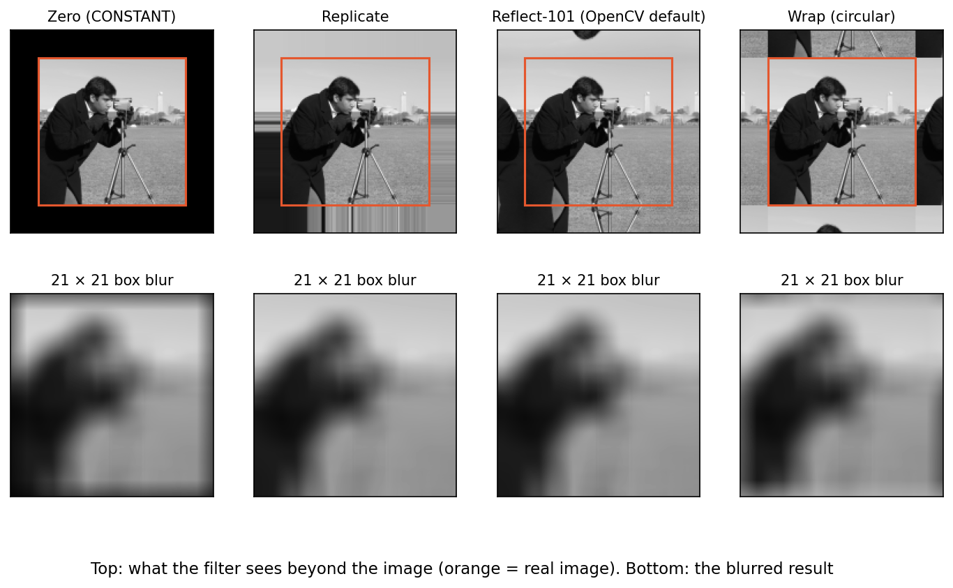
Zero padding darkens the borders of a blurred image because black pixels are averaged in. Wrap mixes the top of the image into the bottom. Replicate and reflect are usually the least visible choices for photographs. With small kernels the difference touches only a thin frame, but in a deep CNN every layer adds its own frame: after many zero-padded layers, a large fraction of the feature map has “seen” the artificial border, which lets networks infer absolute position from padding.
Part II · Convolutional neural networks
From a fixed filter to a learned layer
Plain version. A standard dense convolution learns filters spanning all input channels, each producing one output feature map. Grouped convolutions restrict that channel access.
Precise version. Let the input be (channels, height, width) and the weights with bias . A stride-one layer with zero padding computes
indexes output channels (filters), input channels, output positions and kernel taps; positions outside the image read the padding value. A nonlinearity such as ReLU is then applied element-wise. An RGB filter has three slices, one per color channel, and their responses are summed into a single output number per position: a filter does not produce three separate images.
Two structural assumptions are built into this formula:
- Local connectivity: each output depends only on a neighborhood, not on the whole image.
- Weight sharing (parameter sharing): the same is used at every position .
Together they are the CNN’s inductive bias, an assumption about which functions are likely. Its payoff is efficiency. A layer with , and has parameters, whatever the image size. A fully connected layer from a flattened image to just 32 numbers needs million weights, and it would have to learn the same edge detector separately at every position.
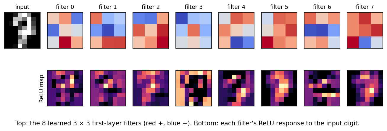
Goodfellow et al. [1] summarize the motivation as sparse interactions, parameter sharing and equivariance. Figure 5 shows what a tiny CNN learns in its first layer when trained on the digits dataset used in the classifier code later on. The learned filters look like oriented derivative and blob detectors: the network rediscovered Sobel-like kernels because they are useful, not because anyone told it to. Zeiler and Fergus [30] showed the same phenomenon at scale by visualizing the filters and feature maps of large ImageNet networks.
Padding, stride and dilation
Plain version. Padding controls what happens at the border and whether the output keeps its size. Stride skips positions to shrink the output. Dilation spreads the kernel taps apart to see farther without adding weights.
For input size (height or width), kernel size , padding on each side, stride and dilation , the output size is [12]
is the effective kernel size: dilation inserts gaps between taps. Three padding conventions have names: valid (, output shrinks by ), same ( for odd and , output keeps its size) and full (, every partial overlap counted, output grows by ). Stride two roughly halves each spatial dimension and is a common alternative to pooling for downsampling.
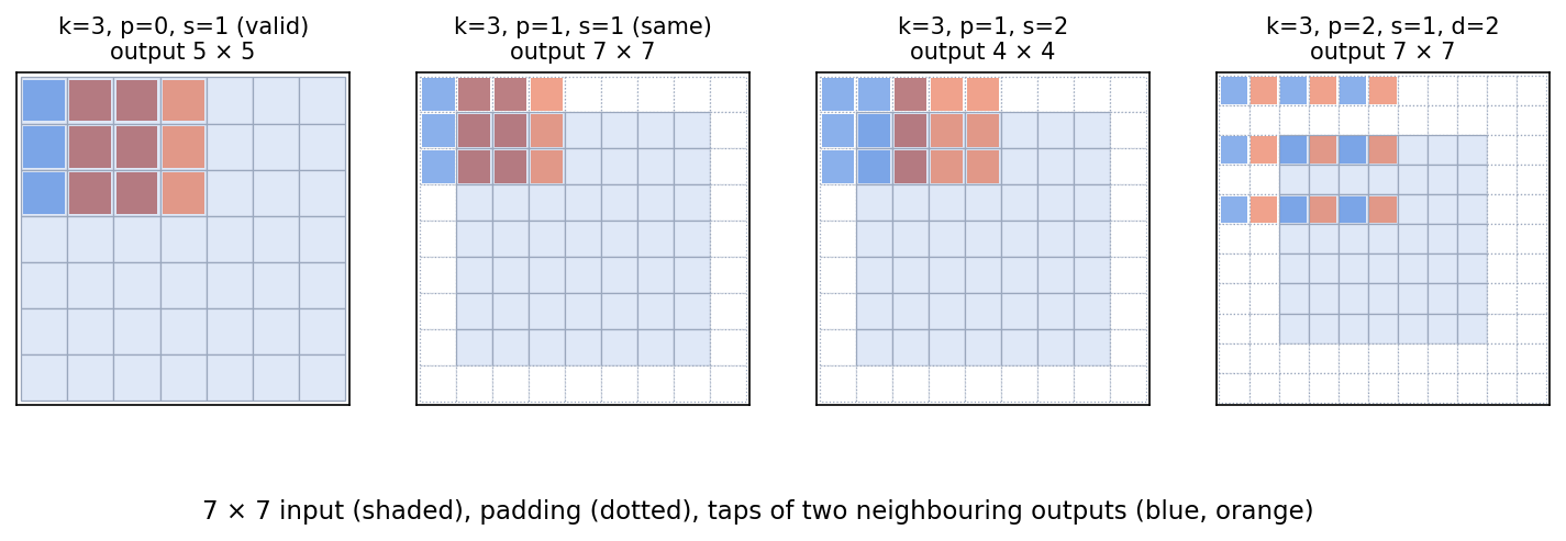
Dilated (atrous) convolutions were popularized for dense prediction by Yu and Koltun [18]: stacking layers with dilations 1, 2, 4, … grows the field of view exponentially while keeping full resolution. A single dilated layer sees only a sparse lattice of inputs, so dilations should be mixed with care to avoid “gridding” artifacts. A transposed convolution runs the forward map of a strided convolution backward to upsample; it reappears in the backpropagation section below. The convolution arithmetic guide by Dumoulin and Visin [12] has diagrams for every combination of these settings.
The snippet checks the formula against PyTorch, counts parameters, shows that a convolution is a per-pixel linear layer, and measures translation equivariance:
Code · Python · 35 lines
import torch
from torch import nn

def out_size(n, k, p=0, s=1, d=1):
    return (n + 2 * p - d * (k - 1) - 1) // s + 1

x = torch.randn(1, 3, 64, 64)                        # one RGB 64 x 64 image
for k, p, s, d in [(3, 1, 1, 1), (5, 2, 2, 1), (3, 2, 1, 2), (1, 0, 1, 1)]:
    conv = nn.Conv2d(3, 16, k, stride=s, padding=p, dilation=d)
    y = conv(x)
    n_params = sum(q.numel() for q in conv.parameters())
    assert y.shape[-1] == out_size(64, k, p, s, d)
    assert n_params == 16 * (3 * k * k + 1)
    print(f"k={k} p={p} s={s} d={d}: output {tuple(y.shape[1:])}, parameters {n_params}")

# A 1x1 convolution is the same linear layer applied at every pixel
conv1 = nn.Conv2d(16, 4, kernel_size=1)
lin = nn.Linear(16, 4)
lin.weight.data = conv1.weight.data[:, :, 0, 0].clone()
lin.bias.data = conv1.bias.data.clone()
z = torch.randn(2, 16, 8, 8)
same = torch.allclose(conv1(z), lin(z.permute(0, 2, 3, 1)).permute(0, 3, 1, 2), atol=1e-6)
print("1x1 conv == per-pixel Linear:", same)

# Translation equivariance away from borders (stride 1, no padding effects in the centre)
conv = nn.Conv2d(1, 4, 3, padding=1, bias=False)
img = torch.zeros(1, 1, 32, 32); img[..., 10:14, 8:12] = 1
shift = lambda t: torch.roll(t, shifts=(3, 5), dims=(-2, -1))
with torch.no_grad():
    a, b = conv(shift(img)), shift(conv(img))
print("shift then conv == conv then shift:", torch.allclose(a, b, atol=1e-6))
conv2 = nn.Conv2d(1, 4, 3, padding=1, stride=2, bias=False)
with torch.no_grad():
    y0, y1 = conv2(img), conv2(torch.roll(img, 1, dims=-1))   # shift by one pixel
print("stride 2, 1-pixel shift: max output change =", round((y0 - y1).abs().max().item(), 3))
It prints output shapes , , and with 448, 1216, 448 and 64 parameters, confirms the and equivariance checks, and shows that a one-pixel shift changes a stride-two output by a clearly nonzero amount; the exact value depends on the randomly initialized weights.
Channels and 1×1 convolutions
Plain version. Channels are the “what” dimension of a feature map; height and width are the “where”. A convolution mixes channels at each pixel without looking at neighbors.
A convolution with inputs and outputs multiplies the channel vector at every pixel by the same matrix, as the snippet verified. Lin et al.’s Network in Network [17] used this idea as a tiny per-pixel MLP and introduced global average pooling as a classifier head. GoogLeNet [16] used layers to reduce channels before expensive and branches, and ResNet’s bottleneck block [5] wraps a layer between a reduction and a expansion. In every case the motivation is the same: spatial filtering costs times more than channel mixing, so do the cheap part with layers and keep the expensive part narrow.
Pooling and downsampling
Plain version. Pooling summarizes each small block of a feature map by a single number, usually the maximum or the average. It shrinks the map and makes the representation less sensitive to small shifts.
Max pooling with a window and stride two keeps the largest value in each block: “was this feature present anywhere here?”. Average pooling keeps the mean. Global average pooling averages each channel over all positions, producing one number per channel regardless of input size, which is why modern classifiers can accept different image sizes. Pooling has no learnable parameters. Its gradient is simple: max pooling routes the whole upstream gradient to the winning input of each window; average pooling spreads it equally over the window.
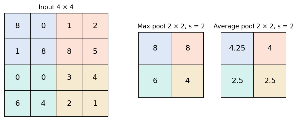
Downsampling, by pooling or by strided convolution, saves computation and enlarges later receptive fields, but it is also subsampling without a proper low-pass filter. High frequencies alias, and the output can change noticeably when the input moves by a single pixel, as the snippet above measured. Zhang [20] showed that inserting a small blur before subsampling (“anti-aliased” or “blur pooling”) makes standard CNNs measurably more shift-invariant: a neat case of a classical signal-processing rule fixing a deep network.
Equivariance is not invariance
Plain version. A stride-one convolution shifts with its input away from boundary effects. This equivariance does not make the prediction invariant to translation.
Let shift an image by pixels. Away from the borders, a stride-one convolution is translation-equivariant: . A classifier wants invariance: . CNNs get approximate invariance by stacking equivariant layers and then pooling, especially global average pooling, which discards position. Padding, strides, cropping and the finite image break exact equivariance. Rotation and scale equivariance are not built in; data augmentation or specially designed group-equivariant layers must supply them.
The distinction matters in practice. A detector must be equivariant: moving a person should move the predicted box. A classifier should be invariant: moving the person should not change the label. The same backbone serves both, with different heads.
Receptive field
Plain version. Early layers see small pieces of the image; deeper layers combine those pieces and see larger regions.
The receptive field of a unit is the set of input pixels that can influence it. Let be its width after layer , and the jump, the distance in input pixels between adjacent units of layer . Starting from , a layer with kernel size , dilation and stride gives
Three stacked stride-one layers see pixels, the same area as one layer but with instead of weights and three nonlinearities instead of one; this was the central design argument of VGG [15]. A stride-two layer doubles the jump, so every later layer grows the field twice as fast.
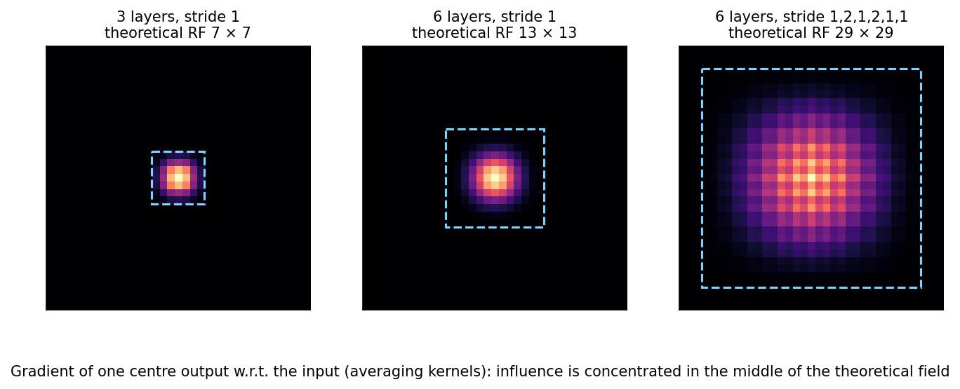
The theoretical field says which pixels could matter. Luo et al. [3] measured the effective receptive field via input gradients, as in Figure 8, and found that it is roughly Gaussian and occupies only a fraction of the theoretical field, growing like the square root of depth for uniform layers. Two practical lessons follow: a network may need more context than its theoretical field suggests, and downsampling, dilation and large kernels are ways to enlarge the effective field without unbounded depth.
Backpropagation through a convolution
Plain version. Kernel gradients combine inputs with upstream gradients. Input gradients use the transpose of the forward linear operator, with matching stride and padding conventions.
Precise version. Take one channel, no padding, stride one: . Let be the loss and the upstream gradient delivered by backpropagation, as in ML 02. Each weight is used at every output position, so by the chain rule its gradient sums over them:
That is a valid correlation of the input with , which is why weight sharing does not complicate training: shared weights simply accumulate gradients from every location. Each input pixel contributes to every output whose window covers it, at tap :
with taken as zero outside its range. This is a full convolution of with , equivalently a correlation of the zero-padded with the flipped kernel. It is exactly what a transposed convolution computes, which is how transposed convolutions got their name. Bias gradients are just per output channel. With multiple channels, the input gradient also sums over output channels, and the kernel gradient also sums over the batch.
Code · Python · 20 lines
import torch
import torch.nn.functional as F

torch.manual_seed(0)
X = torch.randn(1, 1, 6, 7, requires_grad=True)     # input
K = torch.randn(1, 1, 3, 3, requires_grad=True)     # kernel
Y = F.conv2d(X, K)                                   # 'valid' correlation: 4 x 5
G = torch.randn_like(Y)                              # pretend upstream gradient dL/dY
(Y * G).sum().backward()                             # so that dL/dY = G exactly

# 1) dL/dK: correlate the input with the upstream gradient
dK = F.conv2d(X.detach(), G)
# 2) dL/dX: 'full' convolution of G with K = correlation of zero-padded G with flipped K
dX = F.conv2d(F.pad(G, (2, 2, 2, 2)), K.detach().flip(-1, -2))
# 3) the same thing is what a transposed convolution computes
dX_t = F.conv_transpose2d(G, K.detach())

print("dL/dK matches autograd:", torch.allclose(dK, K.grad, atol=1e-5))
print("dL/dX matches autograd:", torch.allclose(dX, X.grad, atol=1e-5))
print("conv_transpose2d gives the same:", torch.allclose(dX_t, X.grad, atol=1e-5))
All three lines print True. The trick (Y * G).sum().backward() makes autograd use a chosen upstream gradient , a handy way to test any hand-derived backward pass.
Classic architectures in brief
Plain version. Every famous CNN is a stack of convolutions, nonlinearities and downsampling. What changed over the years was depth, how to keep deep stacks trainable, and how to spend computation wisely.
| Model (year) | Key idea | What it taught |
|---|---|---|
| LeNet-5 (1998) [13] | conv → subsample → conv → subsample → fully connected, trained end to end | Learned convolutional features beat hand-designed ones for digits |
| AlexNet (2012) [14] | Deeper and wider, ReLU, dropout, data augmentation, GPU training | Large labeled data plus GPUs made CNNs win ImageNet |
| VGG (2014) [15] | Only convolutions, 16–19 layers | Depth with small kernels is simple and effective |
| GoogLeNet / Inception (2014) [16] | Parallel , , branches with reductions | Multi-scale features at controlled cost |
| ResNet (2015) [5] | Residual connections , BatchNorm | Very deep networks (100+ layers) become trainable |
| U-Net (2015) [4] | Encoder–decoder with skip connections at each resolution | Dense, pixel-aligned outputs from few images |
| MobileNetV2 (2018) [7] | Depthwise-separable convolutions, inverted residuals, linear bottlenecks | Accurate models for phones |
| EfficientNet (2019) [8] | Compound scaling of depth, width and resolution | Scale dimensions together, not one at a time |
| ConvNeXt (2022) [9] | depthwise kernels, LayerNorm, inverted bottlenecks, transformer-era training | A modernized pure CNN competes with vision transformers |
The pattern from LeNet to ResNet is a steady increase in depth. AlexNet [14] showed that a deep CNN trained on ImageNet with GPUs, ReLU and dropout could beat traditional pipelines by a wide margin. VGG [15] argued for uniform stacks of layers, as computed in the receptive-field section. GoogLeNet [16] made width cheap with reductions. Then depth hit an optimization wall: plain networks with more layers had higher training error, which is not overfitting but a failure to optimize. ResNet [5] fixed it with identity shortcuts. DLCV 02 follows this line further, through training recipes, transfer learning and evaluation.
Residual blocks and normalization
Plain version. Instead of asking a block to compute the whole output, ask it to compute a correction to its input.
A residual block computes , where is typically two or three convolutions with normalization and ReLU. Its Jacobian is : even if contributes little, the identity path carries the signal forward and the gradient backward. If is the best a block can do, it can learn that easily, so adding blocks no longer hurts optimization. When the shape changes (more channels, stride two), the shortcut becomes a projection , usually a strided convolution.
Batch normalization [19] standardizes each channel using the batch mean and variance during training, then applies a learned scale and shift; at evaluation it uses running averages. It makes training faster and less sensitive to initialization, but it misbehaves with very small or correlated batches, where GroupNorm [6] (statistics over groups of channels within each sample) is more reliable. Always call model.eval() before validation so BatchNorm uses its running statistics.
Code · Python · 30 lines
import torch
from torch import nn

count = lambda m: sum(p.numel() for p in m.parameters())

C = 64
dense = nn.Conv2d(C, C, 3, padding=1, bias=False)
separable = nn.Sequential(
    nn.Conv2d(C, C, 3, padding=1, groups=C, bias=False),   # depthwise: one 3x3 per channel
    nn.Conv2d(C, C, 1, bias=False))                        # pointwise: mix channels
print("dense:", count(dense), "| depthwise+pointwise:", count(separable),
      "| ratio:", round(count(separable) / count(dense), 4), "vs 1/C + 1/9 =",
      round(1 / C + 1 / 9, 4))

class BasicBlock(nn.Module):
    """ResNet-style block: y = relu(x + F(x)), with a 1x1 projection when shapes change."""
    def __init__(self, c_in, c_out, stride=1):
        super().__init__()
        self.f = nn.Sequential(
            nn.Conv2d(c_in, c_out, 3, stride, 1, bias=False), nn.BatchNorm2d(c_out), nn.ReLU(),
            nn.Conv2d(c_out, c_out, 3, 1, 1, bias=False), nn.BatchNorm2d(c_out))
        self.proj = (nn.Identity() if stride == 1 and c_in == c_out else
                     nn.Sequential(nn.Conv2d(c_in, c_out, 1, stride, bias=False),
                                   nn.BatchNorm2d(c_out)))
    def forward(self, x):
        return torch.relu(self.proj(x) + self.f(x))

x = torch.randn(2, 64, 32, 32)
print("same shape :", tuple(BasicBlock(64, 64)(x).shape))
print("downsample :", tuple(BasicBlock(64, 128, stride=2)(x).shape))
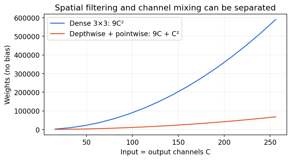
The output reports 36,864 weights for the dense layer against 4,672 for the separable pair, a ratio of 0.1267 that matches the formula below, and block outputs of shape and .
Efficient CNNs separate spatial filtering from channel mixing
Plain version. Looking around (spatial filtering) and combining features (channel mixing) need not happen in one expensive operation.
A dense convolution has weights. A depthwise convolution filters each channel separately ( weights, groups=C in PyTorch); a following pointwise convolution mixes channels ( weights). With ,
For and large this approaches .
MobileNetV2 [7] builds blocks that expand channels with a layer, filter with a depthwise , then project back with a linear (no ReLU) bottleneck, with a residual connection between the narrow ends. EfficientNet [8] scales depth, width and input resolution together with a single compound coefficient. ConvNeXt [9] started from a ResNet and applied, one at a time, design choices associated with vision transformers: patchify stem, depthwise kernels, inverted bottlenecks, fewer activations, LayerNorm, and longer training with heavy augmentation. The result matched Swin Transformers of similar size, evidence that much of the transformer advantage came from training recipes and macro-design rather than from attention alone.
Optional: ResNet (in the Paper guides). Read the original figure, evidence, design choices and limitations.
Code: a complete small-image classifier
This example needs torch, numpy and scikit-learn. It uses the bundled digits dataset, so no download or GPU is needed. A stratified split gives separate training, validation and test sets: validation picks the best epoch, and the test set is evaluated once at the end. It is a teaching baseline, not an ImageNet recipe.
Code · Python · 45 lines
import copy
import numpy as np
import torch
from torch import nn
from sklearn.datasets import load_digits
from sklearn.model_selection import train_test_split

torch.manual_seed(0)
torch.set_num_threads(1)
d = load_digits()
X = torch.tensor(d.images[:, None] / 16.0, dtype=torch.float32)
y = torch.tensor(d.target, dtype=torch.long)
train, test = train_test_split(np.arange(len(y)), test_size=.2,
                              stratify=d.target, random_state=0)
train, val = train_test_split(train, test_size=.2,
                             stratify=d.target[train], random_state=1)
model = nn.Sequential(
    nn.Conv2d(1, 16, 3, padding=1), nn.ReLU(),
    nn.Conv2d(16, 32, 3, padding=1), nn.ReLU(),
    nn.MaxPool2d(2),                     # B × 32 × 4 × 4
    nn.Flatten(), nn.Linear(32 * 4 * 4, 10),
)
opt = torch.optim.AdamW(model.parameters(), lr=1e-3, weight_decay=1e-4)
best_loss, best_state = float("inf"), None
for epoch in range(12):
    model.train()
    order = torch.tensor(train)[torch.randperm(len(train))]
    for idx in order.split(64):
        loss = nn.functional.cross_entropy(model(X[idx]), y[idx])
        opt.zero_grad()
        loss.backward()
        opt.step()
    model.eval()
    with torch.no_grad():
        val_loss = nn.functional.cross_entropy(model(X[val]), y[val]).item()
    if val_loss < best_loss:
        best_loss = val_loss
        best_state = copy.deepcopy(model.state_dict())
model.load_state_dict(best_state)
model.eval()
with torch.no_grad():
    accuracy = (model(X[test]).argmax(1) == y[test]).float().mean().item()
print("parameters:", sum(p.numel() for p in model.parameters()))
print("best validation loss:", round(best_loss, 4))
print("held-out accuracy:", round(accuracy, 4))
On our CPU run it reports 9,930 parameters and about 96% held-out accuracy (exact numbers vary slightly across PyTorch versions). Cross-entropy receives logits, with no softmax in front. The head flattens the map rather than global-average-pooling it, because on tiny digits the position of strokes carries information; for variable-size images, adaptive or global pooling gives a fixed-size head.
Inspect the errors, not just the score. Which digit pairs get confused? Does shifting every test digit by one pixel hurt? Compare against a parameter-matched MLP and a classical SVM, as in IP 13, before crediting every gain to convolution.
Modern view
Survey literature. Several reviews map the CNN landscape, each with a different emphasis. Gu et al. [23] (Pattern Recognition, 2018) organize CNN advances by component: convolution variants, pooling, activations, loss functions, regularization and optimization, followed by applications. Khan et al. [22] (Artificial Intelligence Review, 2020) propose a taxonomy of architectures by their main innovation: spatial exploitation (kernel sizes), depth, multi-path designs (shortcuts, Inception branches), width, feature-map exploitation (channel attention), and attention-based designs. Li et al. [21] (IEEE TNNLS, 2022) cover the history from LeNet onward, compare one-, two- and multi-dimensional convolutions, and survey lightweight networks and applications with rules of thumb for choosing hyperparameters. Alzubaidi et al. [2] (Journal of Big Data, 2021) give a broad, application-oriented review of deep learning centered on CNN architectures, with discussion of data scarcity, transfer learning and hardware. These surveys predate ConvNeXt, so read them as maps of the 2012–2020 era.
CNNs after transformers (2022–2026). Vision transformers (ML 05) prompted a re-examination of convolution, and the main finding is that the gap was smaller than early comparisons suggested:
- Modernized CNNs. ConvNeXt [9] showed that a carefully modernized ResNet matches Swin. ConvNeXt V2 [24] (CVPR 2023) added masked-autoencoder pretraining with sparse convolutions and a global response normalization layer, bringing self-supervised pretraining (see ML 06) to pure CNNs.
- Large kernels. RepLKNet [26] (CVPR 2022) used depthwise kernels as large as , with re-parameterized small kernels to ease optimization, to enlarge the effective receptive field. UniRepLKNet [27] (CVPR 2024) extended large-kernel design to audio, video, point clouds and time series.
- Dynamic and deformable convolution. InternImage [25] (CVPR 2023) scaled deformable convolution, whose sampling locations are predicted from the input, into a large foundation backbone for detection and segmentation.
- Scale. Smith et al. [29] (2023) pretrained NFNet CNNs on the large JFT-4B image dataset and found that their performance followed similar compute scaling trends to vision transformers under comparable budgets, arguing that compute and data, more than architecture, dominate at scale.
- Edge devices. MobileNetV4 [28] (ECCV 2024) designed blocks and a neural architecture search for good latency across CPUs, GPUs, DSPs and accelerators, an acknowledgment that parameter counts alone do not predict speed.
Where CNNs fit in 2026. Convolution remains a default for latency-constrained and on-device inference, for dense prediction at high resolution (restoration, segmentation, medical imaging, see DLCV 09), for small datasets where the locality bias helps, and as the stem or early stages of hybrid CNN–transformer models. Large vision foundation models are mostly transformer-based, but they frequently contain convolutions in their patch embeddings, upsampling decoders and diffusion U-Nets.
Open problems. Exact shift equivariance under downsampling (aliasing [20]); building rotation and scale symmetry in without heavy cost; understanding what the effective receptive field really needs to be for a task [3]; and fair comparison across architectures, which requires matching data, augmentation, resolution, schedule and compute before attributing a difference to convolution versus attention.
Key takeaways
- Convolution flips the kernel; correlation does not. Check the library convention when reproducing a filter.
- Kernel sums determine the response to constant input, but a sum of one alone does not imply smoothing.
- Learned filters share weights spatially; channel grouping determines which inputs each filter reads.
- Padding, stride and dilation determine shapes and sampling; downsampling may introduce aliasing.
- Translation equivariance differs from invariance; boundaries, stride and pooling affect the actual behavior.
- Separate spatial filtering, channel mixing and skip connections when comparing architectures; measure efficiency at matched budgets.
Exercises
- Design and verify. Write a kernel that detects only horizontal edges, and another that detects only diagonal edges running from top-left to bottom-right. Verify both in the kernel playground or with
cv2.filter2Don a synthetic image containing a horizontal, a vertical and a diagonal line.
Hint
A horizontal edge is a change along , so use (rows / / ). For a diagonal edge, put the derivative across the diagonal, for example . Its weights sum to zero, so flat regions give zero.
- Kernel sums. Why should a blur kernel’s weights sum to one? Predict, then check, what happens to a mid-gray
uint8image filtered with a kernel whose weights all equal , and what changes if you filter infloat32instead.
Hint
A flat region of value maps to . With sum two, a gray of 128 becomes 256, which saturates at 255 in uint8; every brighter-than-mid-gray region turns white. In float32 the values double without clipping, and you can rescale afterward.
- Composition. Show that applying a box blur twice equals one kernel, and write that kernel. Verify numerically away from the borders, and explain why the equality can fail at the borders.
Hint
By associativity, the combined kernel is the box convolved with itself: the outer product of with itself, divided by 81. At the border, the first pass already invented padding values, and the second pass pads that result; a single pass pads the original image instead, so the two differ in a frame of width two.
- Layer arithmetic. For a RGB input and a layer with 16 filters, , , : give the output shape and the number of parameters. Then compute after three layers with strides 1, 2, 1, and compare with all strides equal to one.
Hint
, so the output is with parameters. Receptive field: . All strides one gives .
- Gradient by hand. For a input and a kernel with valid correlation, write , then derive and in terms of . Check your formulas with the autograd trick from the backpropagation snippet.
Hint
. Then and (a correlation of with ). , the full convolution of with .
- Ablation on digits. In the classifier, replace
Flatten+Linear(512, 10)by global average pooling +Linear(32, 10). Compare parameter counts, validation loss and test accuracy, then evaluate both models on test digits shifted by one pixel. Explain the trade-off you observe.
Hint
nn.AdaptiveAvgPool2d(1) then nn.Flatten(). Pooling removes most head parameters and position information, which can help shift robustness but hurt on digits where stroke position matters. Keep everything else fixed, select on validation only, and report both accuracy and parameter count.
References
- I. Goodfellow, Y. Bengio and A. Courville, Deep Learning, MIT Press, 2016, ch. 9. Book
- L. Alzubaidi et al., “Review of deep learning: concepts, CNN architectures, challenges, applications, future directions,” Journal of Big Data, 2021. Review
- W. Luo, Y. Li, R. Urtasun and R. Zemel, “Understanding the Effective Receptive Field in Deep Convolutional Neural Networks,” NeurIPS, 2016. Paper
- O. Ronneberger, P. Fischer and T. Brox, “U-Net: Convolutional Networks for Biomedical Image Segmentation,” MICCAI, 2015. Paper
- K. He, X. Zhang, S. Ren and J. Sun, “Deep Residual Learning for Image Recognition,” CVPR, 2016. Paper
- Y. Wu and K. He, “Group Normalization,” ECCV, 2018. Paper
- M. Sandler et al., “MobileNetV2: Inverted Residuals and Linear Bottlenecks,” CVPR, 2018. Paper
- M. Tan and Q. Le, “EfficientNet: Rethinking Model Scaling for Convolutional Neural Networks,” ICML, 2019. Paper
- Z. Liu et al., “A ConvNet for the 2020s,” CVPR, 2022. Paper
- S. J. D. Prince, Understanding Deep Learning, MIT Press, 2023, ch. 10. Book and notebooks
- OpenCV, “Image Filtering” (
filter2D, border types), documentation, version 4.x. Documentation - V. Dumoulin and F. Visin, “A guide to convolution arithmetic for deep learning,” arXiv:1603.07285, 2016. arXiv
- Y. LeCun, L. Bottou, Y. Bengio and P. Haffner, “Gradient-based learning applied to document recognition,” Proceedings of the IEEE, 1998. DOI
- A. Krizhevsky, I. Sutskever and G. E. Hinton, “ImageNet Classification with Deep Convolutional Neural Networks,” NeurIPS, 2012. Paper
- K. Simonyan and A. Zisserman, “Very Deep Convolutional Networks for Large-Scale Image Recognition,” ICLR, 2015. arXiv
- C. Szegedy et al., “Going Deeper with Convolutions,” CVPR, 2015. arXiv
- M. Lin, Q. Chen and S. Yan, “Network In Network,” ICLR, 2014. arXiv
- F. Yu and V. Koltun, “Multi-Scale Context Aggregation by Dilated Convolutions,” ICLR, 2016. arXiv
- S. Ioffe and C. Szegedy, “Batch Normalization: Accelerating Deep Network Training by Reducing Internal Covariate Shift,” ICML, 2015. arXiv
- R. Zhang, “Making Convolutional Networks Shift-Invariant Again,” ICML, 2019. arXiv
- Z. Li, F. Liu, W. Yang, S. Peng and J. Zhou, “A Survey of Convolutional Neural Networks: Analysis, Applications, and Prospects,” IEEE Transactions on Neural Networks and Learning Systems, 2022. DOI
- A. Khan, A. Sohail, U. Zahoora and A. S. Qureshi, “A Survey of the Recent Architectures of Deep Convolutional Neural Networks,” Artificial Intelligence Review, 2020. arXiv
- J. Gu et al., “Recent Advances in Convolutional Neural Networks,” Pattern Recognition, 2018. arXiv
- S. Woo et al., “ConvNeXt V2: Co-designing and Scaling ConvNets with Masked Autoencoders,” CVPR, 2023. arXiv
- W. Wang et al., “InternImage: Exploring Large-Scale Vision Foundation Models with Deformable Convolutions,” CVPR, 2023. arXiv
- X. Ding et al., “Scaling Up Your Kernels to 31x31: Revisiting Large Kernel Design in CNNs” (RepLKNet), CVPR, 2022. arXiv
- X. Ding et al., “UniRepLKNet: A Universal Perception Large-Kernel ConvNet for Audio, Video, Point Cloud, Time-Series and Image Recognition,” CVPR, 2024. arXiv
- D. Qin et al., “MobileNetV4: Universal Models for the Mobile Ecosystem,” ECCV, 2024. arXiv
- S. L. Smith, A. Brock, L. Berrada and S. De, “ConvNets Match Vision Transformers at Scale,” arXiv:2310.16764, 2023. arXiv
- M. D. Zeiler and R. Fergus, “Visualizing and Understanding Convolutional Networks,” ECCV, 2014. arXiv
- PyTorch,
torch.nn.Conv2ddocumentation. Documentation
Check your understanding
This tutorial has 6 exercises. Can you solve them without opening the hints?
Go to the exercises ↑Next ML 04 · Recurrent and Recursive Networks · 27 min