ML 07 · Generative Models: Autoencoders, VAEs, GANs and Flows
Needs: ML 06 · Representation Learning and Self-Supervision
Navigate: this page and this track: Navigate: this page and this track
On this page
- What you’ll learn1 min
- The big picture1 min
- Modeling a distribution3 min
- Ordinary autoencoders: compression without a prior1 min
- VAEs: a latent-variable probability model5 min
- GANs: learning with an adversary5 min
- Normalizing flows: invertible transformations2 min
- Energy-based models1 min
- Autoregressive models, briefly1 min
- Diffusion models, briefly1 min
- The family map1 min
- Evaluating generative models4 min
- Modern view2 min
- Key takeaways1 min
- Exercises2 min
- Paper guides
- References
Machine Learning
Explore this chapter 2 interactive experiments
Move and widen a Gaussian posterior, then compute expected decoder loss and the exact KL penalty.
What you’ll learn
- Distinguish distribution modeling from label prediction.
- Compare likelihood-based models with implicit samplers.
- Derive the VAE bound and understand reparameterization.
- Explain adversarial training and invertible density transformations.
- Evaluate likelihood, realism, diversity and conditioning separately.
The big picture
A classifier asks, “What is in this image?” A generative model asks, “What kinds of images could occur?” If it learns a useful distribution, we can draw new samples, fill missing regions, compress data, detect unusual inputs, or condition generation on text, a class label or another image.
Learning a distribution is harder than learning a label. A label is one number; an image has thousands of pixels whose values depend on one another in complicated ways. Every family in this chapter is a different answer to the same engineering question: how do you represent a distribution over very high-dimensional data so that you can both train it from examples and sample from it afterwards?
This chapter uses the probabilistic viewpoint developed in Bishop and Bishop [1] and Prince [2]. The comparative review by Bond-Taylor et al. [3] organizes the same families along the trade-offs we will meet — training speed, sample quality, diversity, and whether a likelihood is available — and the flow review by Papamakarios et al. [4] is particularly helpful for distinguishing a learned distribution from a convenient sampling procedure. Diffusion and autoregressive models get their own chapters (ML 08 and ML 09) because their training and sampling deserve careful treatment; here we place them on the map.
Modeling a distribution
Plain version. Fit a probability model so that the observed examples look likely under it, then use the model to produce new examples that look like they came from the same source.
Maximum likelihood
Suppose the data are independent draws from an unknown distribution , and is a model with parameters . Maximum likelihood minimizes the average negative log-likelihood (NLL):
Here is the number of training examples and is the log-density the model assigns to example .
Why is this a sensible goal? As grows, the average approaches an expectation over the data distribution, and
is the Kullback–Leibler divergence, which is zero only when the two distributions agree, and is the entropy of the data, which does not depend on . So maximum likelihood is the same as minimizing the forward KL divergence from data to model.
The direction of the KL matters. The forward KL heavily punishes a model that assigns near-zero density where real data lives, so likelihood training is “mass-covering”: it prefers to spread probability over every mode, even if that means putting some probability between modes. Keep this in mind; we will see that GANs behave differently.
Densities, discrete pixels and bits per dimension
For continuous values, is a density, not the probability of observing exactly ; a density can exceed 1. Real images, however, store integers such as 0–255. Fitting a continuous density directly to integers is ill-posed: the model can place infinitely tall spikes on the integer grid and drive the likelihood to infinity. The standard fix is dequantization — add uniform noise in to each integer value before fitting a continuous density. Theis et al. [5] show that the continuous model’s log-likelihood on dequantized data is then a lower bound on the log-likelihood of a corresponding discrete model, which makes the numbers comparable across papers. Alternatively one uses a discrete likelihood directly (a softmax over 256 values, or a Bernoulli for binary pixels, as in our code below).
Image likelihoods are usually reported in bits per dimension:
Here is the number of stored values (height × width × channels). For a discrete model, is the negative log-probability in nats per image, and bpd is the ideal coding cost per stored value. A continuous density needs the dequantization convention too: if for 8-bit integers and independent uniform noise , its dequantization bound in bits per dimension is . The added 8 accounts for the volume of a quantization bin after rescaling. This is an upper bound on the discrete NLL per dimension, not an exact discrete likelihood [5]. State the units, noise distribution and any further change-of-variables correction before comparing scores.
Conditional and unconditional generation
A discriminative classifier models . A conditional generator models , where can be text, a class, a low-resolution image or observed pixels. Bayes’ rule links related quantities, but a classifier does not by itself provide an image sampler.
Conditioning also explains a familiar failure. Minimizing pixel MSE predicts the conditional mean . If an ambiguous input has several valid outputs — a gray-scale photo whose shirt could be red or blue — the mean blends them into a brownish average. A generative model instead tries to represent the whole distribution and sample one plausible answer at a time.
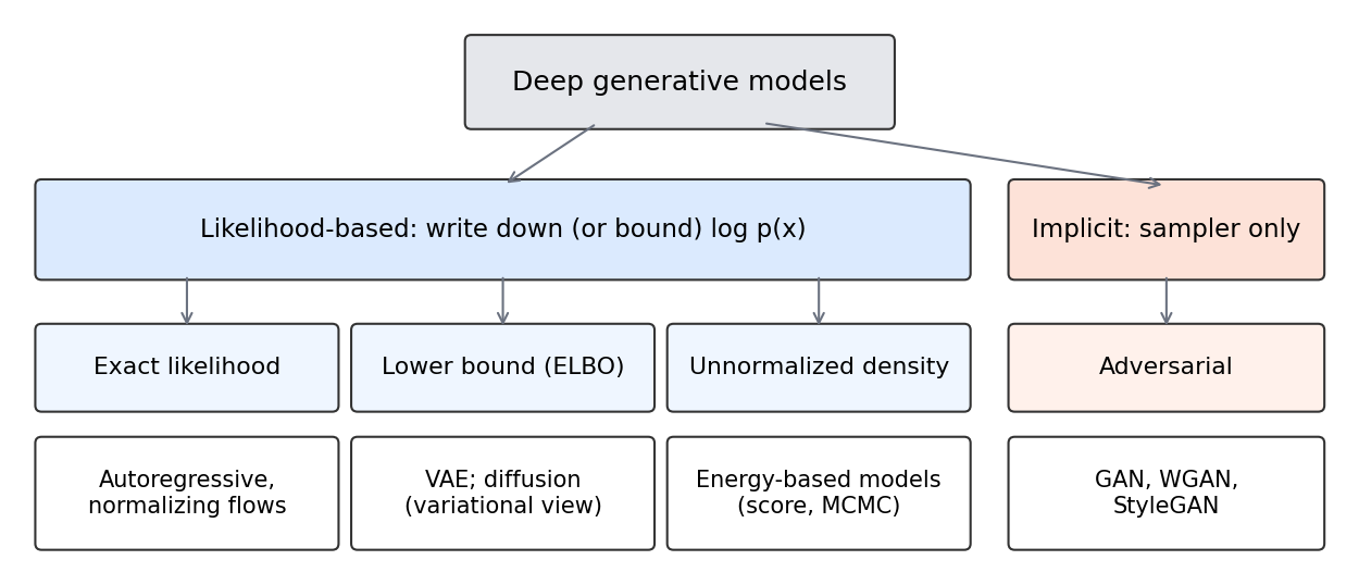
Two families: likelihood-based and implicit
Every model below needs two abilities: a way to train from data and a way to sample. They differ in whether they can evaluate .
- Likelihood-based (explicit) models write down a density, or a bound on it, and maximize it. Autoregressive models and normalizing flows give exact likelihoods; VAEs (and diffusion models, in their variational view) optimize a lower bound; energy-based models define a density only up to an unknown normalizing constant.
- Implicit models define a sampler — “push noise through a network” — without any formula for . GANs are the main example. Because there is no likelihood to maximize, they must be trained by comparing samples with data in some other way.
Ordinary autoencoders: compression without a prior
Plain version. Encode an example into a compact code and decode it back. That is excellent for compression and representation learning, but it does not by itself tell you how to invent new codes.
An encoder and decoder minimize a reconstruction loss such as . Autoencoders, their linear relatives (PCA, factor analysis) and their regularized variants are developed in ML 06A. The point for this chapter is narrow: an ordinary autoencoder places no requirement on where codes live. The training codes may occupy a thin, oddly shaped region of latent space. If you then sample and decode it, you may land in an empty region the decoder never saw, and get garbage. Excellent reconstruction therefore does not guarantee good unconditional generation.
A VAE fixes this by turning the autoencoder into a probability model with a prior over codes.
VAEs: a latent-variable probability model
Plain version. A VAE models observations through random latent codes and a decoder. Its encoder approximates the posterior over codes for each observation.
The model
Choose a prior over a latent vector , usually a standard Gaussian , and a decoder , a neural network that outputs the parameters of a distribution over images (Bernoulli probabilities for binary pixels, or Gaussian means). The model’s density over images is the marginal
Sampling is easy: draw , then draw . Evaluating is hard: the integral runs over every possible code, and the decoder is a nonlinear network, so there is no closed form. The true posterior is intractable for the same reason.
Deriving the evidence lower bound
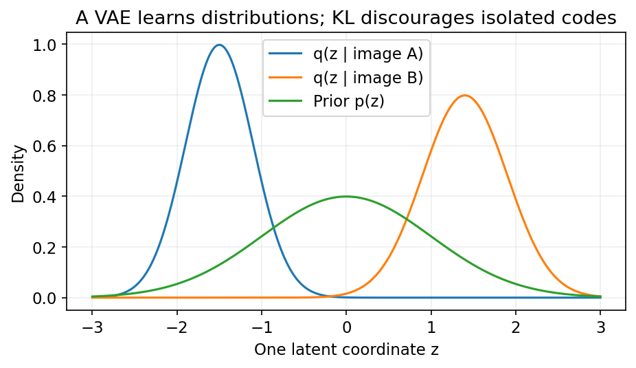
Kingma and Welling [6] introduce an encoder (or inference network) that approximates the posterior. Here is the derivation step by step. Since does not depend on , we can take its expectation under any distribution over without changing it:
The second line uses ; the third multiplies and divides by inside the log. Because a KL divergence is never negative, the first term is a lower bound on : the evidence lower bound (ELBO). The gap between the bound and the true log-likelihood is exactly the KL divergence between the approximate and true posteriors. A better encoder tightens the bound; a perfect one closes it.
Expanding gives the form used in code:
The first term rewards codes that let the decoder reproduce ; the second penalizes codes whose distribution wanders away from the prior. The same bound can be reached in one line with Jensen’s inequality (), but the decomposition above is more useful because it names the gap. Training maximizes the average ELBO over the data with respect to both and ; equivalently, it minimizes the negative ELBO.
For a diagonal Gaussian encoder and a standard Gaussian prior, the KL term has a closed form:
where and are the encoder’s mean and variance for latent coordinate . Each summand is zero exactly when and .
Reparameterization
The reconstruction term is an expectation over , and we need its gradient with respect to . Sampling is not differentiable as written: a random draw is a black box. The reparameterization trick [6] moves the randomness into a fixed noise variable:
Here is elementwise multiplication. Now is a deterministic, differentiable function of and an independent , so ordinary backpropagation gives low-variance gradient estimates through and . In code, the encoder predicts logvar and uses exp(.5 * logvar) as the standard deviation, which guarantees positivity without constraints.
Code: a small VAE for binary digits
This complete CPU example uses scikit-learn’s bundled 8 × 8 digits, binarized so that a Bernoulli decoder is a stated likelihood model. Reconstruction is summed over pixels and KL over latent dimensions, then both are averaged over examples; silently averaging only one term would change their balance.
Code · Python · 39 lines
import torch
from torch import nn
from torch.nn import functional as F
from sklearn.datasets import load_digits
from sklearn.model_selection import train_test_split

torch.manual_seed(0)
torch.set_num_threads(1)
d = load_digits()
train, test = train_test_split(d.data, test_size=.2, random_state=0,
                              stratify=d.target)
X = torch.tensor((train > 8).astype("float32"))
Xt = torch.tensor((test > 8).astype("float32"))
enc = nn.Sequential(nn.Linear(64, 64), nn.ReLU(), nn.Linear(64, 16))
dec = nn.Sequential(nn.Linear(8, 64), nn.ReLU(), nn.Linear(64, 64))
opt = torch.optim.Adam(list(enc.parameters()) + list(dec.parameters()), lr=.002)

def terms(x):
    mu, logvar = enc(x).chunk(2, dim=-1)
    z = mu + (.5*logvar).exp() * torch.randn_like(mu)
    recon = F.binary_cross_entropy_with_logits(dec(z), x, reduction="none").sum(1)
    kl = .5*(mu.square() + logvar.exp() - logvar - 1).sum(1)
    return recon, kl

for step in range(400):
    x = X[torch.randint(len(X), (64,))]
    recon, kl = terms(x)
    loss = (recon + kl).mean()
    opt.zero_grad()
    loss.backward()
    opt.step()
enc.eval(); dec.eval()
with torch.no_grad():
    recon, kl = terms(Xt)
    samples = dec(torch.randn(4, 8)).sigmoid().reshape(4, 8, 8)
    print("test negative ELBO estimate:", round((recon + kl).mean().item(), 3))
    print("reconstruction / KL:", round(recon.mean().item(), 3),
          round(kl.mean().item(), 3))
    print("sample probability maps:", tuple(samples.shape))
On our machine it prints a test negative ELBO of about 20.5 nats per image, split into roughly 17.0 nats of reconstruction and 3.5 nats of KL. Since the bound is a lower bound on log-likelihood, 20.5 nats is an upper bound on the test NLL. The output maps are Bernoulli probabilities; to obtain binary samples, draw each pixel with those probabilities. The test estimate is stochastic, so average several latent draws for a more stable number. No test-based checkpoint selection happens here.
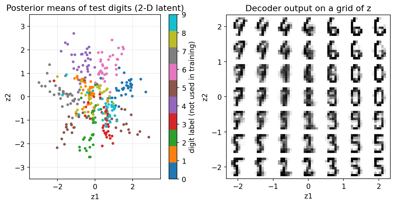
Figure 3 shows what a VAE with only a two-dimensional latent space learns on the same data (trained longer by the figure script). Even though labels are never used, digits of the same class land near each other, and decoding a regular grid of values produces smooth transitions between digit shapes. This is the property an ordinary autoencoder lacks: every point near the prior’s bulk decodes to something digit-like.
Posterior collapse, β-VAE and deeper VAEs
If the decoder is very powerful (for example, an autoregressive decoder that can model pixels on its own), the cheapest way to raise the ELBO may be to ignore entirely: set so the KL term is zero, and let the decoder do all the work. This is posterior collapse. Bowman et al. [7] observed it when training VAEs on text and proposed KL annealing: start with a small weight on the KL term and raise it to 1 during training, so the model learns to use the code before the penalty bites. Monitoring the KL per latent dimension is the simplest diagnostic — dimensions with KL near zero carry no information.
Higgins et al. [8] go the other way: the β-VAE multiplies the KL term by , pressuring the model toward a more factorized, “disentangled” code at the cost of reconstruction. Be precise about what this means: with the objective is no longer the ELBO, so the value is not a bound on , and Kingma and Welling’s tutorial review [9] discusses this and many other variants. Finally, single-layer VAEs with factorized Gaussians tend to produce blurry images, partly because the Gaussian decoder averages over uncertainty. Hierarchical VAEs stack several layers of latent variables; NVAE [10] showed that a carefully engineered deep hierarchy with stabilizing regularization can produce sharp samples on natural images up to 256 × 256 pixels.
Optional: VAE (in the Paper guides). Read the original figure, evidence, design choices and limitations.
GANs: learning with an adversary
Plain version. A generator learns to fool a discriminator that separates generated samples from data. This competing objective can improve samples, but training can be unstable.
The minimax game
Let map noise to samples , whose distribution we call . Let be the discriminator’s estimated probability that is real. The original GAN objective of Goodfellow et al. [11] is
The discriminator maximizes : it is ordinary binary cross-entropy with real data labeled 1 and fakes labeled 0. The generator minimizes : it wants to be large.
What the game minimizes
For a fixed generator, write as an integral over : . For each separately, the function with is maximized at (set the derivative to zero). So the optimal discriminator is
It is the probability that a point came from the data rather than the generator, if both were equally likely a priori. Substituting back in and adding and subtracting gives
where with is the Jensen–Shannon divergence. So, with a perfect discriminator, the generator minimizes a symmetric divergence between data and model, and the global optimum is , where everywhere [11]. Notice that no likelihood was ever computed: the discriminator acts as a learned, adaptive test of “does this look like the data?”
The non-saturating loss and how to implement it
Early in training the generator is poor, , and is flat, so the generator’s gradient vanishes. In practice the generator instead minimizes , the non-saturating loss proposed in the same paper [11], which has strong gradients precisely when the generator is losing. It has the same fixed point but different dynamics.
Updates alternate. When updating , detach generated samples so no gradient reaches ; when updating , let gradients flow through into but step only ‘s optimizer. Using logits with binary_cross_entropy_with_logits is numerically safer than applying a sigmoid and then a log.
Code: a GAN on eight Gaussians
The classic test bed for mode coverage is a ring of eight tight Gaussian clusters in 2-D. It is small enough to train on a CPU in under a minute, and you can see whether every mode is covered.
Code · Python · 42 lines
import math
import torch
from torch import nn
from torch.nn import functional as F

torch.manual_seed(0)
torch.set_num_threads(1)
angles = torch.arange(8) * (2 * math.pi / 8)
centers = 2.0 * torch.stack([angles.cos(), angles.sin()], dim=1)

def sample_data(n):
    idx = torch.randint(8, (n,))
    return centers[idx] + 0.05 * torch.randn(n, 2)

def mlp(i, o):
    return nn.Sequential(nn.Linear(i, 128), nn.ReLU(),
                         nn.Linear(128, 128), nn.ReLU(), nn.Linear(128, o))

G, D = mlp(8, 2), mlp(2, 1)
opt_g = torch.optim.Adam(G.parameters(), lr=1e-3, betas=(.5, .999))
opt_d = torch.optim.Adam(D.parameters(), lr=1e-3, betas=(.5, .999))
for step in range(3000):
    real = sample_data(256)
    fake = G(torch.randn(256, 8))
    # Discriminator: logits, real -> 1, fake -> 0; detach so G is untouched.
    d_loss = (F.binary_cross_entropy_with_logits(D(real), torch.ones(256, 1))
              + F.binary_cross_entropy_with_logits(D(fake.detach()),
                                                   torch.zeros(256, 1)))
    opt_d.zero_grad(); d_loss.backward(); opt_d.step()
    # Generator: non-saturating loss -log D(G(z)).
    g_loss = F.binary_cross_entropy_with_logits(D(fake), torch.ones(256, 1))
    opt_g.zero_grad(); g_loss.backward(); opt_g.step()

with torch.no_grad():
    x = G(torch.randn(5000, 8))
    dist = torch.cdist(x, centers)
    nearest = dist.min(1)
    good = nearest.values < 0.15          # within 3 std of some mode
    counts = torch.bincount(nearest.indices[good], minlength=8)
print("fraction near a mode:", round(good.float().mean().item(), 3))
print("modes with >= 1% of samples:", int((counts >= 50).sum()))
print("samples per mode:", counts.tolist())
It prints:
Code · 3 lines
fraction near a mode: 0.896
modes with >= 1% of samples: 7
samples per mode: [590, 14, 710, 276, 651, 731, 863, 646]
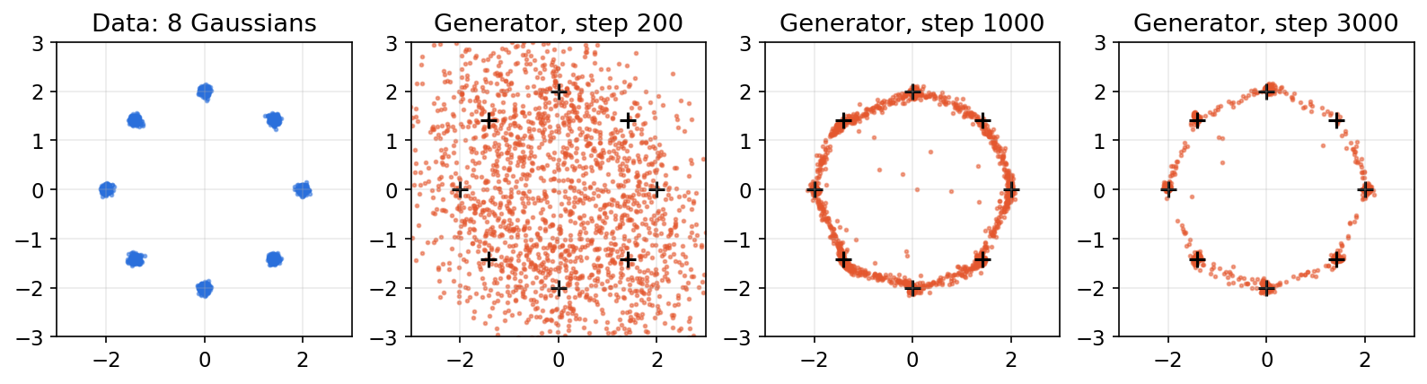
About 90% of samples land on a mode, but the mode at 45° receives only 14 of 5,000 samples and another is under-represented. That is partial mode collapse caught in the act. Figure 4 shows the generator’s journey: an unstructured cloud early on, a ring that covers every mode but also the space between them, and finally sharper clusters with one mode nearly abandoned. Exact numbers depend on the seed and library version; the qualitative picture is typical.
Mode collapse and why it happens
Mode collapse occurs when the generator produces too few kinds of output. The generator is rewarded for samples the current discriminator accepts, not for diversity. If it finds one region the discriminator likes, it can pile samples there; the discriminator then learns to reject that region, the generator hops to another, and the pair can chase each other around instead of converging. Unlike maximum likelihood, nothing in the per-sample generator loss directly punishes missing a mode. Salimans et al. [12] proposed early remedies such as feature matching and minibatch discrimination, which let the discriminator look at statistics of a whole batch so that a lack of diversity becomes detectable.
A collection of sharp, convincing images can therefore still cover only a small part of the data distribution. Always measure coverage separately from quality — we return to this under evaluation.
Wasserstein GANs
When and live on thin, non-overlapping sets (as images do in pixel space), the JSD is stuck at its maximum and provides no useful gradient about how far apart they are. Arjovsky et al. [13] proposed the Wasserstein-1 (earth mover’s) distance instead: the minimum cost of moving probability mass from one distribution to the other. Its dual form, from the Kantorovich–Rubinstein theorem, is
where the supremum is over all 1-Lipschitz functions (functions whose output changes by at most when the input changes from to ). The network is now called a critic: it outputs an unbounded score, not a probability. The Wasserstein distance shrinks smoothly as the generator’s samples move toward the data, even when the supports do not overlap.
The hard part is enforcing the Lipschitz constraint. The original WGAN clips every critic weight to a small interval, which is crude and can make the critic too simple. WGAN-GP [14] instead adds a gradient penalty
where is drawn uniformly on straight lines between pairs of real and generated samples and is a weight (the paper uses 10). Two other widely used stabilizers act on the discriminator directly: spectral normalization [15] divides each weight matrix by its largest singular value, bounding the Lipschitz constant layer by layer, and the R1 penalty analyzed by Mescheder et al. [16] penalizes on real data, which they show gives local convergence where unregularized GAN training can oscillate.
Architectures and where GANs are used now
StyleGAN [17] illustrates how architecture matters as much as the loss: it maps noise to an intermediate latent space and injects that “style” at every resolution, giving controllable, high-quality face synthesis. GANs sample with a single generator pass, which makes them fast at inference. Adversarial losses also appear as components of other systems — for example, inside image tokenizers trained to reconstruct sharp detail. That does not make every model using such a tokenizer a GAN generator; the distribution may be modeled by something else entirely.
Optional: GAN (in the Paper guides). Read the original figure, evidence, design choices and limitations.
Normalizing flows: invertible transformations
Plain version. A normalizing flow transforms a simple density through invertible maps. Tracking each map’s volume change makes the modeled density computable.
Change of variables
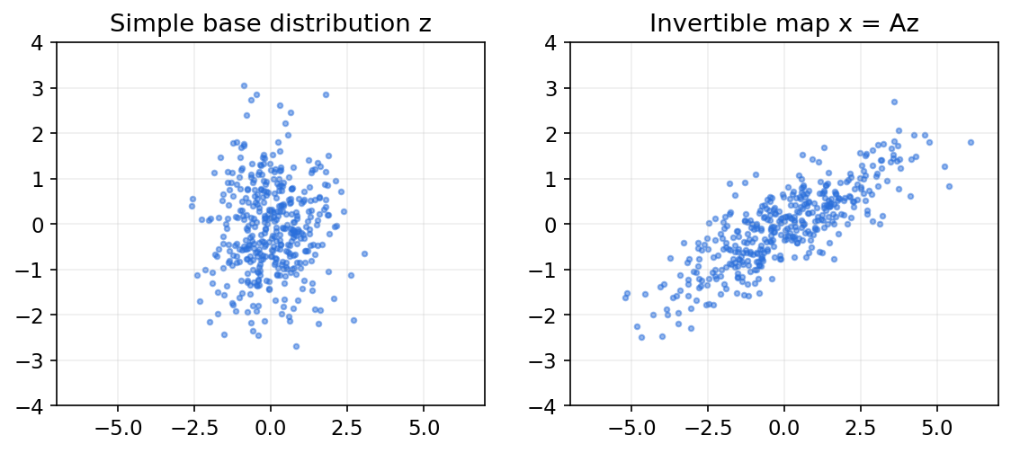
Let be a simple base distribution and an invertible, differentiable map with the same dimension. Then
is the Jacobian matrix of the map, and its determinant measures how much the map scales a small volume around . Probability mass is conserved, so if a region is stretched to twice its volume, its density must halve. In one dimension, doubles every interval and adds to the log density. A composition simply adds up the log-determinants of the steps.
Coupling layers
The formula is exact, but a general determinant costs — hopeless for images. Flow layers are designed so that the Jacobian is triangular, whose determinant is just the product of the diagonal. The affine coupling layer of RealNVP [18] splits into two halves and computes
where and are arbitrary neural networks. The Jacobian is block-triangular with the identity on the first block and on the second, so . The inverse is just as cheap: . Crucially, and never need to be inverted, so they can be as complex as you like. Stacking layers with alternating splits lets every coordinate be transformed. Glow [19] added learned invertible 1 × 1 convolutions as a generalized channel permutation between coupling layers.
Code: verify a coupling layer’s log-determinant
The snippet below builds one affine coupling layer and checks its cheap log-determinant against the full Jacobian computed by autograd.
Code · Python · 40 lines
import torch
from torch import nn

torch.manual_seed(0)

class AffineCoupling(nn.Module):
    """RealNVP-style layer: keep x1, scale-and-shift x2 using x1."""
    def __init__(self, dim, hidden=32):
        super().__init__()
        self.d = dim // 2
        self.net = nn.Sequential(nn.Linear(self.d, hidden), nn.Tanh(),
                                 nn.Linear(hidden, 2 * (dim - self.d)))

    def forward(self, x):
        x1, x2 = x[..., :self.d], x[..., self.d:]
        s, t = self.net(x1).chunk(2, dim=-1)
        s = torch.tanh(s)                       # keep scales moderate
        y2 = x2 * s.exp() + t
        return torch.cat([x1, y2], -1), s.sum(-1)   # output, log|det J|

    def inverse(self, y):
        y1, y2 = y[..., :self.d], y[..., self.d:]
        s, t = self.net(y1).chunk(2, dim=-1)
        s = torch.tanh(s)
        return torch.cat([y1, (y2 - t) * (-s).exp()], -1)

layer = AffineCoupling(4)
x = torch.randn(4)
y, logdet = layer(x)
J = torch.autograd.functional.jacobian(lambda v: layer(v)[0], x)
print("log|det J| from layer:   ", round(logdet.item(), 5))
print("log|det J| from autograd:", round(torch.linalg.slogdet(J)[1].item(), 5))
print("upper-right block is zero:", bool(torch.allclose(J[:2, 2:], torch.zeros(2, 2))))
print("inverse error:", (layer.inverse(y) - x).abs().max().item() < 1e-6)

# Log density of y under a standard-normal base after one layer:
base = torch.distributions.Normal(0., 1.)
z = layer.inverse(y)
log_px = base.log_prob(z).sum() - layer(z)[1]
print("log p(y):", round(log_px.item(), 4))
Both log-determinants print 0.14867, the upper-right Jacobian block is exactly zero (the triangular structure), and the inverse recovers the input. The last line is the change-of-variables formula in action. Training a flow simply maximizes this log p over data with a stack of such layers.
Strengths, limits and continuous flows
Flows give exact likelihoods, exact inversion (useful for editing and for mapping data to a well-behaved latent space) and one-pass sampling. The price is architectural: every layer must be invertible with a cheap determinant, and the latent must have the same dimension as the data, which wastes capacity on representing noise in all pixel directions. Rezende and Mohamed [20] introduced flows as a way to make the approximate posterior of a VAE more flexible, which shows that the same tool serves inference as well as generation.
Continuous normalizing flows replace a discrete stack by an ordinary differential equation . Neural ODEs [21] showed that the log-density then evolves through the divergence (trace of the Jacobian) of rather than a determinant, which removes the architectural restriction but makes likelihood evaluation require an ODE solve. Flow matching [22], covered in ML 08, trains such a vector field by simple regression instead of maximum likelihood. The word “flow” therefore refers to related transformations, but the training objective need not be likelihood.
Energy-based models
Plain version. Instead of describing how to generate an image, give every possible image a score — an “energy” — where low energy means “looks real.” Probability is high wherever energy is low.
An energy-based model (EBM) defines
where is any network that outputs a scalar and is the partition function that makes the density integrate to one. EBMs are extremely flexible — any architecture works — but is intractable in high dimensions, so neither the likelihood nor exact samples are directly available. Goodfellow, Bengio and Courville [23] cover the classical tools (the partition-function chapter and approximate inference), and Song and Kingma [24] survey modern training routes: maximum likelihood with MCMC samples (for example, Langevin dynamics), score matching, which fits and thereby never needs , and noise-contrastive methods. Score matching is the bridge to diffusion models.
Autoregressive models, briefly
Plain version. Generate an image one piece at a time, each piece conditioned on everything generated so far, like writing a sentence word by word.
The chain rule of probability is exact for any ordering of the elements of :
Each factor is an ordinary classification or regression problem, so training is simple, stable maximum likelihood with an exact likelihood. PixelRNN and PixelCNN [25] modeled raw pixels this way with a 256-way softmax per subpixel. The drawback is sequential sampling: network evaluations for elements. Modern systems instead predict compressed tokens, groups of tokens or whole scales at once. ML 09 develops this family in detail.
Diffusion models, briefly
Plain version. Teach a network to remove a little noise from a noisy image. Then start from pure noise and apply the denoiser many times, slowly sculpting an image.
A diffusion model defines a fixed forward process that gradually adds Gaussian noise to data until nothing but noise remains, and learns a reverse process that undoes it step by step. Ho et al. [26] showed that training reduces, up to weighting, to predicting the noise that was added — a simple regression — and that the objective is a reweighted variational bound, which is why the taxonomy in Figure 1 lists diffusion next to the VAE. The connection to score matching (see the energy-based models section) gives a second, equivalent view. The survey by Yang et al. [27] maps the many variants. Diffusion and flow matching now dominate high-quality image generation and are the subject of ML 08.
The family map
| Family | Basic training signal | Sampling mechanism | Likelihood | Main qualification |
|---|---|---|---|---|
| VAE | Variational bound (ELBO) | Sample latent, then decoder (one pass) | Lower bound | Bound depends on approximate inference; samples can be blurry |
| GAN | Adversarial discrimination | Generator pass (one pass) | None | Unstable game; mode collapse |
| Normalizing flow | Change-of-variables likelihood | Invertible transform (one pass) | Exact | Invertibility and same-dimension constraints |
| Autoregressive | Conditional likelihoods | Sequential conditional sampling | Exact | Generation dependencies can be costly |
| Diffusion | Denoising/score objectives | Reverse noise process (many steps) | Bound or ODE-based | Quality depends on model and sampler |
| Flow matching | Velocity regression | Integrate learned vector field | Needs extra computation | Integration cost |
| Energy-based | Energy learning (MCMC, score matching) | Often iterative sampling | Unnormalized | Normalization and mixing can be hard |
Bond-Taylor et al. [3] summarize these trade-offs as a triangle that is hard to satisfy all at once: fast sampling, high sample quality, and good mode coverage. GANs are fast and sharp but can miss modes; likelihood models cover modes but were historically slower or blurrier; diffusion models reach high quality and coverage at the cost of many sampling steps. This table is a teaching synthesis, not an exclusive taxonomy. Real models combine families: a VAE compresses an image, a transformer models its latent distribution, and a diffusion objective trains that transformer.
Evaluating generative models
Plain version. A generator can be good in different ways: it can assign high probability to real data, make individually convincing samples, cover all the variety in the data, or follow its conditioning. No single number captures all of these, so use several measures and know what each misses.
Theis et al. [5] made this point sharply: average log-likelihood, sample quality and older proxies such as Parzen-window estimates can be largely independent of one another in high dimensions. A model can have excellent likelihood and poor samples, or the reverse. Evaluate against the purpose you have in mind.
Likelihood
For likelihood-based models, held-out NLL (or bits per dimension) is principled and comparable when dequantization and preprocessing match. It cannot be computed for GANs. And a high likelihood need not mean reliable out-of-distribution detection: Nalisnick et al. [28] found that flows, VAEs and PixelCNNs trained on CIFAR-10 can assign higher likelihood to the unrelated SVHN digit images, because likelihood is dominated by low-level statistics such as smoothness rather than semantic content.
Inception Score
Salimans et al. [12] proposed the Inception Score (IS). Feed each generated image to a pretrained ImageNet classifier (Inception-v3) to get a label distribution , and let be the average over samples. Then
IS is high when each image is confidently classified ( peaked) and the set covers many classes ( spread out). It never looks at real data, so it cannot tell whether samples resemble your dataset, and it is meaningful only for ImageNet-like content.
Fréchet Inception Distance
The Fréchet Inception Distance (FID) of Heusel et al. [29] compares real and generated images in a feature space. Extract Inception-v3 features for both sets, fit a Gaussian to each — means and covariances — and compute the Fréchet distance between the Gaussians:
Lower is better. FID uses real data and is sensitive to both quality and diversity, which made it the standard metric. But it is not an image-by-image truth measure: it depends on the feature extractor, image resizing, and especially the number of samples (it is biased for finite sets, so compare FIDs only with equal sample counts), and it folds quality and coverage into one number.
Precision and recall
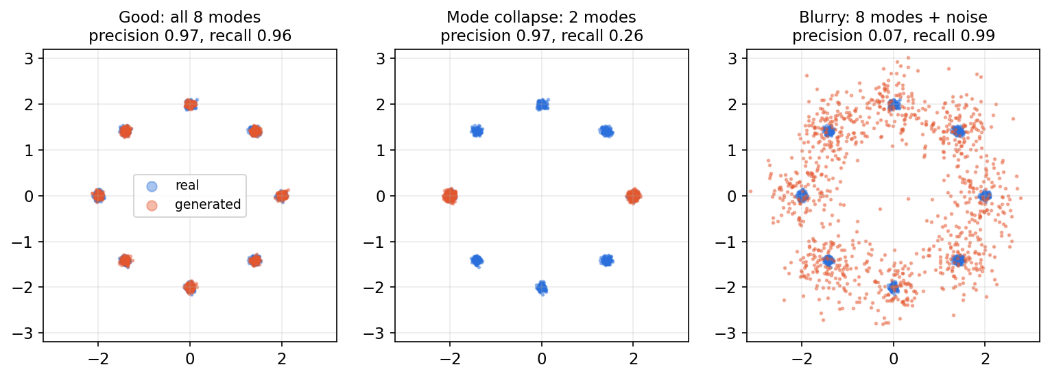
To separate the two, Sajjadi et al. [30] defined precision and recall for distributions: precision asks what fraction of generated samples fall where real data lives (quality), recall asks what fraction of the real distribution the generator covers (diversity). Kynkäänniemi et al. [31] gave a simple, robust estimator that we implement below. Approximate each set’s manifold by a union of balls around its points, with each ball’s radius equal to the distance to the point’s -th nearest neighbor in the same set. Then
- precision = fraction of generated samples inside some real sample’s ball;
- recall = fraction of real samples inside some generated sample’s ball.
On images, the points are deep features rather than pixels. On our 2-D ring we can use coordinates directly:
Code · Python · 30 lines
import numpy as np

rng = np.random.default_rng(0)
angles = np.arange(8) * 2 * np.pi / 8
centers = 2 * np.stack([np.cos(angles), np.sin(angles)], 1)

def ring(n, modes):
    idx = rng.choice(modes, n)
    return centers[idx] + .05 * rng.standard_normal((n, 2))

def knn_radius(a, k):
    d = np.linalg.norm(a[:, None] - a[None], axis=-1)
    return np.sort(d, axis=1)[:, k]          # column 0 is the point itself

def coverage(query, ref, k=3):
    """Fraction of query points inside some reference point's k-NN ball."""
    r = knn_radius(ref, k)
    d = np.linalg.norm(query[:, None] - ref[None], axis=-1)
    return np.mean((d <= r[None]).any(axis=1))

real = ring(1000, range(8))
fakes = {
    "all 8 modes": ring(1000, range(8)),
    "only 2 modes": ring(1000, [0, 4]),
    "8 modes, blurry": ring(1000, range(8)) + .4 * rng.standard_normal((1000, 2)),
}
for name, fake in fakes.items():
    precision = coverage(fake, real)   # are fake samples on the real manifold?
    recall = coverage(real, fake)      # is the real manifold covered by fakes?
    print(f"{name:16s} precision={precision:.2f} recall={recall:.2f}")
Output
all 8 modes      precision=0.97 recall=0.96
only 2 modes     precision=0.97 recall=0.26
8 modes, blurry  precision=0.07 recall=0.99
The mode-collapsed generator keeps high precision — each of its samples is perfect — but its recall drops to about 2/8. The blurry generator is the mirror image: it covers every mode but most samples are off the data. A single scalar such as FID would rank both as “worse” without saying why. Figure 6 shows the three cases.
Known limitations of current metrics
Evaluation is itself an active research area. Stein et al. [32] ran large human studies and found that no existing automatic metric strongly correlates with human judgments of realism; in particular, FID computed on Inception features under-rates the perceptual realism of diffusion models. They recommend richer self-supervised feature spaces (DINOv2 ViT-L/14) for metrics like FID and precision/recall. Jayasumana et al. [33] argue that FID’s normality assumption and Inception features are poor fits for modern text-to-image models and propose CMMD, a maximum mean discrepancy computed on CLIP embeddings, which needs no Gaussian assumption. Practical advice: report several complementary metrics with their exact protocol (feature extractor, sample count, resolution, reference set), show uncurated samples, and run a human study when the claim is about perceived quality.
For conditional tasks, add a measure of alignment (does the image match the text or the low-resolution input?). For restoration, a beautiful generated texture may be unsupported by the observation; the distinction between plausible samples and measured evidence is central in DLCV 09.
Modern view
Surveys worth reading. Four reviews cover this chapter’s ground from different angles.
- Bond-Taylor et al. [3] (IEEE TPAMI 2022) is the best single comparative review of VAEs, GANs, normalizing flows, energy-based and autoregressive models. It organizes each family by its core technique and its known pathologies, and compares them along training speed, sampling speed, sample quality, diversity and likelihood, concluding that each family pays for its strengths with a weakness somewhere else, and that hybrids are the natural way forward.
- Papamakarios et al. [4] (JMLR 2021) is a unified treatment of normalizing flows: their expressive power, the design space of coupling, autoregressive, residual and continuous flows, and their uses for density estimation, inference and simulation.
- Kingma and Welling [9] (Foundations and Trends in ML 2019) is the authoritative tutorial-review of VAEs by their inventors: the derivation, the reparameterization estimator, tighter bounds, more flexible posteriors (including flows), hierarchical models and the β-weighted variants.
- Yang et al. [27] (ACM Computing Surveys 2023) surveys diffusion models — sampling acceleration, likelihood improvements, structured data, and the links to VAEs, GANs, flows and EBMs — and is the bridge to the next chapter.
The textbooks of Bishop and Bishop [1] and Prince [2] give coherent derivations of all the families, with Prince’s notebooks providing runnable companions.
Where the field is (2023–2026). Diffusion and flow-matching models, usually operating in a learned latent space, now produce most state-of-the-art image and video generation. That makes the autoencoder a load-bearing component again: VQ-VAE [34] showed how to learn discrete latent codes that a separate prior can model, and latent diffusion [35] showed that running the generative model inside a compressed autoencoder latent space cuts cost dramatically while keeping detail. A tokenizer must balance compression, reconstruction and how easy its latent space is to model; evaluate its reconstruction first, because no downstream prior can restore detail the encoder discarded.
GANs have not disappeared. GigaGAN [36] scaled a GAN to text-to-image synthesis and emphasized what GANs still do best: single-pass sampling fast enough for interactive use, high-resolution upsampling, and a smooth, editable latent space. Huang et al. [37] revisited the training objective itself, deriving a regularized relativistic GAN loss with local convergence guarantees and showing that a minimalist modern baseline (R3GAN) without the traditional bag of tricks can surpass StyleGAN2 on standard benchmarks. Adversarial losses also live on inside other systems, for example to sharpen tokenizer reconstructions.
On evaluation, the 2023–2024 critiques of FID [32], [33] have moved the field toward richer feature extractors, separate precision/recall-style measures and human studies, but there is still no accepted single metric.
Open problems. (1) Reliable evaluation that agrees with humans and separates quality, diversity and memorization. (2) Detecting when a model reproduces training images rather than generalizing. (3) Calibrated likelihoods that are actually useful for out-of-distribution detection [28]. (4) The speed–quality–coverage trade-off: getting diffusion-level quality with GAN-level speed without losing modes. (5) Learning latent spaces that are simultaneously compressive, faithful and easy to model.
Key takeaways
- A generator needs a defined distribution or sampling procedure; reconstruction alone does not supply one.
- Maximum likelihood fits observed data probabilities; high likelihood and convincing samples are different goals.
- The ELBO lower-bounds log likelihood, with a gap determined by approximate-posterior mismatch.
- Adversarial objectives depend on discriminator behavior; training improvements do not guarantee convergence or prevent mode collapse.
- Invertible flows track density through Jacobian determinants; tractable transformations constrain their design.
- Report complementary metrics with their feature extractors, sample counts and conditioning protocols.
Exercises
- KL sanity check. Substitute and into the Gaussian KL. Then compute the KL for in one dimension.
Hint
For every term is zero, because posterior and prior are the same distribution. For you get nats: shifting the mean by one standard deviation costs half a nat.
- Loss scaling. Average the VAE’s reconstruction across pixels rather than summing. What happens if KL is unchanged?
Hint
Reconstruction becomes 64 times smaller relative to KL. This is equivalent to a β-VAE with on the summed loss: it effectively changes regularization (often toward posterior collapse), rather than merely changing reported units.
- Optimal discriminator. At a point where and , what is ? What is everywhere when , and what is the value of the game then?
Hint
. When the distributions match, everywhere and , consistent with .
- Affine flow. For with , derive the density correction and explain why singular invalidates it. Check your answer against the known Gaussian .
Hint
Subtract . Since , this matches the normalizing constant of . A singular map is not invertible and collapses volume, so the same-dimensional change-of-variables formula does not apply.
- Spot collapse. Propose different checks for VAE posterior collapse and GAN mode collapse. Then modify the GAN code to use WGAN-GP (critic without sigmoid, gradient penalty with , several critic steps per generator step) and compare the per-mode counts.
Hint
For a VAE, inspect the KL per latent dimension and whether decoded outputs change when you vary . For a GAN, count samples per mode (as in our code), compute recall, and look for repeated samples at fixed conditions. They are different failures. For WGAN-GP, sample with , call torch.autograd.grad with create_graph=True, and lower the learning rate if training oscillates. Compare across several seeds before concluding anything.
- Metric disagreement. Using the precision/recall code, construct a fake set that has roughly the same precision and recall as the good generator but places half its samples in only four modes. What does this tell you about the limits of the metric?
Hint
Unequal mode weights can still give high recall, because recall only asks whether each real point is near some fake point, not whether mode frequencies match. Precision/recall measure support overlap, not density; pair them with a distribution-level measure such as FID or a per-mode histogram.
References
- C. M. Bishop and H. Bishop, Deep Learning: Foundations and Concepts, Springer, 2024. Book
- S. J. D. Prince, Understanding Deep Learning, MIT Press, 2023. Book and notebooks
- S. Bond-Taylor, A. Leach, Y. Long and C. G. Willcocks, “Deep Generative Modelling: A Comparative Review of VAEs, GANs, Normalizing Flows, Energy-Based and Autoregressive Models,” IEEE Transactions on Pattern Analysis and Machine Intelligence, 2022. Paper
- G. Papamakarios et al., “Normalizing Flows for Probabilistic Modeling and Inference,” JMLR, 2021. Review
- L. Theis, A. van den Oord and M. Bethge, “A note on the evaluation of generative models,” ICLR, 2016. Paper
- D. P. Kingma and M. Welling, “Auto-Encoding Variational Bayes,” ICLR, 2014. Paper
- S. R. Bowman et al., “Generating Sentences from a Continuous Space,” CoNLL, 2016. Paper
- I. Higgins et al., “β-VAE: Learning Basic Visual Concepts with a Constrained Variational Framework,” ICLR, 2017. Paper
- D. P. Kingma and M. Welling, “An Introduction to Variational Autoencoders,” Foundations and Trends in Machine Learning, 2019. Review
- A. Vahdat and J. Kautz, “NVAE: A Deep Hierarchical Variational Autoencoder,” NeurIPS, 2020. Paper
- I. Goodfellow et al., “Generative Adversarial Nets,” NeurIPS, 2014. Paper
- T. Salimans et al., “Improved Techniques for Training GANs,” NeurIPS, 2016. Paper
- M. Arjovsky, S. Chintala and L. Bottou, “Wasserstein GAN,” ICML, 2017. Paper
- I. Gulrajani et al., “Improved Training of Wasserstein GANs,” NeurIPS, 2017. Paper
- T. Miyato et al., “Spectral Normalization for Generative Adversarial Networks,” ICLR, 2018. Paper
- L. Mescheder, A. Geiger and S. Nowozin, “Which Training Methods for GANs do actually Converge?” ICML, 2018. Paper
- T. Karras, S. Laine and T. Aila, “A Style-Based Generator Architecture for Generative Adversarial Networks,” CVPR, 2019. Paper
- L. Dinh, J. Sohl-Dickstein and S. Bengio, “Density estimation using Real NVP,” ICLR, 2017. Paper
- D. P. Kingma and P. Dhariwal, “Glow: Generative Flow with Invertible 1x1 Convolutions,” NeurIPS, 2018. Paper
- D. J. Rezende and S. Mohamed, “Variational Inference with Normalizing Flows,” ICML, 2015. Paper
- R. T. Q. Chen, Y. Rubanova, J. Bettencourt and D. Duvenaud, “Neural Ordinary Differential Equations,” NeurIPS, 2018. Paper
- Y. Lipman et al., “Flow Matching for Generative Modeling,” ICLR, 2023. Paper
- I. Goodfellow, Y. Bengio and A. Courville, Deep Learning, MIT Press, 2016, ch. 18–20. Book
- Y. Song and D. P. Kingma, “How to Train Your Energy-Based Models,” arXiv, 2021. Paper
- A. van den Oord, N. Kalchbrenner and K. Kavukcuoglu, “Pixel Recurrent Neural Networks,” ICML, 2016. Paper
- J. Ho, A. Jain and P. Abbeel, “Denoising Diffusion Probabilistic Models,” NeurIPS, 2020. Paper
- L. Yang et al., “Diffusion Models: A Comprehensive Survey of Methods and Applications,” ACM Computing Surveys, 2023. Survey
- E. Nalisnick et al., “Do Deep Generative Models Know What They Don’t Know?” ICLR, 2019. Paper
- M. Heusel et al., “GANs Trained by a Two Time-Scale Update Rule Converge to a Local Nash Equilibrium,” NeurIPS, 2017. Paper
- M. S. M. Sajjadi, O. Bachem, M. Lucic, O. Bousquet and S. Gelly, “Assessing Generative Models via Precision and Recall,” NeurIPS, 2018. Paper
- T. Kynkäänniemi, T. Karras, S. Laine, J. Lehtinen and T. Aila, “Improved Precision and Recall Metric for Assessing Generative Models,” NeurIPS, 2019. Paper
- G. Stein et al., “Exposing flaws of generative model evaluation metrics and their unfair treatment of diffusion models,” NeurIPS, 2023. Paper
- S. Jayasumana et al., “Rethinking FID: Towards a Better Evaluation Metric for Image Generation,” CVPR, 2024. Paper
- A. van den Oord, O. Vinyals and K. Kavukcuoglu, “Neural Discrete Representation Learning,” NeurIPS, 2017. Paper
- R. Rombach et al., “High-Resolution Image Synthesis with Latent Diffusion Models,” CVPR, 2022. Paper
- M. Kang et al., “Scaling up GANs for Text-to-Image Synthesis,” CVPR, 2023. Paper
- Y. Huang, A. Gokaslan, V. Kuleshov and J. Tompkin, “The GAN is dead; long live the GAN! A Modern GAN Baseline,” NeurIPS, 2024. Paper
Check your understanding
This tutorial has 6 exercises. Can you solve them without opening the hints?
Go to the exercises ↑Next ML 08 · Diffusion Models and Flow Matching · 44 min