ML 01C · Numerical Computation and Gradient Checks
Needs: ML 01B · Probability and Information Theory
Navigate: this page and this track: Navigate: this page and this track
On this page
- What you’ll learn1 min
- The big picture1 min
- Floating-point numbers2 min
- Overflow, underflow and cancellation2 min
- Stable softmax and log-sum-exp2 min
- Poor conditioning1 min
- Gradient-based optimization2 min
- Jacobian and Hessian matrices4 min
- Second-order methods3 min
- Constrained optimization3 min
- Checking derivatives2 min
- Mixed precision1 min
- A debugging order for non-finite values1 min
- Modern view3 min
- Key takeaways1 min
- Exercises2 min
- Paper guides
- References
Machine Learning
Explore this chapter 1 interactive experiment
Check the derivative of exp(x), separating truncation error from floating-point cancellation.
What you’ll learn
- Distinguish floating-point range from precision.
- Rewrite losses and normalization formulas to avoid numerical failure.
- Separate problem conditioning from algorithm stability.
- Use gradients and curvature to understand optimization and constraints.
- Check derivatives and validate mixed-precision computation.
The big picture
Machine learning is written in the language of real numbers, but computers do not have real numbers. They have a finite set of floating-point numbers, and every arithmetic operation rounds its result to one of them. Most of the time this rounding is invisible. Sometimes it is catastrophic: an exponential overflows to infinity, a tiny probability becomes exactly zero and its logarithm becomes minus infinity, or two nearly equal numbers are subtracted and almost all their significant digits disappear.
The second half of the story is optimization. Training a model means minimizing a function of millions or billions of parameters, and we can only do that numerically, by taking many small steps guided by derivatives. How fast and how reliably those steps make progress depends on the shape of the loss surface — its slopes and its curvatures — and on how we take the steps. This chapter follows the “Numerical Computation” chapter of Goodfellow, Bengio and Courville [1], adds the floating-point details that modern low-precision training relies on, and connects each idea to small NumPy experiments.
Read ML 01B first if softmax and cross-entropy are new, and keep ML 01A nearby for eigenvalues and the singular value decomposition. ML 02 then uses everything here to train neural networks.
Floating-point numbers
Plain version. Floating point stores a sign, significand and exponent. Relative spacing is roughly constant for normal numbers, but worsens near zero in the subnormal range.
How a float is stored
The IEEE 754 standard [3] defines binary floating-point formats used by essentially all CPUs and GPUs. A normal (non-special) number is stored as
where is the sign bit, are the stored fraction bits of the significand (the leading 1 is implicit), and is an integer exponent restricted to a fixed range. Two numbers matter most:
- Machine epsilon is the gap between 1 and the next larger representable number.
- Unit roundoff bounds the relative error of rounding to nearest: for any real in the normal range, the stored value is with .
The standard also requires that each basic operation () is computed as if exactly and then rounded once: , . This one rule is the foundation of rounding-error analysis [2], [4].
Below the smallest normal number the format uses subnormal numbers, which give up leading precision to fill the gap down to zero gradually. Special values complete the picture: for results that are too large, and NaN (“not a number”) for invalid operations such as , or . Once a NaN appears, almost every operation that touches it returns NaN, which is why a single bad value can poison a whole training run.
The four formats you will meet
The table below was computed with numpy.finfo (and torch.finfo for bfloat16, which NumPy lacks). “Bits” lists sign/exponent/fraction.
| Format | Bits | Largest finite | Smallest normal | Smallest subnormal | |
|---|---|---|---|---|---|
| float16 (IEEE half) | 1/5/10 | ||||
| bfloat16 | 1/8/7 | ||||
| float32 (single) | 1/8/23 | ||||
| float64 (double) | 1/11/52 |
Read the table in two directions. The exponent bits set the range: float16 overflows above 65504, while bfloat16 keeps float32’s 8 exponent bits and therefore its range. The fraction bits set the precision: float32 carries about 7 significant decimal digits, float64 about 16, float16 about 3, and bfloat16 only about 2. That trade-off — bfloat16’s wide range with coarse precision versus float16’s narrow range with finer precision — is the reason the two half-precision formats need different training recipes (see the mixed-precision section below and [5], [12]).
Code · Python · 15 lines
import numpy as np

for dtype in (np.float16, np.float32, np.float64):
    info = np.finfo(dtype)
    print(f"{info.dtype}: eps={float(info.eps):.3e}  max={float(info.max):.3e}  "
          f"tiny={float(info.tiny):.3e}  subnormal={float(info.smallest_subnormal):.3e}")

# Rounding: 1 + eps/2 rounds back to 1 in float32
e = np.finfo(np.float32).eps
print(np.float32(1) + np.float32(e/2) == np.float32(1))   # True
print(np.float32(1) + np.float32(e) == np.float32(1))     # False

# Addition is not associative
a, b, c = np.float32(1e8), np.float32(-1e8), np.float32(1.0)
print((a + b) + c, a + (b + c))                           # 1.0 0.0
The last line is worth pausing on. In exact arithmetic both orders give 1. In float32, rounds back to because the spacing between float32 numbers near is 8, so the 1 is lost. Consequences in practice: summing the same numbers in a different order — for example on a different number of GPUs, or with a different reduction kernel — can change the result in the last digits. This is a major source of run-to-run nondeterminism, and it is not a bug in your code [13].
Overflow, underflow and cancellation
Plain version. Overflow means a result is too large to store; underflow means it is too small and becomes zero (or loses precision as a subnormal). Cancellation means subtracting nearly equal numbers, which keeps the rounding error but throws away the true signal.
Overflow and underflow
The exponential is the usual culprit in machine learning. Because exceeds the largest float32 once , a logit of 100 overflows in float32 (and a logit of about 11.1 already overflows in float16, since ). In the other direction, is below the smallest float32 subnormal and becomes exactly 0. Neither event raises an error by default; they produce inf and 0, and the next operation turns them into nan or .
Code · Python · 19 lines
import numpy as np

with np.errstate(over="ignore", under="ignore", invalid="ignore"):
    print(np.exp(np.float32(100.0)))        # inf: overflow
    print(np.exp(np.float32(-110.0)))       # 0.0: underflow
    big = np.exp(np.float32(100.0))
    print(big / big)                        # nan: inf / inf

# Catastrophic cancellation and its cure
x = 1e-10
print(np.log(1 + x), np.log1p(x))           # roundoff vs accurate
print(np.exp(x) - 1, np.expm1(x))

# Variance: the one-pass formula cancels badly when the mean is large
rng = np.random.default_rng(0)
data = (1e4 + rng.normal(0, 1, 100_000)).astype(np.float32)
one_pass = np.mean(data**2) - np.mean(data)**2
two_pass = np.mean((data - data.mean())**2)
print("one-pass:", one_pass, " two-pass:", two_pass)
On this machine the one-pass variance comes out as — a negative variance — while the two-pass formula gives the correct value of about 1.0. The data have mean and variance 1, so and ; float32 can only resolve differences of about 8 at that magnitude, so the true difference of 1 is pure noise.
Why subtraction is the dangerous operation
Suppose and are stored with relative errors . Even if the subtraction itself is exact,
Here are the true values and is the unit roundoff. The factor is huge when : the subtraction does not create error, it reveals the error already present in the inputs by removing the digits they shared. The cures are algebraic: rewrite the formula so the subtraction never happens. Examples you will use:
log1p(x)computes andexpm1(x)computes accurately for small , where the naive forms lose almost all digits (see the output above).- Variance: subtract the mean first (two-pass), or use Welford’s streaming update.
- Softmax and log-sum-exp: subtract the maximum first, as the next section shows.
- Distances: is fast but cancels badly when ; clamp it at zero or compute directly when accuracy matters.
Stable softmax and log-sum-exp
Plain version. Subtract a shared constant before exponentiating, and compute logarithms of probabilities directly instead of first creating tiny probabilities and then taking their logarithm.
The softmax turns a vector of logits into probabilities:
It is invariant to adding the same constant to every logit, because the factor cancels between numerator and denominator. Choose with :
Now every exponent is , so nothing overflows, and the largest term is exactly , so the denominator is at least 1 and cannot underflow to zero. The same trick stabilizes the log-sum-exp function,
LSE is a smooth version of the maximum: . Its gradient is exactly the softmax, .
For a target class , the cross-entropy loss is , and its gradient with respect to the logits is the famously simple , where is the one-hot vector of the target. Computing softmax first and then log can still fail: if underflows to 0, its logarithm is even though is a perfectly ordinary finite number. This is why frameworks provide fused log_softmax and cross_entropy functions that take logits.
Code: logits that overflow naive exponentiation
This standalone NumPy example checks stable probabilities, log probabilities and invariance to shifting logits.
Code · Python · 18 lines
import numpy as np

def logsumexp(z):
    m = np.max(z)
    return m + np.log(np.exp(z-m).sum())
def logsoftmax(z):
    return z-logsumexp(z)

z = np.array([1000., 1001., 999.], dtype=np.float64)
logp = logsoftmax(z)
p = np.exp(logp)
assert np.allclose(p.sum(), 1)
assert np.allclose(logsoftmax(z+12345), logp)
print("probabilities:", p)
print("cross-entropy for class 1:", -logp[1])
with np.errstate(over="ignore", invalid="ignore"):
    naive = np.exp(z) / np.exp(z).sum()
print("naive softmax:", naive)
The stable version prints probabilities and a cross-entropy of nats for class 1; the naive version prints [nan nan nan], because overflows even in float64 (whose limit is ).
Stable logistic (binary cross-entropy) loss
Binary classification has the same issue in a different form. With logit , label and sigmoid , the loss simplifies algebraically to
The right-hand form never exponentiates a positive number, and log1p keeps the small correction accurate. Prefer binary_cross_entropy_with_logits to a hand-built sigmoid followed by a logarithm.
Code · Python · 15 lines
import numpy as np

def bce_naive(z, y):
    s = 1 / (1 + np.exp(-z))
    return -(y*np.log(s) + (1-y)*np.log(1-s))

def bce_stable(z, y):
    # softplus(z) - y*z, with softplus(z) = max(z,0) + log1p(exp(-|z|))
    return np.maximum(z, 0) + np.log1p(np.exp(-np.abs(z))) - y*z

z = np.array([-800., -30., 0., 30., 800.])
y = np.array([1., 1., 0., 0., 0.])
with np.errstate(over="ignore", divide="ignore", invalid="ignore"):
    print("naive :", bce_naive(z, y))
print("stable:", bce_stable(z, y))
The naive version returns inf for the two confident mistakes () and instead of at , because is computed by cancellation. The stable version returns , , , and — the correct values.
Poor conditioning
Plain version. Some problems are inherently sensitive: a tiny change in the input produces a large change in the answer, no matter how carefully you compute. The condition number measures that sensitivity.
Condition number of a linear system
Consider solving for a square invertible matrix . If the data change to , the solution changes to with
Here is the Euclidean vector norm and its induced matrix norm, and are the largest and smallest singular values of . For a symmetric positive-definite matrix, singular values equal eigenvalues and . For a general invertible matrix, an eigenvalue ratio is not sufficient: use singular values, as NumPy’s default cond does [23]. A large condition number permits strong error amplification; the actual error also depends on the perturbation’s direction [4].
Code · Python · 15 lines
import numpy as np

A = np.array([[1.0, 1.0],
              [1.0, 1.0001]])
print("condition number:", np.linalg.cond(A))

b = np.array([2.0, 2.0001])
x = np.linalg.solve(A, b)
db = np.array([0.0, 0.0001])                 # tiny change in the data
x2 = np.linalg.solve(A, b + db)
rel_in = np.linalg.norm(db) / np.linalg.norm(b)
rel_out = np.linalg.norm(x2 - x) / np.linalg.norm(x)
print("x:", x, " x after perturbation:", x2)
print(f"relative change in b: {rel_in:.1e}, in x: {rel_out:.1e}, "
      f"amplification: {rel_out/rel_in:.0f}")
The two columns of are almost identical, , and a relative change of in moves the solution from to — a 100% change, an amplification of about 28,000, within the bound . Nothing was computed wrongly. The problem is ill-conditioned.
Ill-conditioned problem versus unstable algorithm
Keep two ideas apart:
- An ill-conditioned problem amplifies small changes in its input. No algorithm can fix that; you need better data, regularization (which changes the problem) or a reformulation.
- An unstable algorithm adds avoidable error to a problem that may be perfectly well conditioned. The naive softmax and the one-pass variance are unstable algorithms; changing the algorithm fixes them.
Least squares shows both. If features are nearly collinear, the coefficients are ill-conditioned (the problem). Solving the normal equations makes things worse than necessary because (the algorithm); a QR- or SVD-based solver works with directly. Ridge regression, which adds , changes the problem to , whose condition number is smaller — a theme ML 01A develops further.
Gradient-based optimization
Plain version. To minimize a function, look at its slope and step downhill. The gradient points uphill most steeply, so step in the opposite direction, with a step size small enough that the slope you measured is still roughly valid.
Derivatives, gradients and directional derivatives
We minimize an objective (also called cost, loss or error) function . For one variable, the derivative gives the first-order approximation , so moving a small step against the sign of decreases . For many variables, the gradient collects the partial derivatives . The directional derivative in a unit direction is the slope along :
where is the angle between and the gradient. It is most negative when , that is, when points along . This is the method of steepest descent, or gradient descent:
with learning rate (step size) . You can pick as a small constant, try several values and keep the one with the lowest objective (a line search), or follow a schedule. Gradient descent converges when every element of the gradient is (close to) zero.
Critical points: minima, maxima and saddles
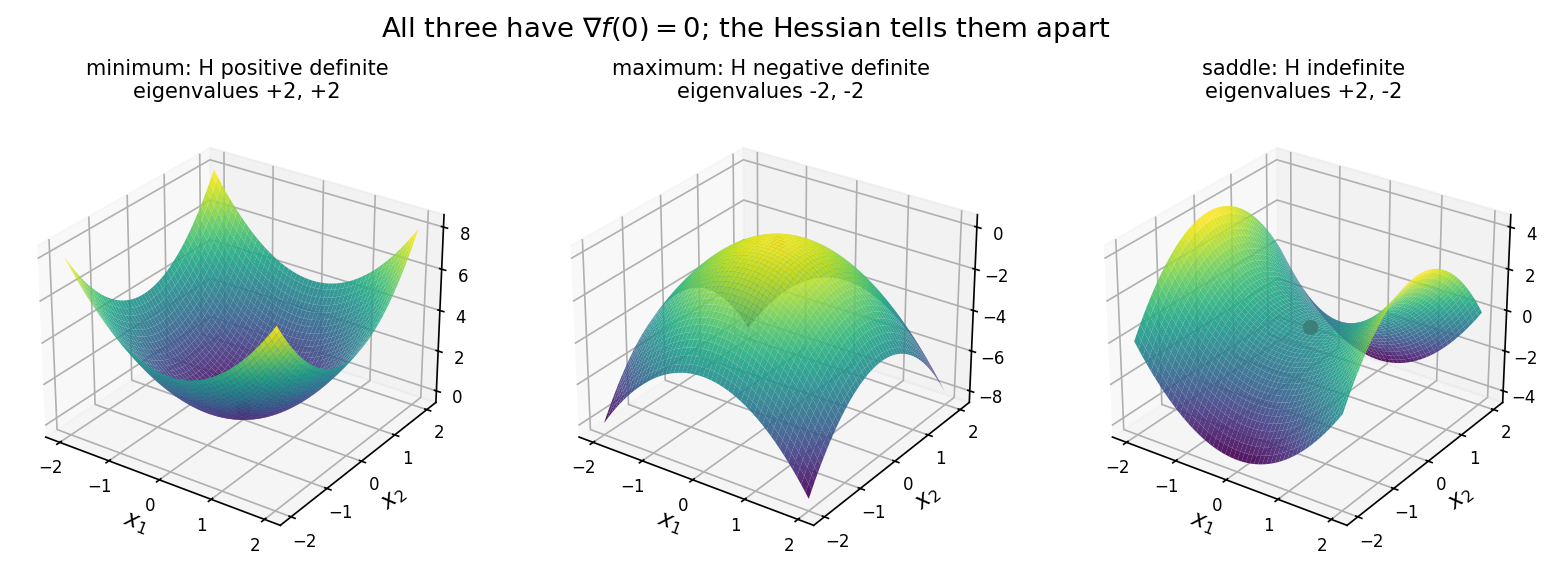
Points where are critical or stationary points. A local minimum is lower than all neighbouring points, a local maximum is higher, and a saddle point is neither: it is a minimum along some directions and a maximum along others. A global minimum has the lowest value anywhere; a function can have several global minima and many local minima that are not global.
For deep networks we rarely find a true global minimum, and we do not need to. We settle for parameters with a low enough loss that generalize well. In high dimensions, saddle points rather than poor local minima are the more common critical points of many random-like functions, and they can slow gradient-based optimizers because the gradient becomes small near them [8]. Figure 1 shows the three kinds of critical point.
Jacobian and Hessian matrices
Plain version. The Jacobian collects all first derivatives of a vector-valued function. The Hessian collects all second derivatives of a scalar function: it tells you how the slope itself changes, which is curvature.
Definitions
For a function , the Jacobian has entries
Row is the gradient of output . Backpropagation is repeated multiplication by Jacobians; reverse-mode automatic differentiation computes vector–Jacobian products without ever forming , which is why a gradient costs only a small constant multiple of one function evaluation [11].
For a scalar function , the Hessian is the Jacobian of the gradient:
Wherever the second partial derivatives are continuous, the order of differentiation does not matter, so : the Hessian is symmetric. A real symmetric matrix has real eigenvalues and an orthonormal basis of eigenvectors . The second derivative in a unit direction is . If is an eigenvector , it equals ; for other directions it is a weighted average of the eigenvalues, with weights between 0 and 1 that sum to 1. So is the largest curvature in any direction and the smallest.
What a gradient step really does: second-order Taylor expansion
Write and . The second-order Taylor approximation around is
Substituting a gradient step gives
The three terms are the current value, the improvement predicted by the slope, and a correction for curvature. If , the approximation keeps decreasing as grows (until the approximation itself stops being valid). If , the curvature term eventually wins, and the approximation is minimized at
In the worst case, is aligned with the eigenvector of and . Large curvature forces small steps.
The second derivative test
At a critical point () the Taylor expansion reduces to the quadratic term, so the Hessian decides what kind of point it is:
- positive definite (all ): local minimum.
- negative definite (all ): local maximum.
- has at least one positive and at least one negative eigenvalue: saddle point.
- Otherwise (some and the rest of one sign) the test is inconclusive.
In one dimension a saddle cannot exist; in dimensions it needs only one eigenvalue of the “wrong” sign, which is why saddles become so common as grows [8].
Condition number of the Hessian: why gradient descent zigzags
On the quadratic with symmetric positive definite, gradient descent is linear: . Expanding in the eigenvectors of , the component along is multiplied by at every step. Therefore:
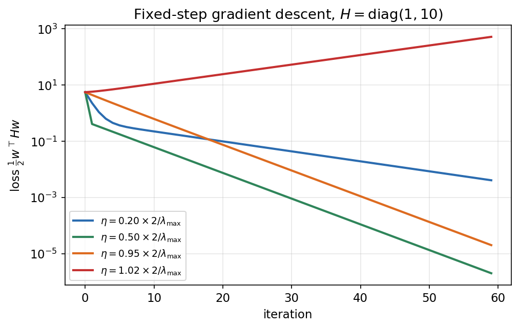
- The iteration is stable only if for every , that is, .
- The slowest direction is the flat one, contracting by per step.
- The best fixed step, , contracts the error by per step, with the condition number of the Hessian.
So a large condition number means one direction wants tiny steps (or it diverges) while another direction needs many steps to make progress. Gradient descent wastes its time bouncing across the steep walls of a narrow valley — the zigzag in Figure 2 — while creeping along the valley floor. Badly scaled input features produce exactly this situation, which is one reason standardization and normalization layers speed up training.
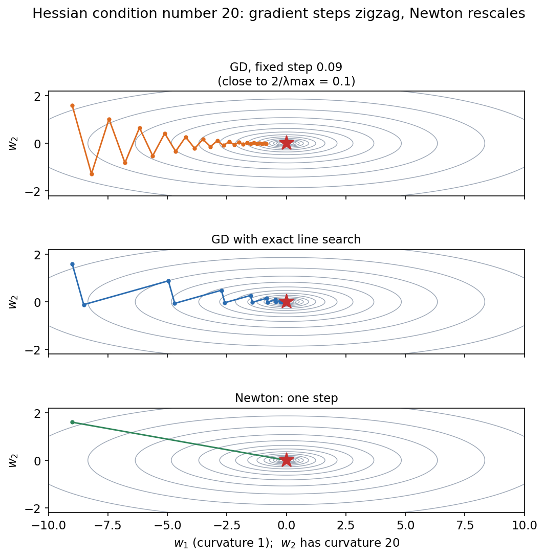
Figure 3 shows the stability limit numerically. Below the loss decreases; just above it the steep component grows by a factor every step and the loss explodes.
Code · Python · 25 lines
import numpy as np

H = np.diag([1.0, 25.0])                     # Hessian: condition number 25
f = lambda w: 0.5 * w @ H @ w
grad = lambda w: H @ w

def run_gd(eta, steps=50):
    w = np.array([10.0, 1.0])
    for _ in range(steps):
        w = w - eta * grad(w)
    return f(w)

lam_max = np.linalg.eigvalsh(H).max()
for eta in (0.01, 0.07, 0.079, 0.081):       # stability limit 2/25 = 0.08
    print(f"eta={eta:<6} loss after 50 steps: {run_gd(eta):.3e}")

# Exact line search along -g for a quadratic: eps* = g'g / g'Hg
w = np.array([10.0, 1.0])
g = grad(w)
eps_star = (g @ g) / (g @ H @ g)
print("optimal step along the gradient:", round(eps_star, 4))

# One Newton step lands on the minimizer of a quadratic
w_newton = w - np.linalg.solve(H, g)
print("after one Newton step:", w_newton)
The output shows the whole story: is stable but slow (loss after 50 steps), reaches , is barely stable and the steep component still oscillates (loss about ), and diverges (loss ). The optimal step along the first gradient is , and one Newton step lands exactly on .
Second-order methods
Plain version. Newton’s method uses curvature to rescale the gradient. Near a well-behaved minimum this can help; indefinite curvature can produce a poor direction.
Newton’s method
Setting the gradient of the second-order Taylor approximation to zero gives the Newton step
On a positive-definite quadratic this jumps to the minimum in one step (Figure 2, bottom). On a general function that is locally close to a positive-definite quadratic, iterating the update converges much faster than gradient descent — quadratically near the solution, under standard assumptions [6]. The cost is the Hessian: storing it takes memory and solving with it time, impossible for a network with parameters.
There is also a more fundamental problem for non-convex objectives. Newton’s method finds a point where the gradient vanishes, and it treats a saddle the same way as a minimum: near a saddle, the Newton step points toward it. In a landscape full of saddles, plain Newton is attracted to exactly the points we want to escape. Dauphin et al. proposed a “saddle-free Newton” method that rescales by the absolute values of the Hessian eigenvalues to avoid this [8]. Gradient descent, by contrast, is not attracted to saddles in the same way, although it can move slowly near them.
Quasi-Newton methods and L-BFGS
Quasi-Newton methods build an approximation (or of its inverse) from gradients alone. After a step with gradient change , they require the secant condition , which says the model’s curvature along the step matches the observed change in slope. BFGS is the most widely used update of this kind; L-BFGS (limited-memory BFGS) stores only the last pairs and applies the inverse-Hessian approximation implicitly in time [6], [10]. L-BFGS is excellent for smooth, deterministic, medium-sized problems (logistic regression, style transfer on one image, fitting a few thousand parameters); its curvature estimates suffer when gradients are noisy mini-batch estimates.
Hessian-vector products
Many curvature-aware methods never need itself, only products . These can be computed exactly at roughly the cost of a couple of gradient evaluations, because is the gradient of a scalar; Pearlmutter showed how to do this with automatic differentiation [9]. A finite-difference version, , is a useful check. Power iteration with Hessian-vector products estimates , which is how researchers track the sharpness of the loss during training.
Code · Python · 21 lines
import numpy as np

rng = np.random.default_rng(0)
X = rng.normal(size=(50, 4))
y = (rng.random(50) < 0.5).astype(float)

def grad(w):                                   # logistic regression, mean loss
    p = 1 / (1 + np.exp(-(X @ w)))
    return X.T @ (p - y) / len(y)

def hessian(w):
    p = 1 / (1 + np.exp(-(X @ w)))
    return (X.T * (p * (1 - p))) @ X / len(y)

w = rng.normal(size=4)
v = rng.normal(size=4)
r = 1e-5
hvp_fd = (grad(w + r*v) - grad(w - r*v)) / (2*r)   # never forms H
print("Hv (finite diff):", hvp_fd.round(6))
print("Hv (explicit)   :", (hessian(w) @ v).round(6))
print("eigenvalues of H:", np.linalg.eigvalsh(hessian(w)).round(4))
Both products agree to six decimals, and all Hessian eigenvalues are positive: logistic regression is convex, so its Hessian is positive semidefinite everywhere.
Lipschitz continuity and convexity
Deep-learning objectives come with few guarantees, but two properties explain much of the theory. A function is Lipschitz continuous with constant if for all : its rate of change is bounded. When the gradient is -Lipschitz (the function is “-smooth”), the curvature is bounded by , and a gradient step with is guaranteed not to increase the function:
This is the general form of the "" rule above, and it is the starting point of most convergence proofs [7], [14].
A function is convex if its Hessian is positive semidefinite everywhere (for twice-differentiable functions). Convex functions have no saddles and no spurious local minima: every local minimum is global. Least squares, logistic regression and support vector machines are convex; deep networks are not. Convex optimization is the source of many tools, such as duality and the KKT conditions below, that deep learning borrows [7].
Constrained optimization
Plain version. Constraints restrict the allowed solutions. Projection returns an update to the feasible region; Lagrange multipliers describe how constraints enter the optimality conditions.
Projected gradient descent
We want to minimize over a feasible set . When projecting onto is easy, take a normal gradient step and then return to the nearest feasible point:
For the Euclidean ball the projection is : rescale if too long. Max-norm constraints on weights, clipping parameters into a box, and projecting onto the probability simplex all follow this pattern. Another option is to reparameterize so the constraint holds automatically, for example for a vector on a circle, or a softmax to produce probabilities.
The generalized Lagrangian
A more general approach describes the feasible set with equality constraints and inequality constraints :
Introduce one KKT multiplier for each constraint, for equalities and for inequalities, and define the generalized Lagrangian
The constrained problem is equivalent to the unconstrained min–max problem
Why does this work? If violates a constraint, the inner maximization can drive to by choosing a large multiplier, so infeasible points are never chosen. If is feasible, the best the inner maximization can do is set the terms to zero (equalities are already 0; for the best non-negative makes ), so the value is exactly [1].
The KKT conditions
At a solution (under mild regularity conditions called constraint qualifications), there exist multipliers satisfying the Karush–Kuhn–Tucker (KKT) conditions [1], [7]:
- Stationarity: .
- Primal feasibility: all constraints hold at .
- Dual feasibility: .
- Complementary slackness: for every .
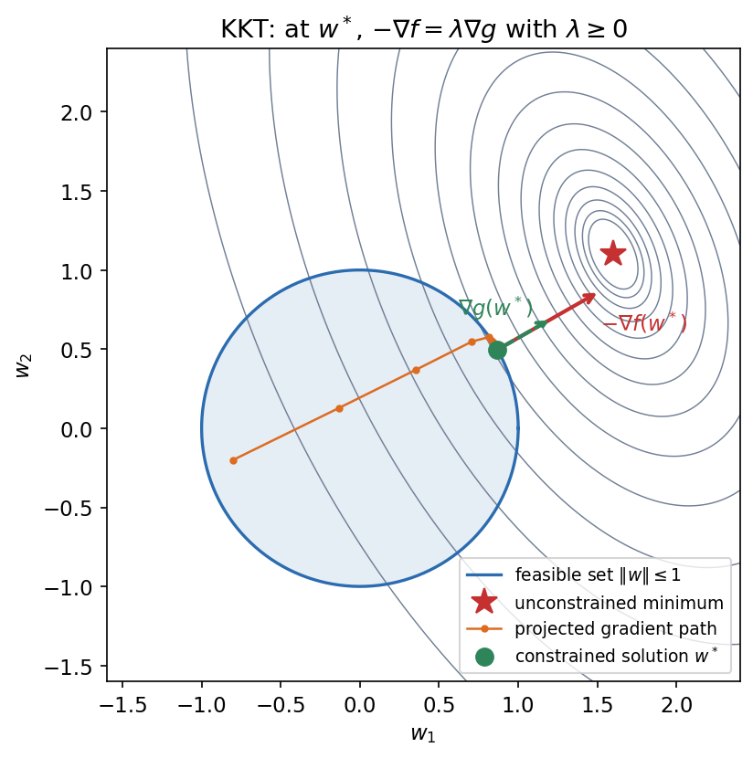
Complementary slackness says each inequality is either active (: the solution sits on the boundary and the constraint pushes back with ) or inactive (: the constraint does not matter locally and ). Geometrically, stationarity says that at an active constraint the downhill direction points straight out of the feasible set, parallel to ; any feasible move would go uphill (Figure 4). For convex problems the KKT conditions are also sufficient for optimality [7].
Worked example: least squares with a norm constraint
Following the example in [1], minimize the squared error , with and , subject to . The Lagrangian is
Stationarity gives , so
This is ridge regression with penalty . If the ordinary least-squares solution already satisfies , the constraint is inactive, , and we are done. Otherwise the constraint is active, and we increase until ; because decreases monotonically in , a bisection finds it. This is also how the inner maximization over behaves: the multiplier grows while the constraint is violated and stops when it is just satisfied. The code solves the problem both ways and checks all four KKT conditions.
Code · Python · 40 lines
import numpy as np

# minimize ||Aw - b||^2  subject to  ||w||^2 <= r^2
rng = np.random.default_rng(1)
A = rng.normal(size=(30, 5))
b = rng.normal(size=30)
r = 0.2

def w_of(lam):                                # stationarity of the Lagrangian
    return np.linalg.solve(A.T @ A + lam * np.eye(5), A.T @ b)

w_ls = w_of(0.0)
print("unconstrained norm:", np.linalg.norm(w_ls).round(3))

lo, hi = 0.0, 1e6                             # find lambda with ||w|| = r
for _ in range(200):
    mid = 0.5 * (lo + hi)
    if np.linalg.norm(w_of(mid)) > r:
        lo = mid
    else:
        hi = mid
lam = hi
w = w_of(lam)
print("lambda:", round(lam, 3), " ||w||:", np.linalg.norm(w).round(6))

# KKT checks
stationarity = 2 * A.T @ (A @ w - b) + 2 * lam * w
print("stationarity residual:", np.abs(stationarity).max())
print("primal feasible:", w @ w <= r**2 + 1e-9, " dual feasible:", lam >= 0)
print("complementary slackness:", lam * (w @ w - r**2))

# Projected gradient descent reaches the same point
L = 2 * np.linalg.eigvalsh(A.T @ A).max()     # Lipschitz constant of the gradient
v = np.zeros(5)
for _ in range(5000):
    v = v - (1 / L) * 2 * A.T @ (A @ v - b)
    n = np.linalg.norm(v)
    if n > r:
        v = v * (r / n)                       # projection onto the ball
print("projected GD matches KKT solution:", np.allclose(v, w, atol=1e-6))
The unconstrained solution has norm , larger than , so the constraint is active. Bisection finds , the stationarity residual is about , complementary slackness holds, and projected gradient descent with step converges to the same vector. Note how , the Lipschitz constant of the gradient, sets a safe step size, exactly as in the previous section.
Checking derivatives
Plain version. Check that the gradient your code computes matches how the loss actually changes when you nudge the parameters.
A central finite difference estimates a partial derivative,
where is the -th standard basis vector and a small step. Its truncation error (from ignoring higher-order Taylor terms) is , better than the of the forward difference . But the numerator subtracts two nearly equal numbers, so its roundoff error grows like . The total error is smallest at an intermediate step — roughly for central differences and for forward differences, when and its derivatives have unit scale. Figure 5 shows the resulting V-shaped curves, and why float32 gradient checks are much less precise than float64 ones.
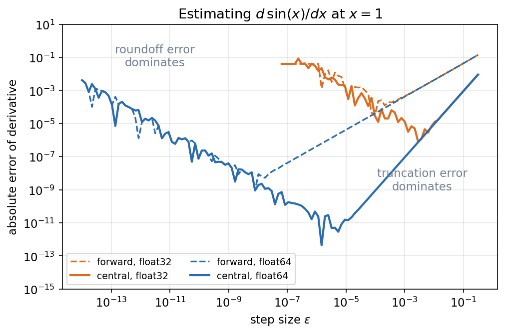
Practical rules: use float64 for checks; try several step sizes; compare with a relative error such as ; and test at smooth points. ReLU exactly at zero is not differentiable, so there is no single derivative to match there. For many parameters, a directional check is cheaper: choose a random unit vector and compare with a finite difference along — one pair of function evaluations instead of .
Code · Python · 16 lines
import numpy as np

rng = np.random.default_rng(0)
X = rng.normal(size=(20, 5))
y = rng.normal(size=20)
w = rng.normal(size=5)
v = rng.normal(size=5)
v /= np.linalg.norm(v)
def loss(w):
    return .5*np.mean((X@w-y)**2)
grad = X.T@(X@w-y)/len(y)
eps = 1e-5
numeric = (loss(w+eps*v)-loss(w-eps*v))/(2*eps)
analytic = grad@v
assert np.allclose(numeric, analytic, rtol=1e-6, atol=1e-8)
print("directional derivative:", numeric, analytic)
The two numbers agree to about nine significant digits. A passing check confirms a derivative, not the intended task. A wrong reduction, accidental broadcasting or target leakage can define a differentiable but incorrect objective whose gradient passes [11]. An accidental detach is different: if the forward value still changes with an input but autograd cuts that dependency, finite differences can expose the mismatch [24]. Test the relevant inputs at smooth points, hold randomness fixed, and also check loss values on cases with known answers.
Mixed precision
Plain version. Doing most arithmetic in 16-bit numbers halves memory traffic and uses fast hardware units, but 16 bits are not enough for everything. Keep a few sensitive quantities in 32 bits.
Mixed-precision training, as introduced by Micikevicius et al. [12], combines three ideas:
- Keep a float32 master copy of the weights. An update smaller than about times the weight it is added to rounds away entirely in float16 (the same effect as above), and many updates are that small.
- Use loss scaling for float16: multiply the loss by a factor before backpropagation so small gradients do not underflow below float16’s smallest subnormal (), then divide the gradients by before the update. Dynamic loss scaling reduces when an overflow (inf or NaN) appears and skips that step.
- Accumulate dot products and reductions in float32 even when inputs are float16.
bfloat16 has the same 8-bit exponent as float32, so it rarely needs loss scaling; Kalamkar et al. found bfloat16 training reached float32 results across a range of models without changing hyperparameters [5]. The price is precision: with , bfloat16 cannot represent distinctly from 1, so long sums and weight updates still need float32 accumulation.
Loss scaling protects small float16 gradients; it cannot repair an invalid objective or an overflow elsewhere in the network (an attention logit or a normalization statistic, for example). Changing precision can also change optimization trajectories and outputs, especially for reductions and long training runs. Validate on the target hardware; a smaller dtype does not guarantee that every operation becomes faster [13].
Optional: Mixed Precision Training (in the Paper guides). Read the original figure, evidence, design choices and limitations.
A debugging order for non-finite values
When a loss becomes nan or inf, resist the urge to clip everything. Find the first operation that produced a non-finite value, then ask which of this chapter’s failure modes it is. A useful order:
- Inputs: check shapes, ranges, dtypes and missing values. A single NaN pixel or an un-normalized 0–255 image changes everything downstream.
- Forward pass: check that activations and the loss are finite. Look for
exp,log, division,sqrtand normalization layers with near-zero variance. - Loss: use logits-based losses (
cross_entropy,binary_cross_entropy_with_logits) rather than probabilities followed bylog. - Gradients: run a gradient check on a tiny model; inspect per-layer gradient norms.
- Updates: compare the update size with the weight size; a learning rate above the curvature limit causes oscillation and divergence even with perfect arithmetic.
- Precision: reproduce in float32 (or float64) before adding mixed precision or compilation.
Overfit a tiny batch first to establish that the pipeline can learn. Gradient-norm clipping bounds the gradient passed to the optimizer; it does not directly bound an adaptive optimizer’s update, and it does not make NaN gradients meaningful. ML 02 develops optimizers and normalization in more detail.
Modern view
The core ideas of this chapter are decades old, but they are at the centre of current research because models are larger, training runs are longer, and hardware keeps pushing precision downward.
Optimization theory for large-scale learning. Bottou, Curtis and Nocedal’s SIAM Review survey [14] is the standard map of the field. It explains why stochastic gradient methods dominate large-scale machine learning (cheap noisy steps beat expensive exact ones when data are redundant), analyses their convergence under smoothness assumptions like the Lipschitz condition above, and organizes improvements into two families: noise reduction (larger or growing batches, variance reduction, iterate averaging) and second-order methods (Hessian-free Newton, Gauss–Newton, quasi-Newton, natural gradient and diagonal scaling). Nocedal and Wright [6] and Boyd and Vandenberghe [7] remain the reference textbooks for the deterministic and convex theory, and Baydin et al. [11] survey the automatic differentiation that makes gradients cheap.
What the loss surface actually looks like. Dauphin et al. [8] argued that saddle points, not poor local minima, are the main obstacle in high-dimensional non-convex optimization. Later, Cohen et al. [15] observed that full-batch gradient descent on neural networks typically operates at the “edge of stability”: the largest Hessian eigenvalue rises until it hovers just above — precisely the classical stability limit derived above — while the loss keeps decreasing over long time scales, though not monotonically. The classical quadratic analysis predicts divergence there, so explaining this regime remains an open theoretical problem.
Curvature-aware optimizers. Full Newton is impossible at scale, but structured approximations are practical. K-FAC [16] approximates the Fisher information matrix (a positive-semidefinite curvature matrix closely related to the Gauss–Newton approximation of the Hessian) with Kronecker products of small per-layer matrices, so inverting it is cheap. Shampoo [17] keeps one preconditioning matrix per tensor dimension. More recently, Muon applies an approximate orthogonalization to each weight matrix’s update; Liu et al. [18] report that, with suitable weight decay and per-parameter update scaling, it trains large language models with roughly twice the computational efficiency of their adaptive-optimizer baseline in their experiments. These methods all revisit the question this chapter asks with the Hessian: how should a step be rescaled direction by direction?
Lower precision. The format story continues from float16 with loss scaling [12] and bfloat16 [5] to 8-bit floating point. Micikevicius et al. [19] proposed two FP8 encodings, E4M3 (more precision) and E5M2 (more range), and showed training results comparable to 16-bit baselines across image and language models. The range–precision trade-off in the table above is exactly what these designs balance, and the IEEE 754 rules [3] are what they relax. Per-tensor or per-block scaling factors play the role that loss scaling played for float16.
Stable softmax at scale. The max-subtraction trick has a streaming version. Milakov and Gimelshein [20] showed that a softmax normalizer can be computed in one pass by keeping a running maximum and rescaling the running sum whenever the maximum changes. FlashAttention [21] builds on this idea: it computes exact attention block by block in fast on-chip memory, never materializing the full attention matrix, and FlashAttention-3 [22] extends it to FP8 with block quantization and “incoherent processing” to reduce quantization error. The core of the online trick fits in a few lines:
Code · Python · 17 lines
import numpy as np

def online_logsumexp(chunks):
    m, s = -np.inf, 0.0                 # running max and rescaled running sum
    for c in chunks:
        m_new = max(m, c.max())
        s = s * np.exp(m - m_new) + np.exp(c - m_new).sum()
        m = m_new
    return m + np.log(s)

rng = np.random.default_rng(0)
z = rng.normal(0, 50, size=10_000)
chunks = np.array_split(z, 37)          # seen one block at a time
m = z.max()
reference = m + np.log(np.exp(z - m).sum())
print(online_logsumexp(chunks), reference)
assert np.isclose(online_logsumexp(chunks), reference)
Both values print as , identical to the last digit shown, although the online version never sees all logits at once. ML 05 covers attention itself, and ML 11 covers quantization for deployment.
Open problems. Why gradient methods succeed at the edge of stability; how to make low-precision (8-bit and below) training as robust as float32 without hand-tuned scaling; how to make curvature-aware optimizers cheap and robust enough to replace first-order defaults; and how to obtain reproducible results when parallel reductions change summation order.
Key takeaways
- Exponent bits set range and fraction bits set precision; subnormal numbers have different relative-precision behavior.
- Use stable formulas such as log-sum-exp and logits-based losses before increasing precision.
- Conditioning measures input sensitivity; a stable algorithm cannot eliminate an ill-conditioned problem’s sensitivity.
- Curvature controls safe step sizes for quadratic objectives; general nonconvex losses require additional care.
- Projection enforces feasibility; KKT conditions require regularity assumptions and are not a universal certificate of global optimality.
- Check gradients at smooth points with suitable precision and step sizes; validate mixed precision on the actual computation.
Exercises
- Softmax shift. Prove that softmax is invariant under , and show that with the denominator lies in .
Hint
The shared factor cancels between numerator and denominator. After the shift, every term is in and the largest equals 1, so the sum of terms is between 1 and . It can therefore neither overflow nor underflow to 0.
- Finite-difference sweep. For at , compute forward and central differences for in float32 and float64. At which is each error smallest? Compare with and .
Hint
For float64, , so (forward) and (central). For float32, , giving about and . The observed minima should be within an order of magnitude of these, and the error at the minimum is roughly and respectively.
- Stability limit. For with , find the largest stable fixed learning rate and the step size that minimizes the worst-case contraction factor. How many iterations does that best step need to reduce the error by a factor of ?
Hint
Stability requires . The best step is , with contraction . Solve : iterations. A Newton step would need one.
- Classify critical points. Find and classify the critical points of .
Hint
gives and . The Hessian is : at it is , positive definite, a local minimum; at it is , indefinite, a saddle. Neither is a global minimum because as . Starting Newton’s method near converges to the saddle.
- KKT on the simplex. Minimize subject to and , for . Write the Lagrangian and the KKT conditions, and find the solution.
Hint
with . Stationarity gives ; complementary slackness gives . Guess that only the first two are positive: , so and . Check: , so with . This is the Euclidean projection onto the probability simplex.
- A correct gradient of the wrong loss. Change a mean reduction into a sum in the gradient-check example. Does the check still pass? Is autograd wrong? What else changes in training?
Hint
If you change both the loss and the analytic gradient consistently, the check passes: the derivative is correct for the new objective. Nothing is wrong with autograd. But the gradient is now times larger, so the largest stable learning rate shrinks by , and in a multi-term loss the balance between terms changes. A gradient check cannot tell you that you chose the wrong objective.
References
- I. Goodfellow, Y. Bengio and A. Courville, Deep Learning, MIT Press, 2016, ch. 4 (Numerical Computation) and ch. 8. Book
- D. Goldberg, “What Every Computer Scientist Should Know About Floating-Point Arithmetic,” ACM Computing Surveys, vol. 23, no. 1, pp. 5–48, 1991. DOI
- IEEE, “IEEE Standard for Floating-Point Arithmetic,” IEEE Std 754-2019, 2019. DOI
- N. J. Higham, Accuracy and Stability of Numerical Algorithms, 2nd ed., SIAM, 2002. DOI
- D. Kalamkar et al., “A Study of BFLOAT16 for Deep Learning Training,” arXiv:1905.12322, 2019. arXiv
- J. Nocedal and S. J. Wright, Numerical Optimization, 2nd ed., Springer, 2006. DOI
- S. Boyd and L. Vandenberghe, Convex Optimization, Cambridge University Press, 2004. Book
- Y. N. Dauphin, R. Pascanu, C. Gulcehre, K. Cho, S. Ganguli and Y. Bengio, “Identifying and Attacking the Saddle Point Problem in High-Dimensional Non-Convex Optimization,” NeurIPS, 2014. Paper
- B. A. Pearlmutter, “Fast Exact Multiplication by the Hessian,” Neural Computation, vol. 6, no. 1, pp. 147–160, 1994. DOI
- D. C. Liu and J. Nocedal, “On the Limited Memory BFGS Method for Large Scale Optimization,” Mathematical Programming, vol. 45, pp. 503–528, 1989. DOI
- A. G. Baydin, B. A. Pearlmutter, A. A. Radul and J. M. Siskind, “Automatic Differentiation in Machine Learning: a Survey,” Journal of Machine Learning Research, vol. 18, no. 153, pp. 1–43, 2018. arXiv
- P. Micikevicius et al., “Mixed Precision Training,” ICLR, 2018. arXiv
- PyTorch documentation, “Numerical Accuracy.” Documentation
- L. Bottou, F. E. Curtis and J. Nocedal, “Optimization Methods for Large-Scale Machine Learning,” SIAM Review, vol. 60, no. 2, pp. 223–311, 2018. DOI
- J. M. Cohen, S. Kaur, Y. Li, J. Z. Kolter and A. Talwalkar, “Gradient Descent on Neural Networks Typically Occurs at the Edge of Stability,” ICLR, 2021. arXiv
- J. Martens and R. Grosse, “Optimizing Neural Networks with Kronecker-factored Approximate Curvature,” ICML, 2015. Paper
- V. Gupta, T. Koren and Y. Singer, “Shampoo: Preconditioned Stochastic Tensor Optimization,” ICML, 2018. Paper
- J. Liu, J. Su, X. Yao et al., “Muon is Scalable for LLM Training,” arXiv:2502.16982, 2025. arXiv
- P. Micikevicius et al., “FP8 Formats for Deep Learning,” arXiv:2209.05433, 2022. arXiv
- M. Milakov and N. Gimelshein, “Online Normalizer Calculation for Softmax,” arXiv:1805.02867, 2018. arXiv
- T. Dao, D. Y. Fu, S. Ermon, A. Rudra and C. Ré, “FlashAttention: Fast and Memory-Efficient Exact Attention with IO-Awareness,” NeurIPS, 2022. Paper
- J. Shah, G. Bikshandi, Y. Zhang, V. Thakkar, P. Ramani and T. Dao, “FlashAttention-3: Fast and Accurate Attention with Asynchrony and Low-precision,” NeurIPS, 2024. Paper
- NumPy developers, “numpy.linalg.cond,” NumPy documentation, accessed 2026-11-05. Documentation
- PyTorch contributors, “torch.autograd.gradcheck.gradcheck,” PyTorch documentation, accessed 2026-11-05. Documentation
Check your understanding
This tutorial has 6 exercises. Can you solve them without opening the hints?
Go to the exercises ↑Next ML 02 · Neural Networks from Perceptron to Deep Networks · 37 min