ML 06A · Linear Factor Models and Autoencoders
Needs: ML 01B · Probability and Information Theory, ML 02 · Neural Networks from Perceptron to Deep Networks
Navigate: this page and this track: Navigate: this page and this track
On this page
- What you’ll learn1 min
- The big picture2 min
- PCA: the best linear reconstruction subspace3 min
- Probabilistic PCA and factor analysis2 min
- Independent component analysis (ICA)2 min
- Sparse coding2 min
- Nonnegative matrix factorization (NMF)2 min
- Linear autoencoders and PCA1 min
- Nonlinear autoencoders1 min
- Regularized autoencoders: sparse, denoising and contractive3 min
- The manifold view2 min
- From autoencoders to VAEs2 min
- Modern view3 min
- Key takeaways1 min
- Exercises2 min
- Paper guides
- References
Machine Learning
Explore this chapter 2 interactive experiments
Transform a real photo with an 8 × 8 block DCT or a Haar wavelet, round every coefficient to a coarse step, and see where the lost information shows up.
What you’ll learn
- Explain how latent factors describe correlated measurements.
- Compare PCA, probabilistic PCA and factor-analysis noise assumptions.
- Distinguish independence, sparsity and nonnegativity constraints.
- Relate linear and nonlinear autoencoders to reconstruction objectives.
- Understand manifold assumptions and why reconstruction alone does not define sampling.
The big picture
An 8 × 8 digit image has 64 pixel values, and a phone photo has millions. Yet the meaningful variation in a collection of such images depends on far fewer underlying quantities: which digit it is, the stroke thickness, the slant, the position, the lighting. A factor model tries to explain each observation through a handful of hidden (latent) coordinates. An autoencoder is a neural network that learns to squeeze an input into such coordinates and expand it back again.
Why spend a whole chapter on this? Because almost every idea in modern representation learning and generative modeling has an ancestor here. Dimensionality reduction for visualization, denoising, compression, anomaly detection, the “tokenizers” that turn images into compact codes for diffusion models, and the probabilistic machinery of VAEs all start from the same question: what small set of causes could have produced these observations? The progression from linear factor models to autoencoders follows Goodfellow, Bengio and Courville [1, ch. 13–14] and Murphy [2]; Bengio, Courville and Vincent’s review [3] gives the broader motivation for why learned representations matter.
One template, many models
Every method in this chapter fits the same template. There is an encoder that maps an observation to a code , and a decoder that maps a code back to a reconstruction . The models differ in three choices:
| Choice | Options in this chapter |
|---|---|
| Shape of encoder/decoder | linear (PCA, factor analysis, ICA, NMF, sparse coding) or nonlinear (deep autoencoders) |
| Size of the code | undercomplete (: the bottleneck forces compression) or overcomplete (: something else must stop the model from copying) |
| Extra assumption or penalty | Gaussian noise (PPCA, FA), independence and non-Gaussianity (ICA), sparsity (sparse coding, sparse autoencoders), nonnegativity (NMF), robustness to corruption (denoising), insensitivity to small input changes (contractive) |
Keep this table in mind. When two methods disagree, it is almost always because they made a different choice in one of these rows, not because one of them is “wrong.”
PCA: the best linear reconstruction subspace
Plain version. Find a few orthogonal directions such that, if you keep only the coordinates of each example along those directions, you lose as little as possible.
Let hold centered examples as rows (the column means have been subtracted). PCA chooses a matrix with orthonormal columns that minimizes the squared reconstruction error
Here is the Frobenius norm (the square root of the sum of squared entries), are the codes (also called scores), and is the reconstruction. The encoder is and the decoder is : PCA is already an autoencoder, just a linear one with tied weights.
Where the solution comes from
Two equivalent views lead to the same answer.
Maximum variance. Take a single unit vector . The variance of the projected data is , where is the sample covariance. Maximize subject to with a Lagrange multiplier :
So must be an eigenvector of , and the variance it captures is its eigenvalue . The best direction is the eigenvector with the largest eigenvalue; the next best direction, constrained to be orthogonal to the first, is the second eigenvector, and so on.
Minimum reconstruction error. Because has orthonormal columns, the error splits into “total variance minus kept variance.” Minimizing the error is therefore the same as maximizing the kept variance, and the residual equals the sum of the discarded eigenvalues (times ). The Eckart–Young theorem states the same result in matrix language: truncating the singular value decomposition to its largest singular values gives the best rank- approximation of in Frobenius norm. The PCA directions are the first right singular vectors (columns of ), and the covariance eigenvalues are .
Code: PCA from the SVD
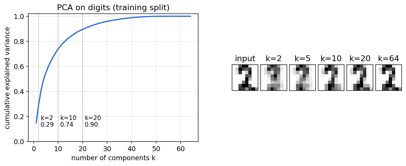
The snippet fits PCA on the training split of scikit-learn’s bundled digits, evaluates reconstruction on held-out images, and checks the result against scikit-learn’s own implementation.
Code · Python · 20 lines
import numpy as np
from sklearn.datasets import load_digits
from sklearn.decomposition import PCA
from sklearn.model_selection import train_test_split

X = load_digits().data / 16.
train, test = train_test_split(X, test_size=.2, random_state=0)

mean = train.mean(axis=0)
U, s, Vt = np.linalg.svd(train - mean, full_matrices=False)
var = s**2 / (len(train) - 1)              # eigenvalues of the covariance
ratio = np.cumsum(var) / var.sum()
for k in (2, 10, 20):
    W = Vt[:k].T                            # d x k, orthonormal columns
    rec = (test - mean) @ W @ W.T + mean
    print(f"k={k:2d}  explained={ratio[k-1]:.3f}  "
          f"test MSE={np.mean((test - rec)**2):.4f}")

sk = PCA(n_components=10).fit(train)
print("matches sklearn:", np.allclose(np.abs(sk.components_), np.abs(Vt[:10])))
Output:
Code · 4 lines
k= 2  explained=0.291  test MSE=0.0546
k=10  explained=0.740  test MSE=0.0202
k=20  explained=0.896  test MSE=0.0084
matches sklearn: True
The np.abs in the last line is not a hack: each principal direction is only defined up to sign, because and span the same line. Note that the mean is estimated on the training split only and reused for the test split; estimating it on test data would leak information.
What PCA does not promise
Three cautions follow directly from the objective.
- Centering and scaling change the answer. Without centering, the first “component” mostly points at the mean. Standardizing every feature to unit variance gives each pixel equal weight, so raw-pixel PCA and standardized PCA solve different problems.
- Variance is not relevance. The direction of largest variance can be lighting or background rather than the class you care about. PCA is unsupervised; it maximizes retained variance, not class separation (that is the job of methods such as linear discriminant analysis).
- PCA is linear. If the data lie on a curved surface, a flat subspace may need many dimensions to describe what is really a low-dimensional shape. We return to this in the manifold section.
Probabilistic PCA and factor analysis
Plain version. Instead of just finding a subspace, write down a story for how the data were generated: draw a few hidden factors, mix them linearly, then add noise. Then fit that story by maximum likelihood.
Both models share the generative equation
where is the mean, is the loading matrix (how each factor shows up in each measured coordinate), is the vector of latent factors, and is noise independent of . They differ only in the noise.
Probabilistic PCA (PPCA)
In PPCA [4], the noise is isotropic, : every coordinate gets the same noise variance. Integrating out gives a Gaussian marginal
The covariance has a clear interpretation: a low-rank part that the factors explain, plus a constant “floor” that they do not. Tipping and Bishop showed that the maximum-likelihood solution is available in closed form [4]:
where holds the top eigenvectors of the sample covariance, their eigenvalues , and is any orthogonal matrix. In words: the loadings span exactly the PCA subspace, and the noise variance is the average of the variance PCA throws away. PPCA therefore is PCA, plus a likelihood. That likelihood is useful: you can compare models with different on held-out data, handle missing values with expectation–maximization (EM), and build mixtures of PPCA models.
Given an observation, the posterior over its factors is Gaussian with mean
This is the probabilistic encoder. As it approaches the ordinary PCA projection; for it shrinks codes toward zero, because part of what we see is attributed to noise.
Factor analysis (FA)
Factor analysis keeps the same structure but allows a diagonal noise covariance, with . Each observed coordinate has its own residual noise level , while the latent factors explain the shared covariance between coordinates. The marginal is , and the posterior mean of the factors is .
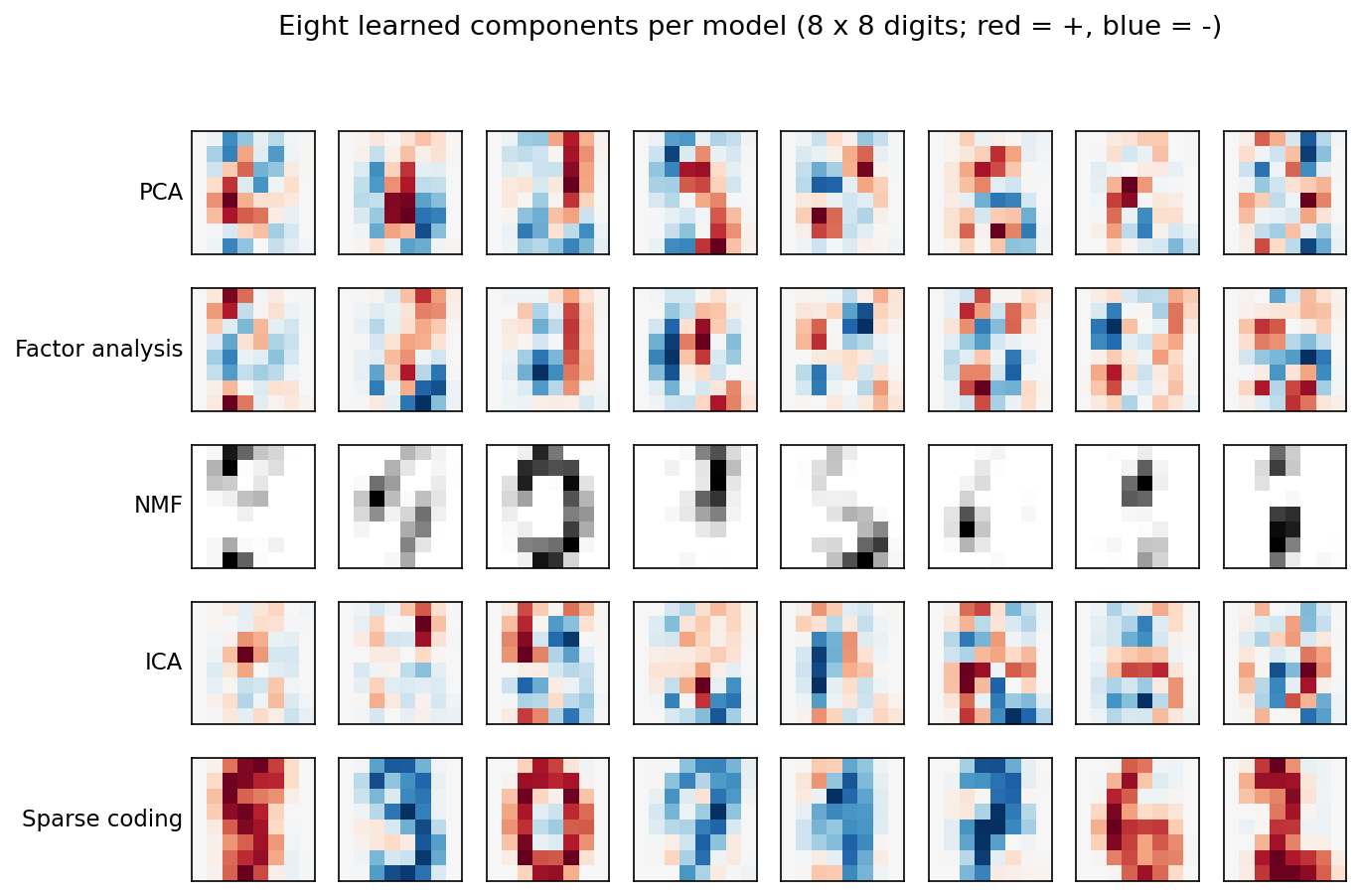
There is no closed-form solution, so FA is fitted with EM or direct likelihood optimization. The extra flexibility matters when measurements come from sensors with unequal noise, or when some pixels are almost constant (such as the always-blank border pixels of the digits). PCA happily spends components on any high-variance coordinate; FA can instead explain an individually noisy coordinate as “noise,” and reserve its factors for correlations.
The rotation problem
Both models share an ambiguity. For any orthogonal , replacing by and by leaves , and hence the distribution of , unchanged, because is still standard normal. The subspace is identified; the individual axes are not. That is why the factor-analysis literature uses rotations such as varimax to pick more interpretable axes, and why a factor is not automatically a physical cause. To pin down individual factors we must assume something beyond Gaussianity, which is precisely what ICA does.
Optional: Probabilistic PCA (in the Paper guides). Read the original figure, evidence, design choices and limitations.
Independent component analysis (ICA)
Plain version. Several people talk at once in a room, and several microphones record different mixtures of their voices. ICA tries to recover each voice by finding mixtures that are as statistically independent, and as non-Gaussian, as possible.
The noise-free ICA model is
where is the observed mixture, is an unknown mixing matrix, and the sources are independent and non-Gaussian. The goal is an unmixing matrix (or a pseudo-inverse) so that recovers the sources [5].
Why non-Gaussianity is the key
The rotation problem from the previous section explains why ICA needs non-Gaussian sources. First whiten the data: transform so that its covariance is the identity (PCA followed by rescaling each component to unit variance does this). After whitening, the remaining unknown is just a rotation. If the sources were Gaussian, every rotation of independent unit Gaussians would again be independent unit Gaussians, so no rotation could be preferred. ICA’s identifiability theorem states the converse: if at most one source is Gaussian, the sources can be recovered up to three harmless ambiguities [5]:
- order (we cannot know which source is “first”),
- sign, and
- scale (a louder source with a quieter mixing column looks the same).
The central limit theorem gives the intuition for how to find the right rotation: a sum of independent variables tends to be more Gaussian than its parts. So the projections of that are least Gaussian are the ones most likely to be single sources rather than mixtures. ICA algorithms therefore maximize a measure of non-Gaussianity. A principled one is negentropy,
where is differential entropy and is a Gaussian with the same variance as . Among all distributions with a given variance, the Gaussian has the largest entropy, so exactly for Gaussian . Because entropy is hard to estimate, the FastICA algorithm approximates negentropy with contrast functions such as , and finds each unmixing direction with a fast fixed-point iteration [5]. Maximizing non-Gaussianity is closely related to minimizing the mutual information between the estimated components and to maximum-likelihood estimation of the ICA model.
Code: unmix three signals
The toy problem uses a sine wave, a square wave and a sawtooth, all non-Gaussian, mixed by a fixed matrix.
Code · Python · 21 lines
import numpy as np
from sklearn.decomposition import FastICA, PCA

rng = np.random.default_rng(0)
t = np.linspace(0, 8, 2000)
S = np.c_[np.sin(2*t),                 # smooth sine
          np.sign(np.sin(3*t)),        # square wave
          2*(t % 1) - 1]               # sawtooth
S += 0.05 * rng.normal(size=S.shape)
A = np.array([[1.0, 1.0, 1.0],
              [0.5, 2.0, 1.0],
              [1.5, 1.0, 2.0]])        # unknown mixing matrix
X = S @ A.T                            # three "microphones"

def best_match(est):
    C = np.abs(np.corrcoef(S.T, est.T)[:3, 3:])
    return np.round(C.max(axis=1), 3)

ica = FastICA(n_components=3, whiten="unit-variance", random_state=0)
print("ICA |corr| with each source:", best_match(ica.fit_transform(X)))
print("PCA |corr| with each source:", best_match(PCA(3).fit_transform(X)))
Output:
Code · 2 lines
ICA |corr| with each source: [0.997 0.999 0.997]
PCA |corr| with each source: [0.689 0.811 0.735]
We compare with absolute correlation and take the best match because ICA returns the sources in arbitrary order, sign and scale. PCA only decorrelates; it finds orthogonal directions of high variance, which here are still mixtures.
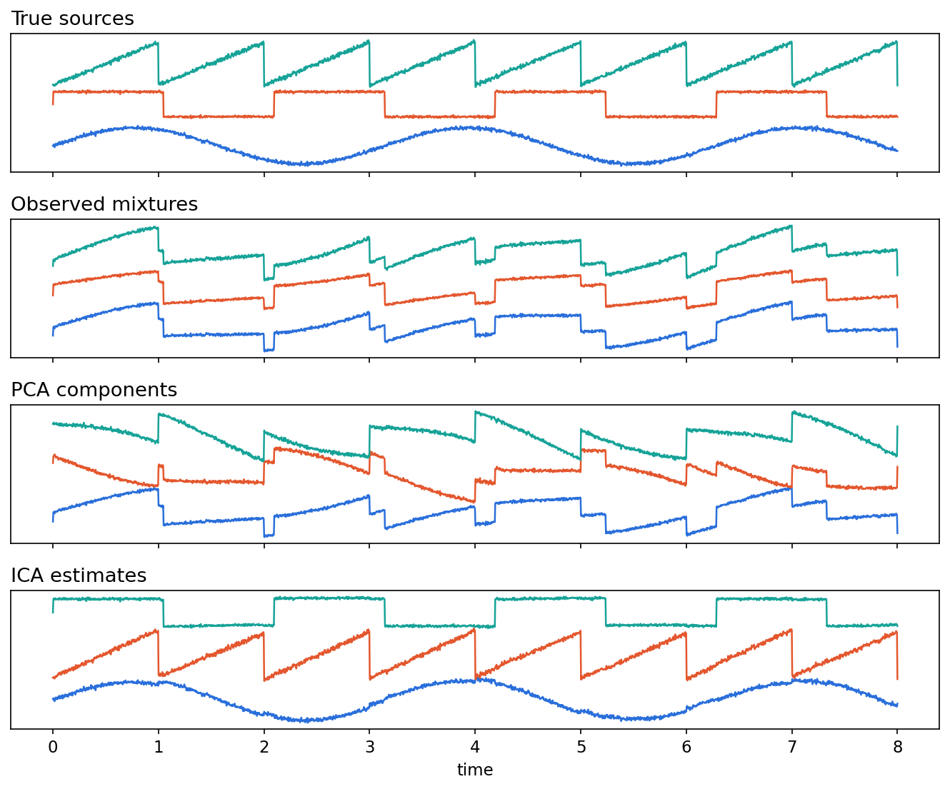
ICA is widely used for separating artifacts in EEG and other sensor recordings. Its assumptions also mark its limits: it needs genuinely independent, non-Gaussian sources and a mixing process that is close to linear and instantaneous. On image patches, ICA tends to learn localized, oriented edge-like filters, which brings us to a closely related idea.
Sparse coding
Plain version. Keep a large dictionary of small patterns (“atoms”) and describe each input using only a few of them at a time.
Sparse coding learns a dictionary and, for each example , a sparse code by solving
The first term asks for accurate reconstruction; the norm pushes most code entries to exactly zero; sets the trade-off. The norm constraint on atoms stops the model from cheating by making atoms huge and codes tiny. The dictionary is often overcomplete (): there are more atoms than pixel dimensions, but only a few are active for any one input.
Olshausen and Field [6] trained this kind of model on patches of natural images and found that the learned atoms were localized, oriented and band-pass, much like the receptive fields of simple cells in the primary visual cortex. The result was influential because it suggested that sparsity alone, without any labels, can explain a known property of biological vision.
Two practical points distinguish sparse coding from the autoencoders later in this chapter:
- Inference is an optimization. Given , finding for a new input means solving a lasso problem. There is no fixed encoder network; the “encoder” is an algorithm. Training alternates between updating the codes (with fixed) and updating the dictionary (with codes fixed).
- Sparsity is a prior. The penalty corresponds to a Laplace prior on the codes, so sparse coding can be read as maximum a posteriori inference in a linear factor model with a sparse, non-Gaussian prior, which is the same family that ICA belongs to.
Code: sparsity versus fidelity
Code · Python · 17 lines
import numpy as np
from sklearn.datasets import load_digits
from sklearn.decomposition import DictionaryLearning
from sklearn.model_selection import train_test_split

X = load_digits().data / 16.
train, test = train_test_split(X, test_size=.2, random_state=0)
for alpha in (0.1, 1.0):
    dl = DictionaryLearning(n_components=32, alpha=alpha, max_iter=30,
                            transform_algorithm="lasso_lars",
                            transform_alpha=alpha, random_state=0)
    dl.fit(train[:600])
    codes = dl.transform(test)
    rec = codes @ dl.components_
    active = np.mean(np.abs(codes) > 1e-8, axis=1).mean()
    print(f"alpha={alpha}: active atoms per image={active*32:.1f}/32, "
          f"test MSE={np.mean((test - rec)**2):.4f}")
Output (about half a minute on a laptop CPU):
Code · 2 lines
alpha=0.1: active atoms per image=17.9/32, test MSE=0.0075
alpha=1.0: active atoms per image=3.0/32, test MSE=0.0401
Raising (here alpha) buys a much sparser description, about three active atoms per image instead of eighteen, at the price of higher reconstruction error. Neither setting is “correct”: a compression codec, a denoiser and an interpretability tool would each choose differently. Note that this dictionary does not subtract a mean, so its error is not directly comparable to the PCA numbers above.
Nonnegative matrix factorization (NMF)
Plain version. Describe each example as an additive mixture of nonnegative parts: you may add strokes, but you may never subtract one.
For data (pixel intensities, word counts, spectra), NMF finds and that minimize a reconstruction criterion such as
where the rows of are nonnegative parts and the rows of are nonnegative mixing weights. Because nothing can cancel, the parts tend to look like pieces of the object rather than the positive-and-negative “ghost” patterns of PCA. Lee and Seung [7] demonstrated this parts-based behavior on faces and text and popularized simple multiplicative update rules for fitting it.
Two cautions. First, parts-based results are a tendency, not a guarantee: on some datasets the factors are not clean parts. Second, the objective is nonconvex in and jointly, so initialization matters and different runs can give different factors. Scikit-learn’s init="nndsvda" uses an SVD-based start to make results more stable.
Code: compare factor reconstructions
This CPU example fits each model on training digits only and evaluates reconstruction on held-out images. It compares different model assumptions; it is not a claim that one method wins every task.
Code · Python · 22 lines
import numpy as np
from sklearn.datasets import load_digits
from sklearn.model_selection import train_test_split
from sklearn.decomposition import PCA, FactorAnalysis, NMF

X = load_digits().data / 16.
train, test = train_test_split(X, test_size=.2, random_state=0)
models = {
    "PCA": PCA(n_components=12),
    "factor analysis": FactorAnalysis(n_components=12, random_state=0),
    "NMF": NMF(n_components=12, init="nndsvda", max_iter=1000,
               random_state=0),
}
for name, model in models.items():
    model.fit(train)
    z = model.transform(test)
    if name == "factor analysis":
        reconstructed = z @ model.components_ + model.mean_
    else:
        reconstructed = model.inverse_transform(z)
    mse = np.mean((test-reconstructed)**2)
    print(name, "held-out reconstruction MSE:", round(mse, 5))
Output:
Code · 3 lines
PCA held-out reconstruction MSE: 0.01652
factor analysis held-out reconstruction MSE: 0.02501
NMF held-out reconstruction MSE: 0.02207
PCA has the lowest held-out reconstruction MSE in this run. Its optimality theorem concerns the centered training matrix used to fit the subspace; it does not guarantee the lowest error on every new test set. Another fitted model can generalize better when its assumptions suit that population. The factor-analysis reconstruction here is a posterior mean that attributes part of each pixel to noise, and FA’s probability model is not summarized by MSE alone. NMF instead imposes nonnegative, additive factors. Compare their held-out errors empirically rather than treating the observed ranking as a theorem.
Linear autoencoders and PCA
Plain version. With centered data and squared reconstruction error, a linear bottleneck autoencoder can recover a PCA subspace at a global optimum. Training need not reach it.
A linear autoencoder with centered input computes
with encoder and decoder , . The product has rank at most , so by Eckart–Young the best possible product is the projection onto the top- principal subspace. Baldi and Hornik [8] proved more: for this squared-error linear network, every local minimum is a global one, and at the global minimum the network projects onto the principal subspace. The individual weight matrices, however, are not unique. For any invertible matrix , replacing by and by gives the same product, so the code coordinates can be any invertible linear transform of the PCA scores.
Code: a linear autoencoder rediscovers the PCA subspace
Code · Python · 23 lines
import numpy as np, torch
from sklearn.datasets import load_digits
from sklearn.decomposition import PCA
from scipy.linalg import subspace_angles

torch.manual_seed(0)
X = load_digits().data / 16.
X = X - X.mean(axis=0)
Xt = torch.tensor(X, dtype=torch.float32)
k = 5
enc = torch.nn.Linear(64, k, bias=False)
dec = torch.nn.Linear(k, 64, bias=False)
opt = torch.optim.Adam([*enc.parameters(), *dec.parameters()], lr=1e-2)
for step in range(3000):
    loss = (dec(enc(Xt)) - Xt).square().mean()
    opt.zero_grad(); loss.backward(); opt.step()

Wd = dec.weight.detach().numpy()            # 64 x k decoder columns
P = PCA(n_components=k).fit(X).components_.T
angles = np.degrees(subspace_angles(Wd, P))
print("largest angle to PCA subspace (deg):", round(angles.max(), 3))
print("decoder columns orthonormal?",
      np.allclose(Wd.T @ Wd, np.eye(k), atol=1e-2))
Output:
Code · 2 lines
largest angle to PCA subspace (deg): 0.003
decoder columns orthonormal? False
The subspace angle (the largest angle between the two -dimensional subspaces) is essentially zero: the network found the PCA subspace. Yet its decoder columns are not orthonormal, so they are not the principal components themselves. This is the coordinate ambiguity in action, and it is the first hint of a theme that recurs through the chapter: reconstruction alone pins down what is kept, not how it is labeled.
Nonlinear autoencoders
Plain version. Replace the linear maps with neural networks, so the code can describe curved structure that no flat subspace can capture.
A general autoencoder has an encoder and a decoder , both neural networks:
where is a reconstruction loss, such as squared error for real values or binary cross-entropy for values in . The choice of is itself an assumption: squared error corresponds to a Gaussian likelihood around , cross-entropy to a Bernoulli likelihood.
Hinton and Salakhutdinov [9] showed in 2006 that deep autoencoders, initialized with greedy layer-wise pretraining and then fine-tuned end to end, could find low-dimensional codes that reconstructed images much better than PCA with the same number of dimensions. Today, better initializations, normalization and optimizers make the pretraining step unnecessary, but the core lesson stands: nonlinear encoders can compress much more aggressively than linear ones when the data are curved.
Undercomplete is not enough, overcomplete needs a rule
An undercomplete autoencoder () is forced to compress. That is useful, but not a full guarantee of good features. A sufficiently powerful encoder and decoder could, in principle, map each training example to its own arbitrary code (say, its index) and memorize the decoding, achieving low training error without learning any reusable structure [1, ch. 14]. An overcomplete autoencoder () can simply learn the identity function. In both cases, what makes the representation useful is not the bottleneck by itself but the inductive bias: limited capacity, the architecture (convolutions, for instance), and explicit penalties. The next section covers the three classic penalties, which together are called regularized autoencoders.
Regularized autoencoders: sparse, denoising and contractive
Each penalty answers the question “what should the code ignore?” in a different way.
Sparse autoencoders
Plain version. Allow many code units, but require that only a few of them be active for any given input.
The loss adds a sparsity penalty on the code :
Alternatives penalize the deviation of each unit’s average activation from a small target rate, or keep only the largest activations (a “top-” or -sparse autoencoder). A sparse autoencoder is the amortized cousin of sparse coding: the encoder network predicts the sparse code in one forward pass, instead of solving a lasso problem for every input. Goodfellow et al. interpret the penalty as an approximate prior over codes rather than an ordinary weight regularizer [1, ch. 14]. As the Modern view explains, sparse autoencoders have recently become a key tool for interpreting the internals of large neural networks.
Denoising autoencoders
Plain version. Show the network a damaged input and ask it to rebuild the clean one. To succeed, it must learn what clean data look like.
A denoising autoencoder (DAE) draws a corrupted copy and minimizes
where is a chosen corruption process: additive Gaussian noise, masking noise (setting a random fraction of inputs to zero), or salt-and-pepper noise [10], [11]. Vincent et al. introduced the idea in 2008 [10] and showed in 2010 that stacking DAE layers gave useful features for classifiers [11]. Because the input differs from the target, copying is no longer a solution, even for an overcomplete code.
The corruption defines what the model learns to be robust to. A DAE trained on Gaussian noise has no reason to fill in missing patches, and one trained with masking noise learns to complete missing parts. Modern masked image modeling, such as the masked autoencoder (MAE) in ML 06, is a direct descendant of masking-noise DAEs.
There is also a deeper geometric reading. For small Gaussian corruption, the vector points from a corrupted point back toward regions of high data density; it approximately estimates the score , the gradient of the log-density [1, ch. 14]. This connection is one of the roots of score-based and diffusion generative models, covered in ML 08.
Code: a denoising autoencoder on digits
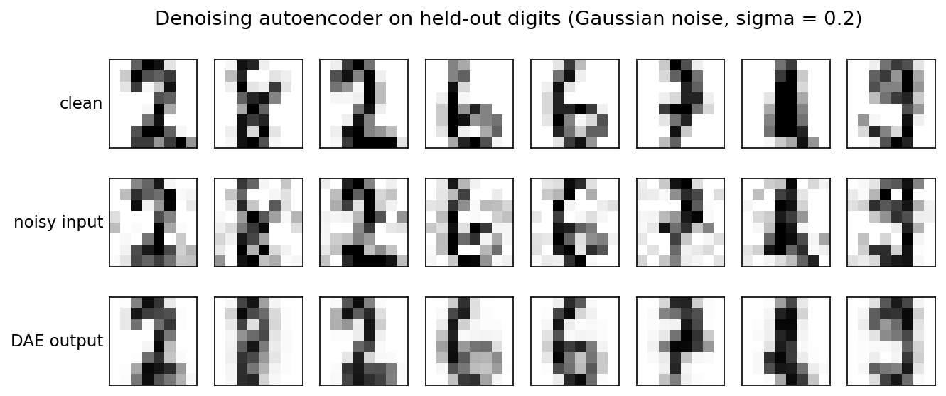
This standalone PyTorch example trains a small nonlinear DAE on training digits and evaluates clean reconstruction from noisy held-out input.
Code · Python · 23 lines
import torch
from torch import nn
from sklearn.datasets import load_digits
from sklearn.model_selection import train_test_split

torch.manual_seed(0); torch.set_num_threads(1)
train, test = train_test_split(load_digits().data/16., test_size=.2, random_state=0)
X = torch.tensor(train, dtype=torch.float32)
Xt = torch.tensor(test, dtype=torch.float32)
encoder = nn.Sequential(nn.Linear(64, 32), nn.ReLU(), nn.Linear(32, 12))
decoder = nn.Sequential(nn.Linear(12, 32), nn.ReLU(), nn.Linear(32, 64), nn.Sigmoid())
model = nn.Sequential(encoder, decoder)
opt = torch.optim.Adam(model.parameters(), lr=.003)
for step in range(2000):
    clean = X[torch.randint(len(X), (64,))]
    noisy = (clean + .2*torch.randn_like(clean)).clamp(0, 1)
    loss = (model(noisy)-clean).square().mean()
    opt.zero_grad(); loss.backward(); opt.step()
model.eval()
with torch.no_grad():
    noisy = (Xt + .2*torch.randn_like(Xt)).clamp(0, 1)
    print("noisy-input MSE:", (noisy-Xt).square().mean().item())
    print("reconstructed MSE:", (model(noisy)-Xt).square().mean().item())
Output (about 0.0248 for the noisy input and 0.0197 after the DAE; the last digits depend on the PyTorch build):
Code · 2 lines
noisy-input MSE: 0.024781296029686928
reconstructed MSE: 0.01968955807387829
The improvement is real but modest, and Figure 4 shows why: with a 12-dimensional code, the DAE removes the speckle but also smooths away some stroke detail. Denoising and faithful compression pull in different directions; a wider code or a convolutional architecture would shift the balance.
Contractive autoencoders
Plain version. A contractive penalty discourages large code changes under small input perturbations. It does not itself know which changes matter to the task.
Rifai et al. [12] add the squared Frobenius norm of the encoder’s Jacobian:
Here and the Jacobian entry measures how much code unit moves when input coordinate moves. For a single sigmoid layer , the entry is , so the penalty is cheap to compute:
The reconstruction term wants the code to change with the input (otherwise it could not reconstruct different inputs), while the penalty wants it to change as little as possible. The compromise is a code that is sensitive only along the few directions in which the training data actually vary. A DAE achieves a related effect implicitly: for small Gaussian noise, denoising training penalizes the sensitivity of the whole reconstruction function [1, ch. 14], whereas the CAE penalizes only the encoder, explicitly.
Code: the contractive penalty in action
Code · Python · 31 lines
import torch
from torch import nn
from sklearn.datasets import load_digits
from sklearn.model_selection import train_test_split

train, test = train_test_split(load_digits().data/16., test_size=.2, random_state=0)
X = torch.tensor(train, dtype=torch.float32)
Xt = torch.tensor(test, dtype=torch.float32)

def fit(lam):
    torch.manual_seed(0)
    W = nn.Linear(64, 16)                    # encoder h = sigmoid(Wx + b)
    dec = nn.Linear(16, 64)
    opt = torch.optim.Adam([*W.parameters(), *dec.parameters()], lr=3e-3)
    for step in range(1500):
        x = X[torch.randint(len(X), (64,))]
        h = torch.sigmoid(W(x))
        rec = (dec(h) - x).square().sum(1).mean()
        # ||J||_F^2 = sum_j (h_j(1-h_j))^2 * ||W_j||^2 for a sigmoid layer
        jac = ((h*(1-h))**2 * W.weight.square().sum(1)).sum(1).mean()
        loss = rec + lam*jac
        opt.zero_grad(); loss.backward(); opt.step()
    with torch.no_grad():
        h = torch.sigmoid(W(Xt))
        mse = (dec(h) - Xt).square().mean().item()
        jac = ((h*(1-h))**2 * W.weight.square().sum(1)).sum(1).mean().item()
    return mse, jac

for lam in (0.0, 0.5):
    mse, jac = fit(lam)
    print(f"lambda={lam}: test MSE={mse:.4f}, mean ||J||_F^2={jac:.2f}")
Output:
Code · 2 lines
lambda=0.0: test MSE=0.0141, mean ||J||_F^2=4.79
lambda=0.5: test MSE=0.0194, mean ||J||_F^2=0.70
The penalty cuts the encoder’s average sensitivity by a factor of almost seven, at the cost of a somewhat higher reconstruction error. Whether that trade is worthwhile depends on the downstream use: a smoother code often helps nearest-neighbor retrieval or classification with few labels, while a codec would prefer the unpenalized model.
The manifold view
Plain version. The manifold hypothesis models data near a lower-dimensional surface, like a rolled sheet in a room. Useful coordinates describe position along that surface.
The manifold hypothesis says that natural data, such as images, concentrate near a low-dimensional manifold embedded in the high-dimensional input space [3]. A random 64-pixel array almost never looks like a digit; the set of plausible digits is a tiny, structured region. Locally, around any data point, the manifold looks like a flat plane, the tangent space, spanned by the few directions you can move while staying realistic (thicker stroke, slight slant, small shift). Directions orthogonal to the tangent space lead off the manifold into noise.
This view gives a single lens for everything in the chapter:
- PCA fits one global flat sheet. It works when the manifold is nearly flat and fails when it is curved.
- Mixtures of PPCA or FA fit many local flat sheets.
- Nonlinear autoencoders learn a curved chart of the manifold: the encoder gives coordinates on the sheet, and the decoder maps them back into the room.
- Denoising teaches the model to move points that fell off the manifold back onto it.
- Contractive penalties make the encoder insensitive to directions orthogonal to the manifold, while reconstruction keeps it sensitive along the tangent directions [1, ch. 14], [12].
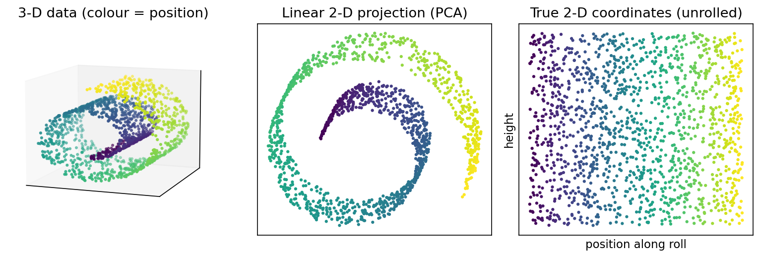
Figure 5 makes the limitation of linear methods concrete. The Swiss roll has two intrinsic dimensions, position along the roll and height, but no two-dimensional linear projection can unroll it: the PCA view keeps the spiral, so points far apart along the sheet are not laid out in order. A nonlinear encoder can, in principle, learn the unrolled coordinates. In practice, whether it does depends on capacity, regularization and the amount of data; manifold learning in high dimensions remains hard.
From autoencoders to VAEs
Plain version. An ordinary autoencoder learns to compress and decompress, but it gives no rule for inventing new codes. A VAE adds that rule.
Suppose a trained autoencoder maps every training digit to a code in . To generate a new digit, we would like to pick a random code and decode it. But which random code? The training codes may occupy a strange, clumpy region, and a random point between them may decode to garbage. Nothing in the reconstruction loss asked the code space to be smooth, filled, or shaped like any known distribution. Excellent reconstruction therefore does not imply good generation.
The variational autoencoder [13] fixes this by returning to the probabilistic factor-model story of PPCA and FA, but with a neural decoder:
where is a distribution whose parameters are produced by a decoder network. Because the true posterior is now intractable, a second network, the encoder, outputs an approximate posterior , typically a diagonal Gaussian. Training maximizes the evidence lower bound (ELBO) on :
Read the two terms against everything above:
- The reconstruction term is exactly an autoencoder loss, now with noise injected into the code. With a Gaussian decoder it becomes squared error, with a Bernoulli decoder binary cross-entropy.
- The KL term is a regularizer, like the sparse and contractive penalties, but chosen so that codes from all training examples together fill the prior. That is what makes sampling meaningful.
- With a linear Gaussian decoder, the model is PPCA. Its exact posterior is Gaussian and can be matched by a linear Gaussian encoder, so the bound becomes tight and the optimum coincides with the PPCA maximum-likelihood solution. The VAE is the nonlinear generalization of the factor models we began with.
Kingma and Welling’s introduction [14] develops this connection at length. Weighting the KL term by a factor gives the β-VAE [15], which was proposed to encourage disentangled factors at the cost of reconstruction quality; note that with the objective is no longer the ELBO. The full derivation of the ELBO, the reparameterization trick and failure modes such as posterior collapse are developed in ML 07.
What reconstruction error can and cannot tell you
Before leaving autoencoders, a practical warning. Reconstruction error is often used as an anomaly score: an autoencoder trained on normal data should reconstruct normal inputs well and unusual ones poorly. This can work, but it fails when the autoencoder generalizes too well and reconstructs unusual inputs too, or when anomalies differ only in fine detail that the bottleneck discards anyway. Similarly, a code that reconstructs well may be poor for classification, and a code that classifies well may discard the pixel detail a restoration task needs. Evaluate compression, denoising, downstream usefulness and generation separately.
Modern view
Plain version. The classical models of this chapter did not disappear. They became components: compression stages for generative models, pretraining objectives for vision, and microscopes for looking inside large networks.
Surveys worth reading
- Bengio, Courville and Vincent (2013) [3] is the standard review of representation learning. It frames good representations through a list of general priors (smoothness, multiple explanatory factors, a hierarchy of concepts, shared factors across tasks, the manifold hypothesis, sparsity and others), and connects autoencoders, probabilistic models and manifold learning under that lens. It is a good map for why the penalties in this chapter exist.
- Bank, Koenigstein and Giryes (2020) [16] is a compact survey chapter on autoencoders. It walks through regularized variants (sparse, denoising, contractive), VAEs and disentangled variants, applications (generative modeling, classification, clustering, anomaly detection, recommendation and dimensionality reduction) and hybrids with adversarial training, which makes it a useful companion to this tutorial.
- Kingma and Welling (2019) [14] is the authors’ own extended introduction to VAEs. It covers the ELBO, the reparameterization trick, richer posteriors and hierarchical models, and places VAEs among other deep latent-variable models.
- Goodfellow, Bengio and Courville [1, ch. 13–14] and Murphy [2] remain the clearest textbook treatments of linear factor models, the DAE–score connection and the manifold interpretation.
Disentanglement: a sober result
A recurring hope has been that unsupervised factor models would recover the true underlying factors, one per code unit (“disentanglement”). Locatello et al. [17] showed theoretically that unsupervised learning of disentangled representations is fundamentally impossible without inductive biases on both models and data, which mirrors the rotation ambiguity of factor analysis at a much larger scale. In a large reproducible study they also found that well-disentangled models could not be identified without supervision, and that more disentanglement did not reliably reduce the sample complexity of downstream tasks. The practical lesson echoes ICA: identifiability always comes from extra assumptions, so state them.
Autoencoders as tokenizers
The biggest modern role of autoencoders is as the first stage of large generative models. VQ-VAE [18] replaces the continuous code with a learned codebook of discrete vectors, so images become grids of discrete tokens that an autoregressive model can predict (see ML 09). Latent diffusion [19] trains an autoencoder for perceptual compression and then runs the diffusion model in its latent space instead of pixel space, which greatly reduces compute. In both cases, the autoencoder’s reconstruction quality sets a ceiling: the generator cannot restore detail the encoder discarded. Designing these tokenizers, balancing compression, reconstruction and how easy the latent space is for the generator to model, is an active research area as of 2026.
Sparse autoencoders for interpretability (2023–2026)
Sparse autoencoders have found a new and very active application: mechanistic interpretability of large language and vision models. The motivating observation is that individual neurons are often polysemantic, responding to several unrelated concepts. Cunningham et al. [20] trained overcomplete sparse autoencoders to reconstruct a language model’s internal activations, and found sparsely activating features that automated measures rated more interpretable and monosemantic than the neurons or other decompositions. Gao et al. [21] used -sparse (top-) autoencoders to control sparsity directly, reported clean scaling laws in autoencoder size and sparsity, proposed new metrics for feature quality, and trained a 16-million-latent autoencoder on GPT-4 activations. Conceptually this is sparse coding (Olshausen and Field’s idea) applied to a network’s activations instead of image patches.
Open problems
- Evaluation. Reconstruction error, sparsity and downstream accuracy disagree, and there is no agreed measure of whether learned features are the “right” ones, either for disentanglement or for interpretability.
- Identifiability. When can learned factors be trusted to correspond to real causes? Nonlinear ICA and causal representation learning study which extra assumptions (time structure, auxiliary variables, interventions) make this possible.
- Tokenizer design. How much to compress, whether codes should be discrete or continuous, and how to make latents both reconstructive and easy to model remain open engineering and theory questions.
Key takeaways
- Factor models explain observations through latent variables; their assumptions determine which representations are identifiable.
- PCA optimizes a linear reconstruction subspace; PPCA and factor analysis add different noise models.
- ICA, sparse coding and NMF use independence, sparsity and nonnegativity to favor different decompositions.
- A squared-error linear autoencoder can recover the PCA subspace at a suitable global optimum; its weights need not be PCA axes.
- Bottlenecks and sparse, denoising or contractive objectives constrain codes differently; reconstruction quality is not semantic quality.
- A VAE adds a probabilistic latent model and approximate inference; linear Gaussian choices connect it to PPCA.
Exercises
- Noise assumptions. You record 20 sensors, five of which are much noisier than the rest, but all respond to the same few underlying causes. Would you start with PPCA or factor analysis? What would PCA tend to do with the noisy sensors?
Hint
Factor analysis: its diagonal can assign large residual variance to the five noisy sensors without spending factors on them. PCA (and PPCA, with a single shared ) may devote components to the high-variance noisy sensors, because high variance is all PCA sees.
- Latent ambiguity. For an invertible matrix , show that replacing by and by leaves a linear autoencoder’s reconstruction unchanged. Which matrices also preserve the PPCA likelihood?
Hint
The product is . For PPCA, the likelihood depends on ; replacing by gives , which is unchanged when , that is, when is orthogonal.
- Why ICA fails on Gaussians. Generate two independent standard Gaussian sources, mix them with any invertible matrix, and run FastICA several times with different random seeds. What do you observe, and why?
Hint
After whitening, every rotation of two independent unit Gaussians is again two independent unit Gaussians, so there is no “right” rotation to find. Different seeds give different, equally valid unmixing directions, and the correlation with the true sources varies from run to run.
- Sparse codes versus PCA codes. Using the sparse-coding snippet, compare the number of nonzero code entries per test image with PCA codes of the same dimension (32). Then plot the test MSE of sparse coding as
alphavaries over 0.05, 0.1, 0.3, 1.0.
Hint
PCA codes are dense: essentially all 32 entries are nonzero. As alpha grows, the number of active atoms drops and the error rises, tracing a sparsity–fidelity curve. Remember that the dictionary was not given a mean term, so compare curves rather than single numbers with PCA.
- Denoising mismatch. Train the DAE from the tutorial on Gaussian noise, then test it on inputs where a random 3 × 3 block is set to zero. Then train a second DAE on that masking corruption and test both on both corruptions.
Hint
These are different corruption processes. The Gaussian-trained model has never been asked to fill in missing structure, so it typically leaves holes; the masking-trained model learns completion. Report a 2 × 2 table (train corruption × test corruption) rather than inferring robustness to one from success on the other.
- Contractive penalty by hand. For a single sigmoid unit , derive . When is it largest, and what does that say about where a contractive autoencoder allows its code to be sensitive?
Hint
, so the squared norm is . It is largest at (the steep middle of the sigmoid) and nearly zero when the unit is saturated. The penalty pushes units to be saturated for most inputs, keeping them in the sensitive regime only where the data require variation.
References
- I. Goodfellow, Y. Bengio and A. Courville, Deep Learning, MIT Press, 2016, ch. 13–14. Book
- K. P. Murphy, Probabilistic Machine Learning: An Introduction, MIT Press, 2022. Book
- Y. Bengio, A. Courville and P. Vincent, “Representation Learning: A Review and New Perspectives,” IEEE Transactions on Pattern Analysis and Machine Intelligence, vol. 35, no. 8, 2013. Paper
- M. E. Tipping and C. M. Bishop, “Probabilistic Principal Component Analysis,” Journal of the Royal Statistical Society: Series B, vol. 61, no. 3, 1999. Paper
- A. Hyvärinen and E. Oja, “Independent component analysis: algorithms and applications,” Neural Networks, vol. 13, no. 4–5, 2000. Paper
- B. A. Olshausen and D. J. Field, “Emergence of simple-cell receptive field properties by learning a sparse code for natural images,” Nature, vol. 381, 1996. Paper
- D. D. Lee and H. S. Seung, “Learning the parts of objects by non-negative matrix factorization,” Nature, vol. 401, 1999. Paper
- P. Baldi and K. Hornik, “Neural networks and principal component analysis: Learning from examples without local minima,” Neural Networks, vol. 2, no. 1, 1989. Paper
- G. E. Hinton and R. R. Salakhutdinov, “Reducing the Dimensionality of Data with Neural Networks,” Science, vol. 313, 2006. Paper
- P. Vincent, H. Larochelle, Y. Bengio and P.-A. Manzagol, “Extracting and composing robust features with denoising autoencoders,” ICML, 2008. Paper
- P. Vincent, H. Larochelle, I. Lajoie, Y. Bengio and P.-A. Manzagol, “Stacked Denoising Autoencoders: Learning Useful Representations in a Deep Network with a Local Denoising Criterion,” JMLR, vol. 11, 2010. Paper
- S. Rifai, P. Vincent, X. Muller, X. Glorot and Y. Bengio, “Contractive Auto-Encoders: Explicit Invariance During Feature Extraction,” ICML, 2011. Paper
- D. P. Kingma and M. Welling, “Auto-Encoding Variational Bayes,” ICLR, 2014. Paper
- D. P. Kingma and M. Welling, “An Introduction to Variational Autoencoders,” Foundations and Trends in Machine Learning, vol. 12, no. 4, 2019. Paper
- I. Higgins et al., “β-VAE: Learning Basic Visual Concepts with a Constrained Variational Framework,” ICLR, 2017. Paper
- D. Bank, N. Koenigstein and R. Giryes, “Autoencoders,” survey chapter, arXiv:2003.05991, 2020. Survey
- F. Locatello et al., “Challenging Common Assumptions in the Unsupervised Learning of Disentangled Representations,” ICML, 2019. Paper
- A. van den Oord, O. Vinyals and K. Kavukcuoglu, “Neural Discrete Representation Learning,” NeurIPS, 2017. Paper
- R. Rombach, A. Blattmann, D. Lorenz, P. Esser and B. Ommer, “High-Resolution Image Synthesis with Latent Diffusion Models,” CVPR, 2022. Paper
- H. Cunningham, A. Ewart, L. Riggs, R. Huben and L. Sharkey, “Sparse Autoencoders Find Highly Interpretable Features in Language Models,” arXiv:2309.08600, 2023. Paper
- L. Gao et al., “Scaling and evaluating sparse autoencoders,” arXiv:2406.04093, 2024. Paper
Check your understanding
This tutorial has 6 exercises. Can you solve them without opening the hints?
Go to the exercises ↑Next ML 07 · Generative Models: Autoencoders, VAEs, GANs and Flows · 29 min