ML 01A · Linear Algebra for Learning
Needs: ML 01 · Introduction to Machine Learning
Navigate: this page and this track: Navigate: this page and this track
On this page
- What you’ll learn1 min
- The big picture2 min
- Scalars, vectors, matrices and tensors2 min
- Multiplying matrices and vectors2 min
- Linear dependence, span and rank1 min
- Norms: measuring size2 min
- Special kinds of matrices and vectors1 min
- Eigendecomposition2 min
- Singular value decomposition3 min
- The Moore–Penrose pseudo-inverse3 min
- The trace operator1 min
- The determinant1 min
- Worked example: deriving principal component analysis3 min
- Matrix calculus you will meet1 min
- Modern view3 min
- Key takeaways1 min
- Exercises2 min
- Paper guides
- References
Machine Learning
Explore this chapter 1 interactive experiment
Move the images of the two basis vectors and watch a real photograph follow. The determinant is the signed area scale, the singular values are the stretch along two perpendicular directions, and rank 1 flattens the picture onto a line.
What you’ll learn
- Track array shapes and interpret matrix multiplication.
- Use rank, null spaces and norms to reason about linear systems.
- Read eigenvalues and singular values as geometric information.
- Solve least-squares problems and diagnose sensitivity to noise.
- Derive PCA and connect matrix identities to learning.
The big picture
Almost every operation inside a neural network is a linear map followed by a simple nonlinear function. A fully connected layer multiplies by a weight matrix. A convolution is a structured matrix product. Attention computes dot products between vectors and then mixes vectors with a matrix of weights. Linear algebra is the language for all of these. It tells us what a map keeps, what it throws away, what it stretches, and how to compute it without losing accuracy.
This chapter follows the “Applied Math” part of Goodfellow, Bengio and Courville’s Deep Learning [1] and the linear algebra chapters of Mathematics for Machine Learning [2]. Strang’s textbook [3] is the gentlest full course if you want more practice, and Golub and Van Loan [4] and Trefethen and Bau [5] are the standard references for how these computations are done reliably on a computer. Read this chapter before ML 02 if matrix notation is unfamiliar. The companion chapters are ML 01B · Probability and Information Theory and ML 01C · Numerical Computation.
The chapter has a single thread. We start with objects and shapes, move to products and solving equations, then measure size with norms. Eigendecomposition and the SVD then explain the “personality” of a matrix. The pseudo-inverse, trace and determinant are tools built on top of them. Finally, we use every one of these tools to derive PCA, the classic method for compressing data, exactly as it is derived in [1].
Scalars, vectors, matrices and tensors
Plain version. Every number in machine learning lives in an array with named axes. Name every axis before you multiply anything.
A scalar is a single number, written in italics: . A vector is an ordered list of numbers, written in bold lowercase or plain lowercase in this chapter: , with entries . By convention a vector is a column. A matrix is a 2-D grid of numbers: has rows and columns, and is the entry in row and column . A tensor is an array with any number of axes.
These objects map directly onto data:
- A grayscale image of height and width is a matrix in . Flattened, it becomes a vector . (See Images as Arrays.)
- A dataset of examples with features each, stored one example per row, is a design matrix .
- A fully connected layer with weights and bias maps the whole batch at once: , where is a vector of ones.
- An image batch in PyTorch is usually a 4-D tensor of shape (batch, channels, height, width). A batch of token embeddings in a Transformer is usually (batch, sequence length, embedding width).
The transpose swaps rows and columns: . It satisfies and . Note the reversed order.
Broadcasting
Writing is mathematically honest but tedious, so libraries let you add a vector to every row of a matrix directly. This is called broadcasting: when two arrays have different shapes, axes of length 1 (or missing leading axes) are stretched to match. Broadcasting is convenient and dangerous, because a wrong shape often still runs. The most common bug is subtracting a column vector of shape from a flat vector of shape , which silently produces an matrix instead of residuals.
Code · Python · 22 lines
import numpy as np

rng = np.random.default_rng(0)
X = rng.normal(size=(32, 64))      # batch of 32 examples, 64 features
W = rng.normal(size=(64, 10))      # linear map 64 -> 10
b = rng.normal(size=10)            # one bias per output
Y = X @ W + b                      # b broadcasts over the 32 rows
assert Y.shape == (32, 10)

# A classic broadcasting bug: (32,) - (32, 1) silently becomes (32, 32)
y_true = rng.normal(size=32)
y_pred = rng.normal(size=(32, 1))
print("buggy residual shape:", (y_true - y_pred).shape)
print("fixed residual shape:", (y_true - y_pred[:, 0]).shape)

# Four equivalent views of the same matrix product
A, B = rng.normal(size=(3, 4)), rng.normal(size=(4, 2))
entry = np.array([[A[i] @ B[:, j] for j in range(2)] for i in range(3)])
cols = np.stack([A @ B[:, j] for j in range(2)], axis=1)
outer = sum(np.outer(A[:, k], B[k]) for k in range(4))
assert np.allclose(A @ B, entry) and np.allclose(A @ B, cols) and np.allclose(A @ B, outer)
print("all views agree")
The output shows (32, 32) for the buggy line and (32,) for the fixed one. A mean over a array still returns a single number, so a loss computed this way trains without errors while optimizing the wrong thing. Put assert statements on shapes in any code you care about.
Multiplying matrices and vectors
Plain version. A matrix product chains two linear machines into one. Each output number is a dot product between a row of the first matrix and a column of the second.
For and , the matrix product is
Here indexes rows of (and of ), indexes columns of (and of ), and runs over the shared inner dimension . The inner dimensions must match; that is the first thing to check when a shape error appears.
The same product can be read in four ways, and each one is useful:
- Entry view. is the dot product of row of with column of . This is how attention scores are read: every query is compared with every key.
- Column view. Column of is times column of . Each column of is a combination of the columns of .
- Row view. Row of is row of times . In , each output example is its input row pushed through the same weights.
- Outer-product view. , a sum of rank-one matrices, each formed from column of and row of . This view explains low-rank approximation and LoRA later in the chapter.
The code above checks that all four views give the same answer.
Matrix multiplication is associative, , and distributive, , but not commutative: in general, and often one of the two products is not even defined. The elementwise (Hadamard) product multiplies matching entries instead and needs equal shapes. In NumPy and PyTorch, A @ B is the matrix product and A * B is elementwise. The dot product of two vectors is the special case , and it is symmetric: .
Identity, inverse and systems of equations
A system of linear equations in unknowns can be written compactly as
Each row of holds the coefficients of one equation, holds the unknowns, and holds the right-hand sides.
The identity matrix has ones on the diagonal and zeros elsewhere; it leaves every vector unchanged, . A square matrix is invertible if there is a matrix with . Then the system has exactly one solution, .
That formula is excellent for derivations and poor for computation. Explicitly forming costs more and loses more accuracy than solving the system directly with an LU, Cholesky or QR factorization [4], [5]. In NumPy, write np.linalg.solve(A, b), not np.linalg.inv(A) @ b. In this chapter, is a thinking tool.
Linear dependence, span and rank
Plain version. Rank counts how many genuinely different directions a matrix can produce. Repeated or redundant columns add nothing new.
A linear combination of vectors is for scalars . The span of a set of vectors is the set of all their linear combinations. Because , the vector is a linear combination of the columns of . So has a solution exactly when lies in the span of the columns, called the column space (or range) of .
A set of vectors is linearly independent if no vector in it is a linear combination of the others; equivalently, only when every . The rank of is the number of linearly independent columns, which always equals the number of linearly independent rows. For , ; if equality holds, has full rank.
The null space of is the set of vectors with . Those are the input directions that destroys. The rank–nullity theorem says
where is the number of columns and is the number of independent directions in the null space. This one equation explains the three regimes of :
| Shape and rank | What happens | Typical ML case |
|---|---|---|
| square, full rank | exactly one solution | a well-posed change of coordinates |
| tall (), full column rank | usually no exact solution; solve in the least-squares sense | regression with more examples than features |
| wide () or rank-deficient | infinitely many solutions (if any) | more parameters than constraints, as in deep networks |
For a square matrix, “invertible”, “full rank”, “columns linearly independent” and “null space contains only zero” are all the same statement. A square matrix that fails them is called singular.
Norms: measuring size
Plain version. A norm turns a vector into one non-negative number that says how big it is. Different norms disagree about what “big” means.
A norm is any function with , (the triangle inequality), and for every scalar . The most common family is the norm,
- , the Euclidean norm, is ordinary length; we often write . Its square is easier to differentiate and appears in mean-squared-error losses and weight decay.
- grows at the same rate everywhere, even near zero. That makes it useful when the difference between exactly zero and slightly nonzero matters, which is why penalties encourage sparse solutions.
- , the max norm, is the size of the largest entry. Adversarial-robustness work often bounds perturbations in this norm.
- The count of nonzero entries is sometimes called the ” norm”, but it is not a norm: scaling by 2 does not change it.
The dot product connects to the Euclidean norm through angles: , where is the angle between and . The cosine similarity
is defined for nonzero vectors and ignores scale. That is useful for some embeddings (contrastive learning normalizes features for this reason) and wrong when magnitude carries meaning, such as image brightness.
Matrix norms
For matrices we use two norms constantly. The Frobenius norm treats the matrix as one long vector,
The spectral norm (operator 2-norm) measures the largest factor by which can stretch a unit vector,
where is the largest singular value, defined in the SVD section below. In terms of all singular values , we have while . So many small singular values can make the Frobenius norm large without changing the largest amplification. The spectral norm bounds how much a layer can magnify a perturbation of its input, which is why it appears in robustness and GAN-stability work [17].
Code · Python · 13 lines
import numpy as np

x = np.array([3.0, -4.0, 0.0, 1.0])
for p in [1, 2, np.inf]:
    print(f"L{p} norm:", np.linalg.norm(x, p))
print("L0 'norm' (count of nonzeros):", np.count_nonzero(x))

A = np.array([[3.0, 0.0], [4.0, 5.0]])
s = np.linalg.svd(A, compute_uv=False)
print("singular values:", s.round(4))
print("Frobenius:", np.linalg.norm(A, "fro"), "=", np.sqrt((s**2).sum()))
print("spectral :", np.linalg.norm(A, 2), "=", s[0])
assert np.isclose(np.linalg.norm(A, "fro")**2, np.trace(A.T @ A))
For this prints , , and three nonzeros. For the matrix the singular values are and , giving and .
Special kinds of matrices and vectors
Plain version. Some matrices are much easier to work with than others. Learning to spot them saves computation and explains many design choices.
- A diagonal matrix has nonzero entries only on its main diagonal. Multiplying by it scales each coordinate: . Its inverse, when every , is . Per-channel scaling in normalization layers is a diagonal matrix in disguise. Rectangular diagonal matrices also exist; they appear in the SVD.
- A symmetric matrix satisfies . Covariance matrices, Gram matrices , Hessians of smooth functions and distance matrices are symmetric.
- A unit vector has . Two vectors are orthogonal if ; if they are also unit vectors, they are orthonormal.
- An orthogonal matrix is square with orthonormal rows and columns, so and . Its inverse is free to compute. It preserves lengths and angles, , so geometrically it is a rotation, a reflection, or both.
If has orthonormal columns, then but . The matrix is the orthogonal projection onto the span of the columns of . The projection is the closest point to in that subspace, and the residual is perpendicular to every column of . Projecting twice changes nothing: . PCA, below, is exactly the search for the best such .
Eigendecomposition
Plain version. A real eigenvector stays on the same line after transformation. Its eigenvalue sets the scale and may reverse its direction.
An eigenvector of a square matrix is a nonzero vector with
where the scalar is the corresponding eigenvalue. If is an eigenvector, so is for any , so we usually normalize eigenvectors to unit length.
Suppose has linearly independent eigenvectors with eigenvalues . Stack them as columns of and put the eigenvalues in . Then , so
This is the eigendecomposition. It says: change to eigenvector coordinates (), scale each coordinate independently (), and change back (). Not every matrix has one. The shear has only one independent eigenvector. A rotation by has eigenvalues , which are complex, because no real direction is left unturned.
The symmetric case
Symmetric matrices are the friendly case, and they are the ones ML meets most. The spectral theorem says that every real symmetric matrix can be written as
where is orthogonal (its columns are orthonormal eigenvectors) and is real and diagonal [3], [4]. Because , no inversion is needed. Geometrically, stretches space by along the direction , the -th column of . The decomposition is unique up to the order of the eigenvalues and the choice of basis within any repeated eigenvalue; by convention we sort eigenvalues from largest to smallest.
For a symmetric , the quadratic form restricted to unit vectors is bounded by the extreme eigenvalues:
with the maximum reached at the top eigenvector and the minimum at the bottom one. The ratio is called the Rayleigh quotient. This fact is the engine of the PCA derivation later.
Positive definite matrices
The signs of the eigenvalues classify symmetric matrices:
| Name | Eigenvalues | Equivalent condition |
|---|---|---|
| positive definite (PD) | all | for every |
| positive semidefinite (PSD) | all | for every |
| negative (semi)definite | all (or ) | the reverse inequalities |
| indefinite | both signs present | takes both signs |
Every covariance matrix and every Gram matrix is PSD, because . A Gaussian density needs a PD covariance so that it can be inverted. The Hessian of a loss is PD at a strict local minimum and indefinite at a saddle point; ML 01C uses this to explain why optimization can be slow. A PD matrix has a Cholesky factorization with lower triangular, which is the fastest stable way to solve systems with it and to sample from a Gaussian [4].
Code · Python · 17 lines
import numpy as np

rng = np.random.default_rng(1)
M = rng.normal(size=(4, 4))
S = M @ M.T + 0.1 * np.eye(4)        # symmetric positive definite
lam, Q = np.linalg.eigh(S)           # ascending eigenvalues, orthonormal Q
assert np.allclose(Q @ np.diag(lam) @ Q.T, S)
assert np.allclose(Q.T @ Q, np.eye(4))
print("eigenvalues:", lam.round(3), "all positive:", bool((lam > 0).all()))

# The quadratic form x^T S x is bounded by the extreme eigenvalues
x = rng.normal(size=4); x /= np.linalg.norm(x)
print("Rayleigh quotient in range:", lam[0] <= x @ S @ x <= lam[-1])

# A non-symmetric matrix can have complex eigenvalues
R = np.array([[0.0, -1.0], [1.0, 0.0]])  # 90-degree rotation
print("rotation eigenvalues:", np.linalg.eigvals(R))
Use np.linalg.eigh for symmetric matrices: it is faster, returns real eigenvalues in ascending order and orthonormal eigenvectors. np.linalg.eig handles the general case and may return complex numbers, as the rotation shows.
Singular value decomposition
Plain version. SVD decomposes a real matrix into orthogonal changes of coordinates and axis-wise scaling. Those coordinate changes may include reflections.
Eigendecomposition needs a square matrix and may not exist. The singular value decomposition always exists, for every real matrix :
- is orthogonal. Its columns are the left singular vectors, directions in the output space.
- is rectangular diagonal. Its diagonal entries are the singular values.
- is orthogonal. Its columns are the right singular vectors, directions in the input space.
Read from right to left, first expresses in the coordinates (a rotation or reflection), then scales coordinate by , then places the result along the directions. Figure 1 shows this for a matrix: the unit circle becomes an ellipse whose semi-axes have lengths and .
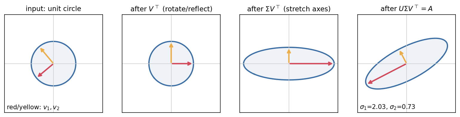
The SVD and eigendecomposition are closely related. Since and , the right singular vectors are eigenvectors of , the left singular vectors are eigenvectors of , and . For a symmetric PSD matrix, the SVD and the eigendecomposition coincide.
The number of nonzero singular values equals the rank . Keeping only those gives the compact (thin) SVD , a sum of rank-one matrices. That is the outer-product view of a matrix product again.
The best low-rank approximation
Truncating that sum after terms gives . The Eckart–Young theorem [6] says that is the best rank- approximation of in the Frobenius norm:
The same is also optimal in the spectral norm, with error [4]. In words: throw away the smallest singular values, and the energy you lose is exactly what you threw away. Storing needs numbers instead of .
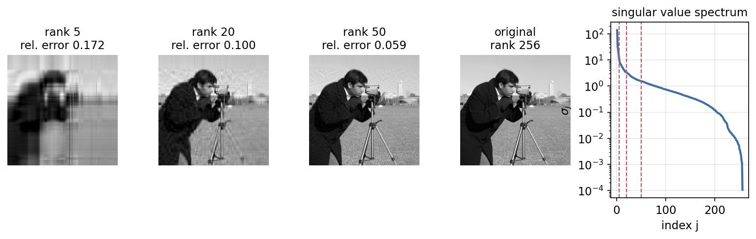
Figure 2 applies this to a grayscale photograph. Natural images have rapidly decaying singular values, so a rank-50 approximation already keeps the main structure. The streaky artifacts at low rank come from the fact that each rank-one term is an outer product of a column pattern and a row pattern.
Code · Python · 16 lines
import numpy as np

rng = np.random.default_rng(0)
A = rng.normal(size=(12, 8))
U, s, Vt = np.linalg.svd(A, full_matrices=False)
assert np.allclose(U @ np.diag(s) @ Vt, A)
k = 3
Ak = (U[:, :k] * s[:k]) @ Vt[:k]
err_F = np.linalg.norm(A - Ak, "fro")**2
err_2 = np.linalg.norm(A - Ak, 2)
assert np.isclose(err_F, (s[k:]**2).sum()) and np.isclose(err_2, s[k])
print("rank-k squared Frobenius error:", round(err_F, 3))
print("rank-k spectral error = sigma_{k+1}:", round(err_2, 3), round(s[k], 3))
# Eigenvalues of A^T A are squared singular values of A
assert np.allclose(np.sort(np.linalg.eigvalsh(A.T @ A))[::-1], s**2)
print("storage: full", A.size, "numbers; rank-3 factors", k * (12 + 8 + 1))
full_matrices=False returns the thin SVD, which is what you almost always want. (U[:, :k] * s[:k]) scales the columns of by broadcasting instead of building a diagonal matrix. Both Eckart–Young identities hold to machine precision.
One caveat: the directions with the largest singular values carry the most energy, not necessarily the most useful information. For classification, a small-variance direction can be the one that separates the classes. PR 05 contrasts PCA with discriminant methods for exactly this reason.
The Moore–Penrose pseudo-inverse
Plain version. When a matrix has no inverse, the pseudo-inverse gives the next best thing: the answer that fits the data as closely as possible, and among equally good answers, the smallest one.
Only square, full-rank matrices have inverses. For any , the Moore–Penrose pseudo-inverse is the unique matrix satisfying the four Penrose conditions [7]:
It is easiest to compute from the SVD. If , then
where is formed by transposing and replacing each nonzero singular value by (zeros stay zero). Goodfellow et al. give the equivalent limit [1], which already hints at ridge regression.
The pseudo-inverse gives the right answer in every regime of the rank table:
- Tall, full column rank (). usually has no exact solution. Then is the least-squares solution: it minimizes .
- Wide, full row rank (). There are infinitely many solutions. Then is the solution with the smallest , the minimum-norm solution. Any other solution adds a null-space vector, which can only increase the norm.
- Rank-deficient. is both: among all least-squares minimizers, the one with the smallest norm.
The minimum-norm property is a small window into a modern question. Gradient descent on an under-determined least-squares problem, started from zero, converges to the minimum-norm solution, because every gradient lies in the row space of . Over-parameterized networks are not linear, but this simple case is the usual starting point for thinking about which of many perfect fits a training algorithm picks.
Least squares, the normal equations and conditioning
For a regression design matrix and targets , least squares minimizes . Setting the gradient to zero gives the normal equations
These are correct but numerically risky. The sensitivity of a linear problem is measured by the condition number . Roughly, relative errors in the data can be amplified by up to a factor in the solution [5]. Forming squares the condition number, , so a mildly ill-conditioned problem becomes a severely ill-conditioned one. Library least-squares solvers (np.linalg.lstsq, torch.linalg.lstsq) work with QR or SVD factorizations of directly and avoid that squaring [4].
When two features are almost identical, is tiny, and the individual coefficients become extremely sensitive even when predictions are fine. Ridge regression [8] adds a penalty with :
The SVD form on the right shows what ridge does. Plain least squares uses the factor , which explodes for small . Ridge uses , which stays bounded by . Large- directions are nearly untouched; small- directions are suppressed. The price is bias. In neural networks the same penalty is called weight decay.
Code · Python · 28 lines
import numpy as np

rng = np.random.default_rng(0)
# Over-determined: more equations than unknowns -> least squares
x = np.linspace(-1, 1, 40)
X = np.c_[np.ones_like(x), x]
y = 2 + 3*x + rng.normal(0, .05, len(x))
w, residuals, rank, sv = np.linalg.lstsq(X, y, rcond=None)
print("intercept and slope:", w.round(3), "rank:", rank)
assert np.allclose(w, np.linalg.pinv(X) @ y)

# Under-determined: fewer equations than unknowns -> minimum-norm solution
A = rng.normal(size=(2, 5)); b = rng.normal(size=2)
w_min = np.linalg.pinv(A) @ b
null = np.linalg.svd(A)[2][-1]             # a direction with A @ null = 0
w_other = w_min + 0.7 * null
print("both solve Aw=b:", np.allclose(A @ w_min, b), np.allclose(A @ w_other, b))
print("norms:", np.linalg.norm(w_min).round(3), "<", np.linalg.norm(w_other).round(3))

# Near-collinear features: condition number and ridge
z = rng.normal(size=200)
F = np.c_[z, z + 1e-4 * rng.normal(size=200)]
t = z + 0.01 * rng.normal(size=200)
print("cond(F) = %.1e, cond(F^T F) = %.1e" % (np.linalg.cond(F), np.linalg.cond(F.T @ F)))
w_ls = np.linalg.lstsq(F, t, rcond=None)[0]
lam = 1e-2
w_ridge = np.linalg.solve(F.T @ F + lam * np.eye(2), F.T @ t)
print("least squares:", w_ls.round(2), " ridge:", w_ridge.round(3))
The line fit recovers intercept and slope , and pinv agrees with lstsq. The under-determined system has two exact solutions; the pseudo-inverse one has the smaller norm (0.885 versus 1.128). In the collinear case, while , its square. Least squares returns wild coefficients whose sum is still about 1, so its predictions are fine. Ridge returns the stable split . The intercept column in the first example lets the line have a nonzero offset. In a real pipeline, fit any centering and scaling on the training set only, then apply it unchanged to validation and test data.
The trace operator
Plain version. The trace adds up the diagonal. It looks too simple to matter, but it lets you rewrite awkward sums as matrix expressions and move matrices around inside them.
The trace of a square matrix is
Its useful properties are:
- Frobenius norm. .
- Transpose. .
- Cyclic property. whenever the products are defined, even when the matrices are not square and the intermediate products have different shapes. In particular for , . You may cycle, but not arbitrarily reorder: in general.
- Scalars. A scalar is its own trace, . This turns a quadratic form into a trace: .
- Eigenvalues. . For a covariance matrix, that is the total variance, the sum of the variances along every principal direction.
The scalar trick is how many expectations are evaluated. For a random vector with mean zero and covariance , , because trace and expectation are both linear.
The determinant
Plain version. The absolute determinant gives volume scaling; its sign records orientation. A zero determinant means a square matrix collapses a dimension and is not invertible.
The determinant of a square matrix is a single number with these properties:
- , the product of the eigenvalues.
- is the factor by which scales volume. The unit cube maps to a parallelepiped of volume .
- The sign records orientation. A negative determinant means includes a reflection.
- exactly when is singular: some direction is collapsed to zero, so information is lost.
- , , and .
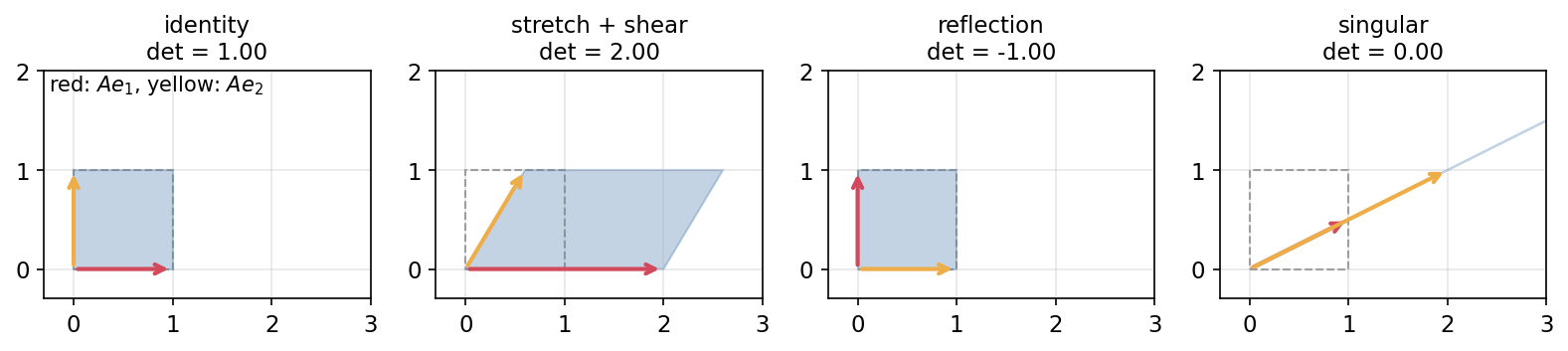
Determinants appear in machine learning in two main places. The multivariate Gaussian density contains , the volume normalization of the covariance; ML 01B uses it. Normalizing flows (ML 07) need of a Jacobian matrix to account for how an invertible network stretches probability mass. In both cases you need the logarithm, never the raw value: the determinant of a diagonal matrix with entries is , which underflows to zero in float64.
Code · Python · 19 lines
import numpy as np

rng = np.random.default_rng(2)
A, B, C = rng.normal(size=(3, 4)), rng.normal(size=(4, 5)), rng.normal(size=(5, 3))
print("cyclic trace:", np.isclose(np.trace(A @ B @ C), np.trace(C @ A @ B)),
      np.isclose(np.trace(A @ B @ C), np.trace(B @ C @ A)))

S = rng.normal(size=(4, 4))
lam = np.linalg.eigvals(S)
print("trace = sum of eigenvalues:", np.isclose(np.trace(S), lam.sum().real))
print("det = product of eigenvalues:", np.isclose(np.linalg.det(S), np.prod(lam).real))

# log-determinant of a covariance without overflow/underflow
Sigma = np.diag(np.full(500, 1e-3))
print("det underflows:", np.linalg.det(Sigma))
sign, logdet = np.linalg.slogdet(Sigma)
print("slogdet:", sign, round(logdet, 2))
L = np.linalg.cholesky(Sigma)
print("via Cholesky:", round(2 * np.log(np.diag(L)).sum(), 2))
The direct determinant prints 0.0, while slogdet and the Cholesky route both give . For a PD matrix, when , so .
Worked example: deriving principal component analysis
Plain version. PCA looks for the flat subspace that the data cloud lies closest to. Projecting onto it compresses each point to a few numbers while losing as little as possible.
PCA goes back to Pearson’s “lines and planes of closest fit” [9] and Hotelling’s analysis of “principal components” [10]; Jolliffe and Cadima give a modern review [11]. We derive it in the style of [1], using only the tools above.
Setup. We have points and want to store each one with only numbers. First subtract the mean from every point, so we can assume the data are centered. Stack the centered points as rows of .
Step 1: choose the form of the code. We use a linear decoder with . To make the problem well-posed we require the columns of to be orthonormal, . (Without this, we could shrink and enlarge forever.)
Step 2: find the best code for a fixed decoder. For a given , choose to minimize the reconstruction error:
We expanded the square, dropped (it does not depend on ) and used . The gradient with respect to is . Setting it to zero gives the encoder
So encoding is a matrix–vector product, and the reconstruction is , the orthogonal projection of onto the span of .
Step 3: find the best decoder. Now choose to minimize the total reconstruction error over all points:
Start with , so is a single unit vector . Write the Frobenius norm as a trace and expand:
The cyclic property moved to the front in the second and third terms, and simplified the last line. The first term does not depend on . So minimizing the error is the same as
That is a Rayleigh quotient of the symmetric PSD matrix . By the eigendecomposition section, it is maximized by the eigenvector of with the largest eigenvalue.
Step 4: more than one component. Repeating the argument for general (for example, by induction, requiring each new direction to be orthogonal to the previous ones) gives the answer: the columns of are the eigenvectors of for the largest eigenvalues [1]. The minimum error equals the sum of the discarded eigenvalues.
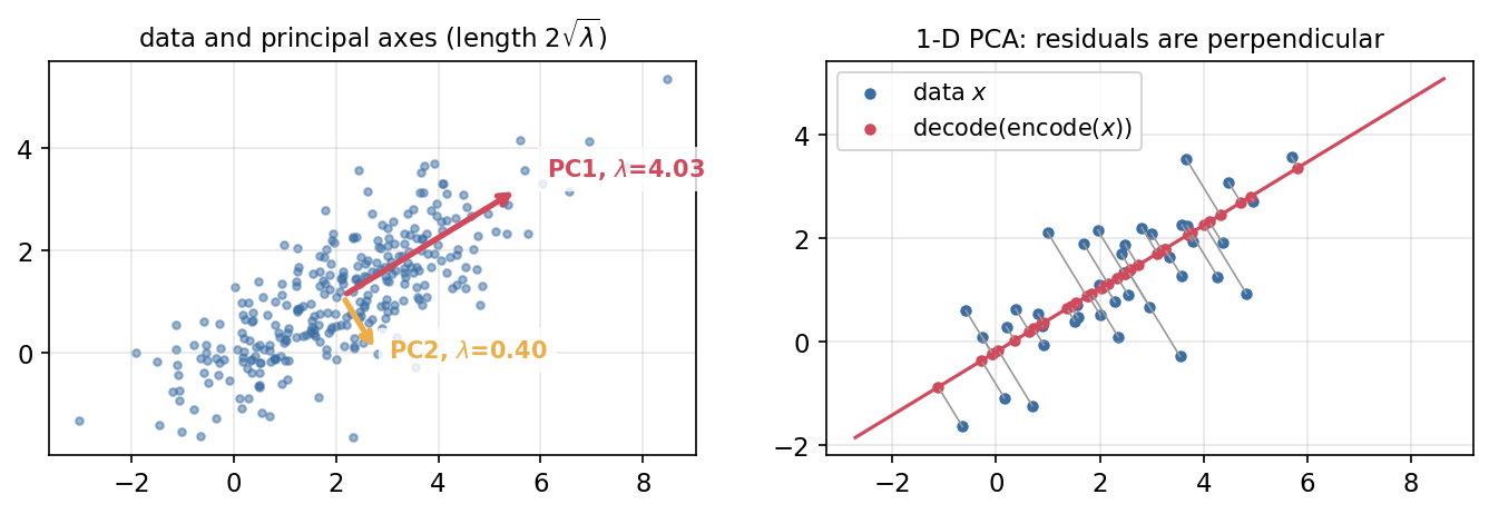
Step 5: the variance view and the SVD link. Dividing by turns into the sample covariance (some texts use ). The quantity is the variance of the projected data . So “minimize reconstruction error” and “maximize retained variance” select the same directions: Pearson’s and Hotelling’s views agree. Finally, if the centered data matrix has thin SVD , then . The principal directions are the right singular vectors , the eigenvalues are , and the codes are . In practice PCA is computed with the SVD of rather than by forming the covariance, for the conditioning reason we met in least squares.
Code · Python · 26 lines
import numpy as np

rng = np.random.default_rng(0)
n, d, l = 500, 5, 2
Z = rng.normal(size=(n, l))
X = Z @ rng.normal(size=(l, d)) + 0.1 * rng.normal(size=(n, d)) + 3.0

mu = X.mean(axis=0)
Xc = X - mu                                  # centre first
S = Xc.T @ Xc / n                            # sample covariance (d x d)
lam, Q = np.linalg.eigh(S)
lam, Q = lam[::-1], Q[:, ::-1]               # descending
D = Q[:, :l]                                 # decoder matrix, orthonormal columns

codes = Xc @ D                               # encode: f(x) = D^T (x - mu)
X_hat = codes @ D.T + mu                     # decode: g(c) = D c + mu
mse = np.mean(np.sum((X - X_hat)**2, axis=1))
print("explained variance ratio:", (lam[:l].sum() / lam.sum()).round(4))
print("reconstruction MSE:", mse.round(5), " sum of discarded eigenvalues:", lam[l:].sum().round(5))
assert np.isclose(mse, lam[l:].sum())

# Same subspace from the SVD of the centred data matrix
U, s, Vt = np.linalg.svd(Xc, full_matrices=False)
assert np.allclose(s[:l]**2 / n, lam[:l])
assert np.allclose(np.abs(Vt[:l] @ D), np.eye(l), atol=1e-8)
print("SVD and eigendecomposition agree")
The synthetic data are 5-D points that really live near a 2-D plane, plus small noise. Two components explain 99.36% of the variance, and the average squared reconstruction error equals the sum of the three discarded eigenvalues, exactly as Step 4 predicts. The SVD route finds the same directions (up to sign, which is arbitrary for eigenvectors).
Three practical notes. Always center the data, or the first “component” just points at the mean. Standardize features if they have incomparable units, because PCA is not scale-invariant. And fit the mean and directions on training data only. PCA is the linear ancestor of autoencoders; ML 06A develops the probabilistic version and its nonlinear successors.
Optional: PCA (in the Paper guides). Read the original figure, evidence, design choices and limitations.
Matrix calculus you will meet
Plain version. Training means following gradients, and most gradients in ML are a handful of matrix formulas used over and over.
For a scalar function of a vector , the gradient collects the partial derivatives . For a vector function , the Jacobian has entries . The rules you will use most are:
| Function | Gradient | Note |
|---|---|---|
| linear function | ||
| becomes when is symmetric | ||
| least-squares loss | ||
| weight decay | ||
| w.r.t. | used with the trace tricks above |
Each can be verified by writing the expression as a sum over indices and differentiating term by term [2]. The chain rule for vector functions multiplies Jacobians: if and is a scalar, then . Backpropagation applies this rule layer by layer, multiplying transposed local Jacobians by the incoming gradient without ever building the full Jacobians, which would be enormous. ML 02 builds this up in detail, and ML 01C adds the Hessian, the matrix of second derivatives.
Setting the least-squares gradient to zero recovers the normal equations from the previous section. The Hessian of that loss is , which is PSD, so the loss is convex and every stationary point is a global minimum. A quick finite-difference check confirms the formula:
Code · Python · 13 lines
import numpy as np

rng = np.random.default_rng(3)
X, y = rng.normal(size=(30, 4)), rng.normal(size=30)
w = rng.normal(size=4)
L = lambda w: 0.5 * np.sum((X @ w - y)**2)
grad = X.T @ (X @ w - y)                    # analytic gradient
eps = 1e-6
num = np.array([(L(w + eps*e) - L(w - eps*e)) / (2*eps) for e in np.eye(4)])
print("max gradient mismatch:", np.abs(grad - num).max())
# Setting the gradient to zero gives the normal equations
w_star = np.linalg.lstsq(X, y, rcond=None)[0]
print("gradient at solution ~ 0:", np.abs(X.T @ (X @ w_star - y)).max() < 1e-10)
The analytic and numerical gradients agree to about , the size expected from finite-difference rounding.
Modern view
The definitions in this chapter are a century old, but the way they are used in machine learning keeps changing. Four lines of work are worth knowing about.
Randomized numerical linear algebra. Exact SVDs of large matrices are expensive, roughly operations. Halko, Martinsson and Tropp’s SIAM Review survey [12] made a simple idea standard: multiply by a thin random matrix to “sketch” its range, orthonormalize the result to get a basis , and compute an exact SVD of the small matrix . With a little oversampling and a few power iterations, the result is accurate for matrices whose spectrum decays. Martinsson and Tropp’s Acta Numerica survey [13] covers the theory and a wide range of algorithms: norm estimation, random embeddings, regression, low-rank approximation, Nyström approximation of PSD matrices, streaming algorithms and kernel matrices from machine learning. Murray et al. [14] (LAPACK Working Note 299, 2023) take the software view. They note that RandNLA methods have entered MATLAB, the NAG Library, NVIDIA’s cuSOLVER and scikit-learn, and they argue for standard “RandBLAS” and “RandLAPACK” libraries. scikit-learn’s randomized PCA solver is a direct descendant. The core algorithm fits in a few lines:
Code · Python · 21 lines
import numpy as np

def randomized_svd(A, k, oversample=10, power_iters=2, seed=0):
    rng = np.random.default_rng(seed)
    Omega = rng.normal(size=(A.shape[1], k + oversample))  # random test matrix
    Y = A @ Omega                                          # sample the range of A
    for _ in range(power_iters):                           # sharpen a slow spectrum
        Y = A @ (A.T @ Y)
    Q, _ = np.linalg.qr(Y)                                 # orthonormal basis
    B = Q.T @ A                                            # small (k+p) x n matrix
    Ub, s, Vt = np.linalg.svd(B, full_matrices=False)
    return (Q @ Ub)[:, :k], s[:k], Vt[:k]

rng = np.random.default_rng(1)
m, n, r = 2000, 500, 20
A = rng.normal(size=(m, r)) @ rng.normal(size=(r, n)) + 0.01 * rng.normal(size=(m, n))
U, s, Vt = randomized_svd(A, k=r)
s_exact = np.linalg.svd(A, compute_uv=False)[:r]
print("max relative error in top singular values:", np.max(np.abs(s - s_exact) / s_exact))
rel = np.linalg.norm(A - (U * s) @ Vt) / np.linalg.norm(A)
print("relative reconstruction error:", round(rel, 5))
On this nearly rank-20 matrix the top 20 singular values match the exact ones to about relative error, and the rank-20 reconstruction error (about 0.2%) is set by the added noise. The power iterations are what make it work when the spectrum decays slowly. For a matrix with a flat spectrum, no rank- method can do well, randomized or not.
Low-rank structure in large models. The outer-product view of matrix products has become a practical tool for adapting large networks. LoRA [15] freezes a pretrained weight and learns an update with , and . Only numbers are trained instead of ; for and , that is 65,536 instead of about 16.8 million per matrix. starts at zero, so training begins exactly at the pretrained model. GaLore [16] (ICML 2024) keeps all weights trainable but projects the gradients onto a low-rank subspace, which shrinks the optimizer’s memory. Its authors argue that restricting the weight update itself to a low-rank subspace, as LoRA does, can underperform full-rank training. Both rely on the Eckart–Young intuition that much of a matrix’s useful content lives in a few singular directions. Whether that holds for a given task is an empirical question, not a theorem.
Controlling the spectral norm. A network’s sensitivity to input perturbations is bounded by the product of its layers’ spectral norms (for 1-Lipschitz activations such as ReLU). Spectral normalization [17] divides each weight matrix by an estimate of its largest singular value, obtained cheaply with one step of power iteration per training step. It was introduced to stabilize the discriminator in GANs (ML 07), and the same idea appears wherever a Lipschitz bound is wanted.
Beyond matrices. Convolution kernels and video features are naturally tensors with three or more axes. Kolda and Bader’s SIAM Review survey [18] is the standard introduction to tensor decompositions. It covers the CP decomposition (a sum of rank-one tensors, generalizing the outer-product view) and the Tucker decomposition (a small core tensor multiplied by a matrix along each mode, generalizing the SVD). Unlike matrices, computing the rank of a tensor is hard in general, and best low-rank approximations need not exist. The clean Eckart–Young picture does not carry over. These decompositions are used to compress layers and to analyze multi-way data.
Open questions. Why do trained weight matrices often have rapidly decaying spectra, and how does that relate to generalization? How low can the rank of an adaptation be before quality drops, and does that depend on the task or the model? How should randomized algorithms be combined with low-precision hardware, where rounding errors are much larger than in float64? None of these have settled answers. The tools in this chapter are what you need to read the papers that study them. For broader textbook treatments that connect linear algebra to deep learning, see [1], [2] and [19].
Key takeaways
- Name each axis and check shapes before multiplying or broadcasting arrays.
- Rank and null space constrain possible solutions; use a linear solver instead of explicitly inverting a matrix to solve a system.
- Real symmetric matrices admit an orthonormal eigenbasis; eigenvalue signs describe their quadratic forms.
- Truncated SVD gives a best low-rank approximation under spectral or Frobenius error.
- The pseudo-inverse selects the minimum-norm least-squares solution; small singular values can amplify noise.
- PCA on centered data maximizes retained variance and minimizes squared reconstruction error for a fixed subspace dimension.
Exercises
- Shapes and bias. A batch has shape and a weight matrix has shape . What shape should the bias have, and what goes wrong if you use a bias of shape instead?
Hint
A bias of shape broadcasts over the 32 rows: one offset per output unit, shared by every example. A bias broadcasts across the 10 columns, giving one offset per example. The code runs, but the “bias” now depends on the position of an example in the batch, which is meaningless and changes with batch size.
- Projection. Let have orthonormal columns and . Show that , , and that is orthogonal to every column of . What are the eigenvalues of ?
Hint
. For orthogonality compute . From , any eigenvalue satisfies , so : eigenvalue 1 with multiplicity (the subspace) and 0 with multiplicity (its orthogonal complement). Hence .
- SVD by hand. Find the singular values of by computing the eigenvalues of . Check that and .
Hint
has eigenvalues and , so , . Then , and . In general for a square matrix, because .
- Conditioning and ridge. Starting from the least-squares code, replace the second feature by an exact copy of the first. What does
np.linalg.lstsqreturn, and why is it the minimum-norm solution? Then derive the SVD form of the ridge solution and show that each factor is at most .
Hint
With identical columns, the rank is 1 and the solution set is a line . lstsq uses the SVD and returns the pseudo-inverse solution, which splits the weight equally, , because that point on the line is closest to the origin. For the bound, maximize : at , giving .
- PCA error. Using the derivation in this chapter, show that the total reconstruction error of -component PCA equals , and that the fraction of variance retained is . Then run PCA on
sklearn.datasets.load_digits()and find the smallest that keeps 90% of the variance.
Hint
Write (use and the cyclic property). With the top- eigenvectors, the second trace is , and . For the digits, center the matrix, compute its singular values, and take the cumulative sum of . Report your own number rather than trusting a quoted one.
- Determinants and volume. A matrix maps the unit square to a parallelogram with vertices , , and . Write down a matrix that does this, compute its determinant, and explain why a normalizing flow must track for every layer.
Hint
Put the edge vectors in the columns: , with , so areas grow by a factor of 5. If a map stretches volume by 5, probability density must shrink by the same factor to keep total probability equal to 1. Stacking layers multiplies these factors, so their logarithms add, which is why flows sum log-determinants layer by layer.
References
- I. Goodfellow, Y. Bengio and A. Courville, Deep Learning, MIT Press, 2016, ch. 2 “Linear Algebra”. Book
- M. P. Deisenroth, A. A. Faisal and C. S. Ong, Mathematics for Machine Learning, Cambridge University Press, 2020. Book
- G. Strang, Introduction to Linear Algebra, 6th ed., Wellesley-Cambridge Press, 2023. Book site
- G. H. Golub and C. F. Van Loan, Matrix Computations, 4th ed., Johns Hopkins University Press, 2013. DOI
- L. N. Trefethen and D. Bau III, Numerical Linear Algebra, SIAM, 1997. DOI
- C. Eckart and G. Young, “The Approximation of One Matrix by Another of Lower Rank,” Psychometrika, vol. 1, pp. 211–218, 1936. DOI
- R. Penrose, “A Generalized Inverse for Matrices,” Mathematical Proceedings of the Cambridge Philosophical Society, vol. 51, pp. 406–413, 1955. DOI
- A. E. Hoerl and R. W. Kennard, “Ridge Regression: Biased Estimation for Nonorthogonal Problems,” Technometrics, vol. 12, pp. 55–67, 1970. DOI
- K. Pearson, “On Lines and Planes of Closest Fit to Systems of Points in Space,” The London, Edinburgh, and Dublin Philosophical Magazine and Journal of Science, vol. 2, pp. 559–572, 1901. DOI
- H. Hotelling, “Analysis of a Complex of Statistical Variables into Principal Components,” Journal of Educational Psychology, vol. 24, pp. 417–441, 1933. DOI
- I. T. Jolliffe and J. Cadima, “Principal Component Analysis: A Review and Recent Developments,” Philosophical Transactions of the Royal Society A, vol. 374, 20150202, 2016. DOI
- N. Halko, P.-G. Martinsson and J. A. Tropp, “Finding Structure with Randomness: Probabilistic Algorithms for Constructing Approximate Matrix Decompositions,” SIAM Review, vol. 53, no. 2, pp. 217–288, 2011. DOI · arXiv
- P.-G. Martinsson and J. A. Tropp, “Randomized Numerical Linear Algebra: Foundations and Algorithms,” Acta Numerica, vol. 29, pp. 403–572, 2020. DOI · arXiv
- R. Murray, J. Demmel, M. W. Mahoney, N. B. Erichson, M. Melnichenko, O. A. Malik, L. Grigori, P. Luszczek, M. Dereziński, M. E. Lopes, T. Liang, H. Luo and J. Dongarra, “Randomized Numerical Linear Algebra: A Perspective on the Field With an Eye to Software,” LAPACK Working Note 299, 2023. arXiv
- E. J. Hu, Y. Shen, P. Wallis, Z. Allen-Zhu, Y. Li, S. Wang, L. Wang and W. Chen, “LoRA: Low-Rank Adaptation of Large Language Models,” in Proc. International Conference on Learning Representations (ICLR), 2022. arXiv
- J. Zhao, Z. Zhang, B. Chen, Z. Wang, A. Anandkumar and Y. Tian, “GaLore: Memory-Efficient LLM Training by Gradient Low-Rank Projection,” ICML, 2024. arXiv
- T. Miyato, T. Kataoka, M. Koyama and Y. Yoshida, “Spectral Normalization for Generative Adversarial Networks,” ICLR, 2018. arXiv
- T. G. Kolda and B. W. Bader, “Tensor Decompositions and Applications,” SIAM Review, vol. 51, no. 3, pp. 455–500, 2009. DOI
- C. M. Bishop and H. Bishop, Deep Learning: Foundations and Concepts, Springer, 2024. Book
Check your understanding
This tutorial has 6 exercises. Can you solve them without opening the hints?
Go to the exercises ↑Next ML 01B · Probability and Information Theory · 27 min