PR 05 · Feature Selection, Transforms and Dimensionality
Needs: PR 04 · Neighbors, Kernels and Nonlinear Classifiers
Navigate: this page and this track: Navigate: this page and this track
On this page
- What you’ll learn1 min
- The big picture2 min
- Feature selection3 min
- Evaluating features and feature subsets2 min
- Principal component analysis3 min
- Fisher’s linear discriminant analysis2 min
- Kernel PCA1 min
- Independent component analysis2 min
- Manifold learning3 min
- Image and signal descriptors2 min
- Modern view2 min
- Key takeaways1 min
- Exercises2 min
- References
Pattern Recognition
Explore this chapter 1 interactive experiment
Rotate a one-dimensional projection and compare reconstruction error with class separation.
What you’ll learn
- Why fewer, better features often beat more features, and the difference between feature selection, feature extraction and feature learning.
- Filter, wrapper and embedded selection, and the most common mistake: selecting features outside cross-validation.
- How to score features and feature subsets: Fisher ratio, scatter-matrix criteria, Bhattacharyya distance and mutual information.
- Linear extraction: PCA (with whitening) and Fisher’s linear discriminant, derived and compared.
- Nonlinear and non-Gaussian extraction: kernel PCA, ICA (and NMF), and manifold learning with Isomap, LLE, t-SNE and UMAP, including what their pictures can and cannot prove.
- Classic hand-designed image and signal descriptors, and where all of this stands in 2026.
The big picture
Two recognition systems can use exactly the same classifier and still behave very differently, because they describe the input differently. A texture histogram throws away where things are. A shape descriptor may ignore color. An embedding learned from web photos may quietly encode the background. Every representation keeps some variation and discards the rest, and the classifier can only use what was kept.
This chapter is about building that short, useful description. There are three ways to get one:
- Selection keeps a subset of the original measurements, for example 20 of 5,000 gene-expression levels. The kept features remain interpretable.
- Extraction computes new coordinates as functions of all measurements, for example the projection onto a few principal components.
- Learning estimates an extraction rule from data, often with a deep network (ML 06). PCA is already a (very simple) learned extraction rule; the categories overlap.
Why bother, if a flexible classifier could use all the features? Three reasons. With a fixed number of training samples, adding weakly informative features can make a trained classifier worse, because each extra dimension adds parameters to estimate and room to overfit: the “curse of dimensionality” and the peaking phenomenon discussed by Theodoridis and Koutroumbas [1]. Fewer features are cheaper to measure, store and compute. And a small, meaningful feature set helps people understand what the classifier relies on. Guyon and Elisseeff list the same three motives in their classic introduction to feature selection [3]. The textbook background for this chapter is Theodoridis and Koutroumbas, Chapters 5–7 [1], and Bishop, Sections 4.1.4–4.1.6 and 12.1–12.4 [2]. For hand-designed image features, see also IP 12.
Feature selection
In plain words. Feature selection asks: which of the measurements I already have should I keep? You need a way to score features (or groups of features) and a way to search, because trying every subset is impossible.
With features there are non-empty subsets: about for . Exhaustive search is out of the question except for tiny . The approaches differ in how they score and how they search [3], [22], [23].
Filter methods
A filter scores each feature (or subset) with a criterion computed directly from the data, independently of the final classifier, then keeps the best. Typical criteria are variance (drop near-constant features), a class-separation statistic such as the ANOVA statistic or the Fisher ratio (next section), correlation with the label, and the mutual information
where is feature (discretized to values ), is the class label with values , and , are joint and marginal probabilities estimated from the training set. exactly when the feature and the label are statistically independent.
Filters are fast and classifier-agnostic, but univariate filters have two blind spots. Redundancy: two copies of the same good feature both score high, yet the second adds nothing. Peng, Long and Ding’s mRMR criterion addresses this by rewarding relevance to the label while penalizing mutual information with already-selected features [6]. Interactions: two features can each be useless alone and decisive together. In the exclusive-or pattern , each feature on its own is independent of , so every univariate filter discards both.
Wrapper methods
A wrapper scores a candidate subset by training the actual classifier on it and measuring validation performance [4]. Because exhaustive search is impossible, wrappers use heuristics such as:
- sequential forward selection: start empty, repeatedly add the feature that most improves the validation score;
- sequential backward elimination: start with all features, repeatedly remove the least useful one;
- floating variants that may undo earlier steps [1].
Wrappers see interactions and redundancy through the classifier’s eyes, but they are expensive (a full training run per candidate) and, because they try many subsets against the same validation data, they can overfit the validation set itself. Kohavi and John’s paper that introduced the term is still the standard reference for these trade-offs [4].
Embedded methods
An embedded method selects features as a side effect of training. The best-known example is the lasso, which adds an penalty to a linear model [5]:
with targets , inputs and penalty strength . The corners of the ball make many coordinates of exactly zero, so the surviving coordinates are the selected features. The same idea applies to logistic regression for classification. Decision trees and their ensembles (PR 04, PR 09) also embed selection: a feature that never helps a split is never used.
The selection-bias trap
Supervised selection uses the labels. If you select features on the full data set and then cross-validate only the classifier, the held-out folds have already influenced which features were chosen, and the error estimate is optimistic. Ambroise and McLachlan showed that this mistake made published gene-expression classifiers look nearly perfect; with selection performed inside each cross-validation fold, the error was no longer zero [7]. The code makes the effect concrete with features that are pure noise.
Code · Python · 20 lines
import numpy as np
from sklearn.feature_selection import SelectKBest, f_classif
from sklearn.linear_model import LogisticRegression
from sklearn.model_selection import cross_val_score
from sklearn.pipeline import make_pipeline

rng = np.random.default_rng(0)
X = rng.normal(size=(60, 5000))          # 60 samples, 5000 pure-noise features
y = rng.integers(0, 2, size=60)          # labels unrelated to X

# Wrong: select on all data, then cross-validate the classifier only.
X_sel = SelectKBest(f_classif, k=20).fit_transform(X, y)
wrong = cross_val_score(LogisticRegression(max_iter=1000), X_sel, y, cv=5)

# Right: selection is part of the model and is refitted in every fold.
model = make_pipeline(SelectKBest(f_classif, k=20),
                      LogisticRegression(max_iter=1000))
right = cross_val_score(model, X, y, cv=5)
print(f"selection outside CV: {wrong.mean():.2f}")
print(f"selection inside CV:  {right.mean():.2f}")
The labels are random, so no method can truly beat 50% accuracy. Selecting outside cross-validation reports 0.98. Putting the selector inside the pipeline reports 0.58, which is chance level up to the noise of a 60-sample estimate. The rule generalizes: every step that looks at labels (selection, supervised projection such as LDA, choosing the number of features) belongs inside the training procedure. Even unsupervised steps such as PCA and scaling should be fitted on training folds only, so that the procedure you evaluate is the procedure you will deploy.
Evaluating features and feature subsets
In plain words. A good feature puts the classes far apart compared with how spread out each class is. Several formulas turn this idea into a number, from a simple per-feature ratio to criteria for whole subsets.
Fisher’s discriminant ratio for a single feature compares the spread between class means with the spread within classes:
where is the proportion of class , and are the mean and variance of feature in class , and is the overall mean [1]. (For two classes, Theodoridis and Koutroumbas write it as ; the idea is the same.)
For a subset of features, use the scatter matrices. With the feature vector restricted to the subset and , the class and overall mean vectors,
where is the covariance of class , is the within-class scatter, is the between-class scatter, and is the trace. is large when class means are far apart relative to the within-class spread, measured in the directions that matter [1]. Unlike summing per-feature ratios, accounts for correlation between the features.
Two further criteria come from probability. The Bhattacharyya distance between two Gaussian classes and is
with the determinant. The first term measures mean separation; the second measures covariance difference. It gives an upper bound on the Bayes error for equal priors, [1]. Mutual information with the label, introduced above, is the distribution-free counterpart.
The code compares single-feature scores with a subset criterion on the 13-feature wine data.
Code · Python · 30 lines
import numpy as np
from sklearn.datasets import load_wine
from sklearn.preprocessing import StandardScaler

X, y = load_wine(return_X_y=True)
X = StandardScaler().fit_transform(X)
classes = np.unique(y)
mu = X.mean(axis=0)

# Per-feature Fisher ratio: between-class over within-class variance.
between = sum((y == c).mean() * (X[y == c].mean(0) - mu) ** 2 for c in classes)
within = sum((y == c).mean() * X[y == c].var(0) for c in classes)
fdr = between / within
print("top-3 features by Fisher ratio:", np.argsort(fdr)[::-1][:3],
      np.round(np.sort(fdr)[::-1][:3], 2))

def J(cols):  # scatter-matrix criterion trace(Sw^-1 Sb) on a feature subset
    Z = X[:, cols]
    m = Z.mean(0)
    Sw = sum((y == c).mean() * np.cov(Z[y == c].T, bias=True).reshape(len(cols), -1)
             for c in classes)
    Sb = sum((y == c).mean() * np.outer(Z[y == c].mean(0) - m, Z[y == c].mean(0) - m)
             for c in classes)
    return np.trace(np.linalg.solve(Sw, Sb))

top2 = list(np.argsort(fdr)[::-1][:2])
print("J(top-2 by ratio) =", round(J(top2), 2))
best_pair = max(((i, j) for i in range(13) for j in range(i + 1, 13)),
                key=lambda p: J(list(p)))
print("best pair by J:", best_pair, "J =", round(J(list(best_pair)), 2))
Features 6, 12 and 11 have the highest individual ratios (2.67, 2.38, 2.17). Yet the best pair by is features 6 and 9 (), not the top two individual features (): feature 12 overlaps in information with feature 6, while feature 9 complements it. This is the redundancy problem of univariate filters, seen in numbers.
All of these criteria are proxies. The final judge of a feature set is the cross-validated performance of the complete pipeline, estimated without leakage (PR 09).
Principal component analysis
In plain words. PCA rotates the coordinate system so that the first axis points in the direction where the data vary most, the second in the direction of most remaining variation, and so on. Keeping only the first few axes gives the best low-dimensional summary in the least-squares sense. It never looks at the labels.
Derivation
Let have mean and covariance . The variance of the data projected onto a unit vector is . Maximizing it subject to with a Lagrange multiplier gives
so the best direction is an eigenvector of , and the variance it captures is its eigenvalue . The first principal direction is the eigenvector with the largest eigenvalue; the next ones are the remaining eigenvectors in decreasing order of eigenvalue, each orthogonal to the previous ones [2], [8], [9]. Keeping the top directions also minimizes reconstruction error [2]. With the divisor- covariance used here, the mean squared Euclidean error per sample is . Dividing by instead gives exactly the discarded eigenvalue sum; a per-coordinate mean additionally divides by . State the normalization before comparing a plotted error with the eigenvalues.
In practice PCA is computed with the singular value decomposition (SVD) of the centered data matrix (row is ):
where and have orthonormal columns, holds the singular values in decreasing order, contains the first columns of (the principal directions), and are the scores. The fraction is the explained variance ratio of component . To reconstruct, compute .
Whitening
Whitening rescales each score to unit variance:
where is the score on component , is that component’s variance from the training data, and is a small constant that keeps tiny eigenvalues from blowing up. For retained components with , gives identity covariance. With positive , the diagonal entries are instead , so tiny-variance directions are deliberately suppressed. Drop zero-variance components or use positive ; do not divide by zero. This makes all directions equally loud, which helps some algorithms (ICA below, -means, some neural networks) but also amplifies directions that were small because they were mostly noise. Whitening is a modeling choice, not a free improvement.
Code · Python · 26 lines
import numpy as np
from sklearn.datasets import load_digits
from sklearn.decomposition import PCA

X, _ = load_digits(return_X_y=True)          # 1797 images of 8x8 = 64 pixels
Xc = X - X.mean(axis=0)
U, S, Vt = np.linalg.svd(Xc, full_matrices=False)
eigvals = S ** 2 / (len(X) - 1)               # variances along each direction
ratio = eigvals / eigvals.sum()
r = int(np.searchsorted(np.cumsum(ratio), 0.90) + 1)
print("components for 90% variance:", r)

Z = Xc @ Vt[:r].T                             # scores, N x r
X_hat = Z @ Vt[:r] + X.mean(axis=0)           # reconstruction
print("relative reconstruction error:",
      round(np.linalg.norm(X - X_hat) / np.linalg.norm(Xc), 3))

mse_per_sample = np.mean(np.sum((X - X_hat) ** 2, axis=1))
assert np.isclose(mse_per_sample, (len(X) - 1) / len(X) * eigvals[r:].sum())

pca = PCA(n_components=r).fit(X)
assert np.allclose(pca.explained_variance_, eigvals[:r])
assert np.allclose(np.abs(pca.components_), np.abs(Vt[:r]))   # equal up to sign
Zw = Z / np.sqrt(eigvals[:r])                 # whitened scores
print("whitened covariance is identity:",
      np.allclose(np.cov(Zw.T), np.eye(r)))
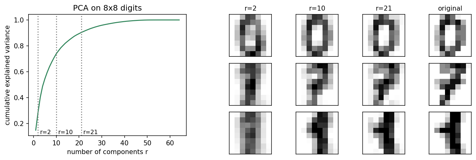
Twenty-one of the 64 pixel dimensions hold 90% of the variance of the digits, and the reconstruction from them has a relative error of 0.31. The hand-written SVD agrees with scikit-learn up to the sign of each component (an eigenvector’s sign is arbitrary). Figure 1 shows the cumulative curve and reconstructions.
Variance is not class information
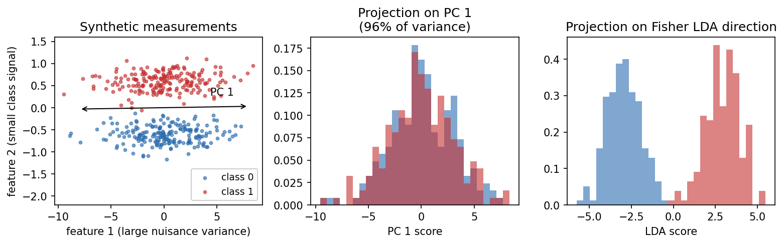
PCA ranks directions by variance, and variance is not the same as usefulness for classification. In Figure 2, a large nuisance variation (think lighting) dominates the first principal component, while the class difference lives in a direction with small variance. Projecting onto PC 1 keeps 96% of the variance and throws away essentially all the class information. A supervised projection (Fisher’s LDA, next section) finds the useful direction immediately.
Jolliffe and Cadima’s review [10] covers what PCA can and cannot do, and its many variants (for example sparse and robust PCA). Probabilistic PCA and factor analysis, which turn PCA into a latent-variable model, are developed in Bishop, Chapter 12 [2], and in ML 06A.
Fisher’s linear discriminant analysis
In plain words. LDA looks for the directions in which the class means are far apart relative to how spread out each class is. It uses the labels, so it finds directions that matter for classification, but it can produce at most one fewer direction than there are classes.
Fisher’s criterion for a projection direction is the ratio of between-class to within-class scatter along [11]:
with and as defined in the previous section. Setting the gradient to zero gives the generalized eigenproblem
and the best directions are the eigenvectors with the largest eigenvalues (equivalently, eigenvectors of when is invertible) [1], [2]. For two classes there is a closed form, , which reappears as the Gaussian LDA classifier in PR 03.
Why at most directions. is a weighted sum of rank-one matrices . The vectors are linearly dependent, because . So has rank at most , and at most eigenvalues are nonzero. Ten digit classes give at most nine discriminant directions, whatever the input dimension.
When is singular. With fewer samples than features (common with images), cannot be inverted. Standard fixes are to apply PCA first and then LDA in the reduced space, or to shrink toward a multiple of the identity (regularized LDA).
Code · Python · 17 lines
from sklearn.datasets import load_digits
from sklearn.discriminant_analysis import LinearDiscriminantAnalysis as LDA
from sklearn.model_selection import cross_val_score
from sklearn.neighbors import KNeighborsClassifier
from sklearn.pipeline import make_pipeline
from sklearn.decomposition import PCA
from sklearn.preprocessing import StandardScaler

X, y = load_digits(return_X_y=True)
lda = LDA().fit(X, y)
print("discriminant directions for 10 classes:", lda.transform(X).shape[1])
for name, reducer in [("PCA", PCA(n_components=2)),
                      ("LDA", LDA(n_components=2))]:
    pipe = make_pipeline(StandardScaler(), reducer,
                         KNeighborsClassifier(n_neighbors=5))
    acc = cross_val_score(pipe, X, y, cv=5).mean()
    print(f"{name} to 2-D, then 5-NN: CV accuracy {acc:.3f}")
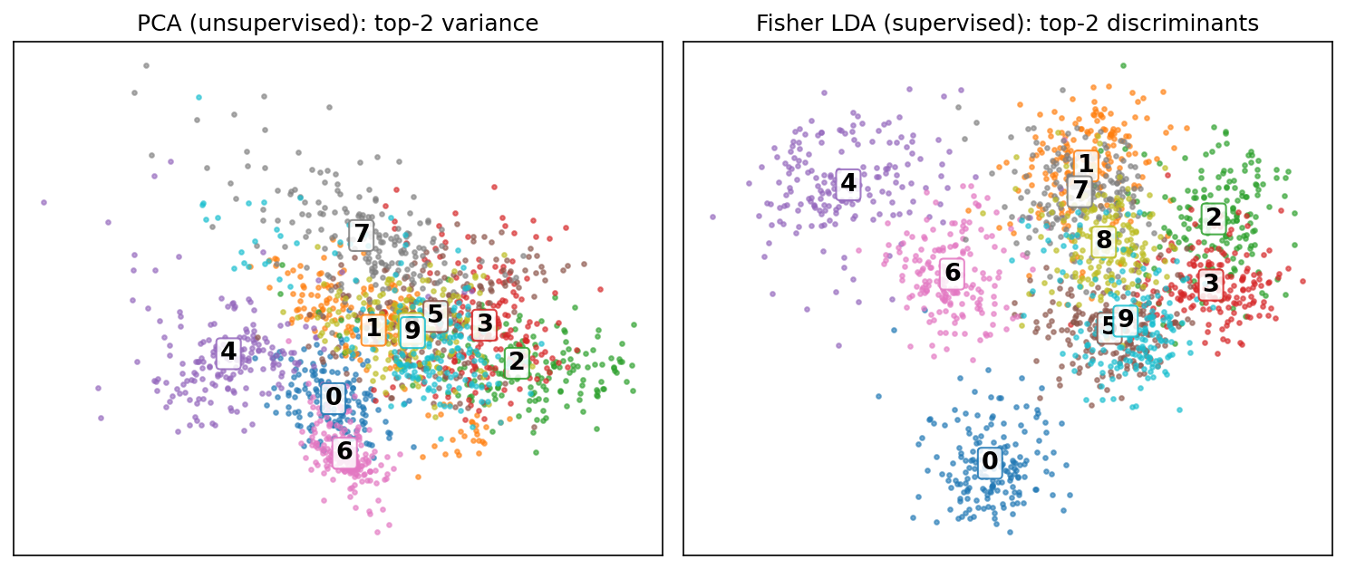
LDA returns nine directions for ten classes, as predicted. Squeezed to two dimensions, a 5-NN classifier on LDA coordinates reaches a cross-validated accuracy of 0.624, against 0.512 on the first two principal components. Because LDA uses labels, it sits inside the pipeline and is refitted in every fold. Figure 3 shows why: LDA pulls whole digit classes apart, while PCA mostly shows the directions of largest pixel variation.
Kernel PCA
In plain words. Kernel PCA is PCA performed in the rich feature space of a kernel (PR 04), without ever computing the features. It can unroll structures that no linear projection can.
Schölkopf, Smola and Müller showed that PCA in the feature space only needs the kernel matrix [12]. Center it in feature space,
where is the matrix with every entry . Solve the eigenproblem for coefficient vectors , normalized so that . The -th kernel principal component of a point is then
where is the kernel centered in the same way. The cost is that of an eigenproblem, and a new point needs kernel evaluations.
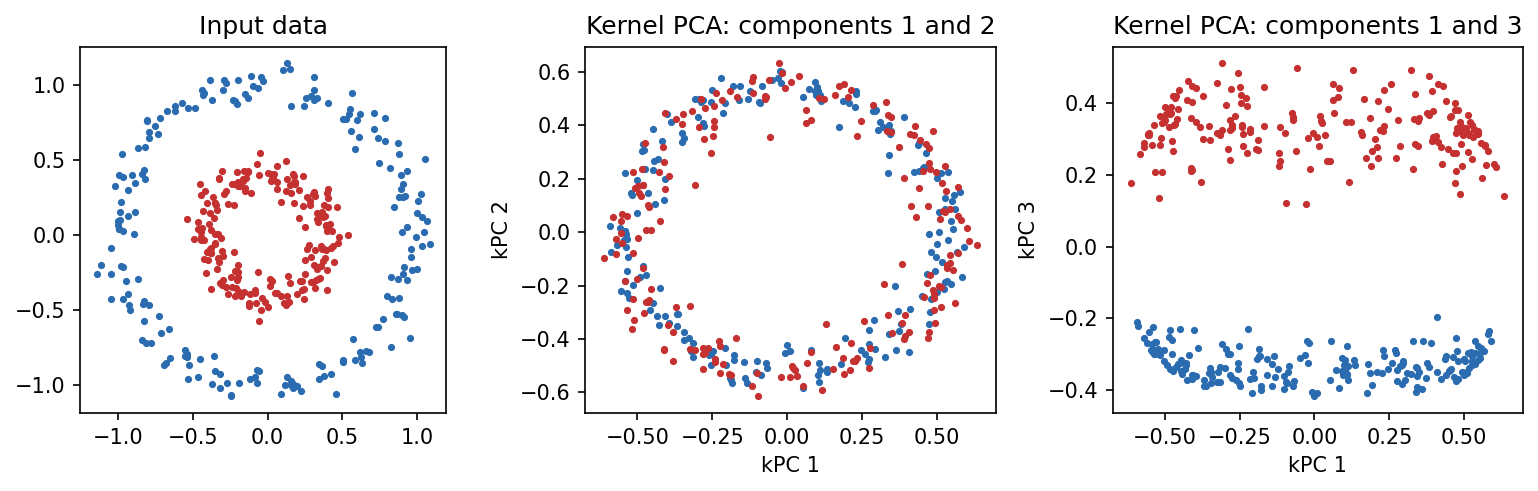
Kernel PCA is still unsupervised: it ranks components by variance in feature space, not by class separation. On the two-ring data, the first two RBF kernel components describe the angle around the rings and mix the classes; the third component describes the radius and separates them perfectly (Figure 4).
Code · Python · 18 lines
import numpy as np
from sklearn.datasets import make_circles
from sklearn.decomposition import PCA, KernelPCA
from sklearn.linear_model import LogisticRegression
from sklearn.model_selection import cross_val_score
from sklearn.pipeline import make_pipeline

X, y = make_circles(n_samples=400, factor=0.4, noise=0.07, random_state=0)
Z = KernelPCA(n_components=4, kernel="rbf", gamma=2).fit_transform(X)
print("|corr(component, label)|:",
      np.round([abs(np.corrcoef(Z[:, i], y)[0, 1]) for i in range(4)], 3))

for name, reducer in [("linear PCA, 2 comps", PCA(n_components=2)),
                      ("kernel PCA, 3 comps", KernelPCA(n_components=3,
                                                        kernel="rbf", gamma=2))]:
    acc = cross_val_score(make_pipeline(reducer, LogisticRegression()),
                          X, y, cv=5).mean()
    print(f"{name} -> logistic regression: {acc:.3f}")
Only the third component correlates with the label (0.982; the others are below 0.05). A logistic regression on the two linear principal components cannot beat chance (0.432), while on three kernel components it is perfect (1.000).
Independent component analysis
In plain words. At a party, two microphones each record a mixture of two voices. ICA tries to recover the individual voices from the mixtures alone, using the fact that the voices are statistically independent and not Gaussian.
ICA assumes the observed vector is a linear mixture of independent sources [13]:
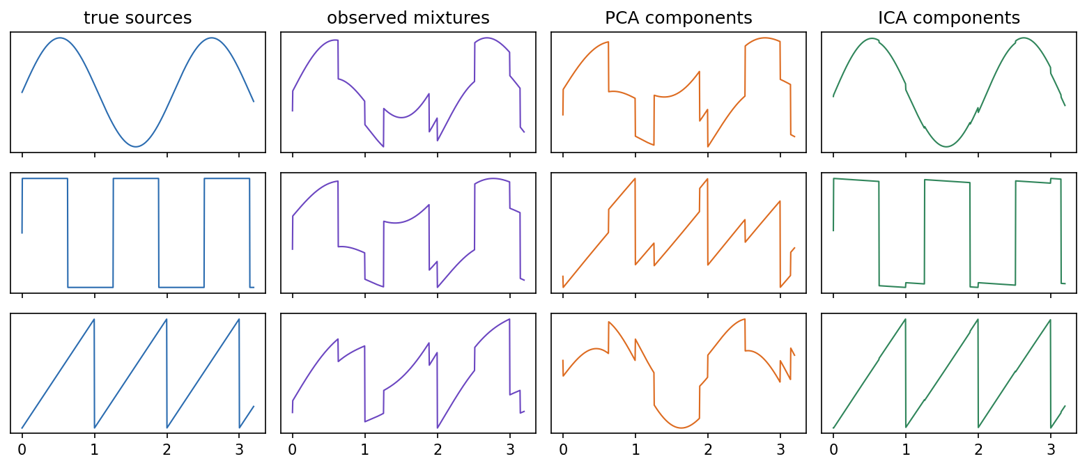
where are statistically independent, non-Gaussian source signals, is an unknown mixing matrix and are the observed signals. The goal is an unmixing matrix such that has independent components. Why non-Gaussian? By the central limit theorem, mixtures tend to be “more Gaussian” than their sources, so maximizing the non-Gaussianity of finds a source. FastICA measures non-Gaussianity with approximations of negentropy and runs a fixed-point iteration after whitening the data [13]. Two ambiguities can never be resolved: the order of the sources and their scale (including sign).
The contrast with PCA is the point. PCA only makes the components uncorrelated (second-order statistics); ICA makes them independent, using higher-order statistics. If the sources were Gaussian, uncorrelated would already mean independent, and any rotation of the whitened data would be equally good, so ICA would fail.
Code · Python · 16 lines
import numpy as np
from sklearn.decomposition import FastICA

t = np.linspace(0, 8, 2000)
S = np.c_[np.sin(3 * t),                      # source 1: sine
          np.sign(np.sin(5 * t)),             # source 2: square wave
          ((2 * t) % 2) - 1]                  # source 3: sawtooth
A = np.array([[1.0, 0.5, 0.3],
              [0.6, 1.0, 0.4],
              [0.4, 0.3, 1.0]])               # unknown mixing matrix
X = S @ A.T                                   # what the sensors record

S_hat = FastICA(n_components=3, whiten="unit-variance",
                random_state=0).fit_transform(X)
corr = np.abs(np.corrcoef(S.T, S_hat.T)[:3, 3:])
print(np.round(corr, 3))                      # one entry near 1 per row
Each true source matches exactly one recovered component with absolute correlation 0.999 or 1.000, and the off-diagonal matches are below 0.05. Figure 5 shows that PCA, applied to the same mixtures, returns uncorrelated signals that are still mixtures.
Non-negative matrix factorization (NMF) is a related decomposition for non-negative data such as pixel intensities or word counts: it writes with elementwise. Because nothing can be subtracted, the factors tend to be additive “parts,” as Lee and Seung showed for face images [14].
Manifold learning
In plain words. Sometimes high-dimensional data lie on a curved, low-dimensional sheet, like a rolled-up poster. Manifold learning tries to unroll the sheet, keeping points that were neighbors along the sheet close together, without being fooled by points that are close in 3-D only because the sheet is rolled up.
The Swiss roll in Figure 6 is the standard example: a two-dimensional rectangle rolled up in three dimensions. PCA flattens it by projection and puts different layers of the roll on top of each other. Neighborhood-based methods do better:
- Isomap [15] builds a -nearest-neighbor graph, estimates geodesic distances along the manifold as shortest-path lengths in the graph, and then finds low-dimensional coordinates whose Euclidean distances match those geodesic distances (classical multidimensional scaling).
- Locally linear embedding (LLE) [16] writes each point as a weighted combination of its neighbors, with , and then finds low-dimensional points that are reconstructed by the same weights.
- t-SNE [17] converts distances into neighbor probabilities in the input (Gaussian, with a bandwidth set by a “perplexity” parameter) and in the embedding (heavy-tailed Student-), and minimizes the Kullback–Leibler divergence . The heavy tails let well-separated groups spread out.
- UMAP [18] builds a weighted -nearest-neighbor graph (a “fuzzy” topological representation) and optimizes a low-dimensional layout with a cross-entropy objective. It is typically faster than t-SNE and is often used for the same purpose.
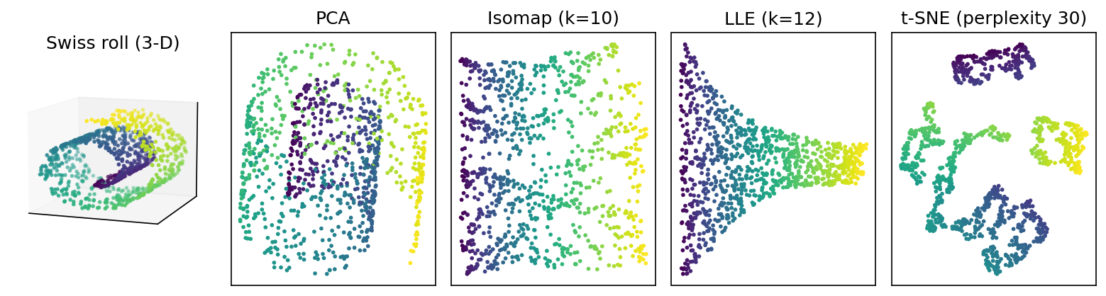
One quantitative check is trustworthiness: the extent to which the nearest neighbors of each point in the embedding were also near neighbors in the input (1.0 is perfect).
Code · Python · 17 lines
from sklearn.datasets import make_swiss_roll
from sklearn.decomposition import PCA
from sklearn.manifold import Isomap, LocallyLinearEmbedding, TSNE, trustworthiness

X, t = make_swiss_roll(n_samples=1000, noise=0.05, random_state=0)
methods = {
    "PCA": PCA(n_components=2),
    "Isomap": Isomap(n_neighbors=10, n_components=2),
    "LLE": LocallyLinearEmbedding(n_neighbors=12, n_components=2,
                                  random_state=0),
    "t-SNE": TSNE(n_components=2, perplexity=30, init="pca",
                  random_state=0),
}
for name, method in methods.items():
    Y = method.fit_transform(X)
    print(f"{name:7s} trustworthiness (k=10): "
          f"{trustworthiness(X, Y, n_neighbors=10):.3f}")
PCA scores 0.905; Isomap and t-SNE 0.999; LLE 0.996. Note what the number does not see: t-SNE scores as high as Isomap even though Figure 6 shows it tearing the roll into islands. Local neighborhoods are preserved; global structure is not.
What an embedding picture can and cannot prove
These methods are mainly tools for looking at data. Three cautions follow from how they work [19]:
- Cluster sizes and gaps are not meaningful by default. t-SNE normalizes local densities, so a tight cluster and a diffuse one can look the same size, and distances between clusters may say little.
- Results depend on settings. Perplexity, number of neighbors, initialization and random seed all change the picture. Wattenberg, Viégas and Johnson’s interactive article shows the same data producing very different t-SNE maps [19].
- Two dimensions may not be enough. A projection to 2-D must distort high-dimensional distances; well-separated islands in a picture are not proof of separate populations.
There is also a practical gap for classification: t-SNE and standard LLE learn coordinates for the training points only, with no natural rule for embedding a new point. Isomap, kernel PCA and UMAP provide out-of-sample transforms, but if a nonlinear embedding is part of a classifier, it must be fitted inside the training folds like any other step.
Image and signal descriptors
In plain words. Before features were learned, people designed them by hand to measure exactly the properties they believed mattered: texture, edges, shape, frequency content. They remain useful as baselines and as interpretable checks.
Theodoridis and Koutroumbas devote two chapters to transform-based and application-specific features [1]; IP 12 treats image descriptors in detail. Consider what each one keeps and what it is sensitive to:
| Descriptor | Preserves | Typical sensitivity |
|---|---|---|
| Intensity histogram | Distribution of values | Loses spatial arrangement entirely |
| Co-occurrence (GLCM) statistics [20] | Pairwise intensity relations at an offset | Quantization levels and offset direction |
| Histogram of oriented gradients (HOG) [21] | Local edge directions in a grid of cells | Cropping, scale and alignment |
| Area, perimeter, compactness | Region geometry | Segmentation errors and resolution |
| Fourier/DCT coefficients | Frequency content | Alignment and which frequencies are kept |
| Wavelet coefficients | Location and scale of variation | Basis choice and boundary handling |
For a quantized image and an offset , a gray-level co-occurrence matrix counts pairs over pixel positions ; normalized to probabilities , Haralick’s texture features include contrast and energy [20]. Always state the offset and the number of gray levels, because the numbers depend on both. For a segmented object with area and perimeter , compactness equals 1 for an ideal continuous circle and is smaller for irregular shapes; pixel-based perimeter estimates distort it for small objects. Dalal and Triggs’ HOG descriptor, built from normalized histograms of gradient orientation in small cells, was introduced for pedestrian detection and became one of the most widely used hand-designed image features [21].
For audio and other 1-D signals, features are computed on short windows in which the signal is approximately stationary: spectral energy in frequency bands, zero-crossing rate, and so on. The window length trades time resolution against frequency resolution.
Code: one classifier, three feature sets
This example compares fixed feature strategies with the same classifier on the built-in digits data.
Code · Python · 21 lines
from sklearn.datasets import load_digits
from sklearn.model_selection import train_test_split
from sklearn.pipeline import make_pipeline
from sklearn.preprocessing import StandardScaler
from sklearn.decomposition import PCA
from sklearn.feature_selection import SelectKBest, f_classif
from sklearn.linear_model import LogisticRegression

X, y = load_digits(return_X_y=True)
Xtr, Xte, ytr, yte = train_test_split(
    X, y, test_size=0.25, stratify=y, random_state=9)
transforms = {
    "all features": "passthrough",
    "24 PCA coordinates": PCA(n_components=24, random_state=9),
    "24 selected coordinates": SelectKBest(f_classif, k=24),
}
for name, transform in transforms.items():
    model = make_pipeline(
        StandardScaler(), transform, LogisticRegression(max_iter=1500))
    model.fit(Xtr, ytr)
    print(name, "test accuracy:", round(model.score(Xte, yte), 4))
All 64 pixels give 0.969 test accuracy, 24 principal components 0.956, and the 24 pixels with the best ANOVA scores 0.953. Here a reduction to about a third of the dimensions costs little accuracy. Some border pixels of the digits are constant, so the test warns about constant features; the warning reflects zero within-class variance, not leakage, and those pixels simply receive no useful score.
Modern view
Feature engineering by hand has largely given way to learned representations, but the ideas of this chapter are everywhere in modern pipelines: deep features are selected, projected, whitened, visualized and evaluated with the same tools. Here is how the survey literature maps the field.
Feature selection. Guyon and Elisseeff’s introduction [3] set the vocabulary (filters, wrappers, embedded methods), discussed feature construction, ranking and validation, and stressed that a feature can be useless alone and useful in combination. Chandrashekar and Sahin [23] provide a compact survey organized along the same filter/wrapper/embedded lines. Li et al. [22] revisit selection “from a data perspective”: they group algorithms for conventional data into similarity-based, information-theoretic, sparse-learning-based and statistical methods, add methods for structured, heterogeneous and streaming data, and release an open-source repository for benchmarking. The leakage warning of Ambroise and McLachlan [7] remains the single most important practical lesson.
PCA and its descendants. Jolliffe and Cadima’s review [10] explains PCA as an adaptive, data-defined technique and surveys its variants tailored to different data types. In modern deep learning, PCA survives as a diagnostic (how many directions carry most variance in a layer’s activations) and as a preprocessing and initialization step, for example the PCA initialization recommended for t-SNE [26].
Dimensionality reduction for visualization. Espadoto et al. [24] ran a large quantitative survey of projection techniques: they characterized data sets, techniques and projection quality with several quantitative metrics (such as neighborhood and distance preservation), measured how the results depend on the technique and the data, and turned the observations into guidance for choosing a projection in a given context, with all code and results released as an open benchmark. Wang, Huang, Rudin and Shaposhnik [25] analyzed why t-SNE, UMAP and TriMAP behave as they do, focused on the trade-off between preserving local and global structure, and proposed PaCMAP to balance the two.
Pitfalls of 2-D embeddings. Single-cell biology, where t-SNE and UMAP are routine, produced the sharpest critiques. Kobak and Berens [26] gave a protocol for more faithful t-SNE maps: PCA initialization, a high learning rate and multi-scale similarities. Kobak and Linderman [27] showed that the better global structure often credited to UMAP comes largely from its initialization; with the same informative initialization, t-SNE preserves global structure similarly. Chari and Pachter [28] went further, arguing that extreme reduction to two dimensions inevitably distorts high-dimensional data and that such pictures should not be used for quantitative conclusions.
Variance versus usefulness, revisited. Figure 2’s lesson reappears at scale in self-supervised learning. Balestriero and LeCun [29] argue that training a representation to reconstruct its input emphasizes high-variance components of the data, which are often less informative for perception tasks than low-variance details; reconstruction-trained features therefore need extra steps (such as fine-tuning) to be useful for classification. This is PCA’s limitation, in a deep-learning setting.
Open problems. Selection with many correlated features and few samples remains unstable: different subsets can perform equally well, which complicates interpretation. Evaluating embeddings still lacks agreed metrics that capture both local and global fidelity [24], [25]. And for learned features, deciding which directions carry task-relevant rather than merely high-variance information is an active research question [29].
Key takeaways
- Feature selection keeps original measurements; extraction builds new coordinates; learning fits the extraction rule from data. All three decide what the classifier can see.
- Filters are fast but miss interactions and redundancy; wrappers see them but cost more and can overfit validation data; embedded methods (lasso, trees) select during training.
- Any step that uses labels (selection, LDA, choosing the number of features) must be refitted inside each cross-validation fold. Selecting on the full data can report 98% accuracy on pure noise.
- Fisher ratio, , Bhattacharyya distance and mutual information score features; subsets must be scored jointly because of redundancy.
- PCA keeps maximum variance (eigenvectors of the covariance, computed by SVD); whitening equalizes variances. Variance is not class information.
- Fisher LDA solves and gives at most directions. Kernel PCA, ICA and NMF extend linear extraction to nonlinear, independent or non-negative structure.
- Isomap, LLE, t-SNE and UMAP are mainly visualization tools: their pictures depend on settings, and gaps between clusters are not proof of separate populations.
Exercises
- Same histogram, different image. Construct two binary images with identical intensity histograms but different texture. Which descriptor from the table distinguishes them?
Hint
Use eight 1-pixels arranged as a checkerboard versus the left half filled. The histograms are identical. A co-occurrence matrix with horizontal offset distinguishes them: the checkerboard has only unequal neighbor pairs, the half-filled image mostly equal ones.
- The limit. Prove that the between-class scatter of classes has rank at most . What does this imply for LDA on a two-class problem?
Hint
with , and , so the vectors span at most dimensions. With two classes, LDA gives a single direction, .
- When 99% of the variance is not enough. Describe a realistic imaging setup in which keeping 99% of the PCA variance discards the class signal. How would you detect the problem, and what would you do?
Hint
Large independent lighting or pose changes plus a small, consistent defect mark (Figure 2 in disguise). Detect it by comparing cross-validated accuracy with and without PCA, or by checking class separation (Fisher ratio) per component. Use a supervised projection, normalize the nuisance (for example illumination) first, or skip PCA.
- The XOR trap. Generate uniform on and eight irrelevant noise features, with . Rank all ten features with
f_classifand withmutual_info_classif. Then run sequential forward selection with a decision tree. Which methods find and ?
Hint
Both univariate filters give and scores near zero, like the noise features, because each alone is independent of . A wrapper that adds features one at a time can also struggle at the first step, for the same reason; a tree-based wrapper that evaluates pairs, or backward elimination starting from all features, finds them.
- Leakage, quantified. In the selection-bias code, vary the number of noise features (100, 1,000, 5,000) and the number of samples (30, 60, 200). How does the “wrong” accuracy change? Explain the trend.
Hint
The optimism grows with the number of candidate features and shrinks with the number of samples: with more noise features, more of them correlate with the labels by chance in a small sample, and selecting the best 20 picks exactly those.
- Reading a t-SNE map. Run t-SNE on the digits data with perplexity 5, 30 and 100, and with two random seeds each. Which features of the plots are stable (which digits are neighbors?) and which change (cluster sizes, gaps, positions)? What would you be willing to claim from one such plot?
Hint
Membership of local neighborhoods is quite stable; absolute positions, cluster areas and between-cluster distances are not. A defensible claim is “these points are locally similar in the input space,” not “these two groups are far apart” or “this group is twice as diverse.”
References
- S. Theodoridis and K. Koutroumbas, Pattern Recognition, 4th ed., Academic Press, 2009, Chapters 5–7. publisher page
- C. M. Bishop, Pattern Recognition and Machine Learning, Springer, 2006, Sections 4.1.4–4.1.6 and 12.1–12.4. official book page and PDF
- I. Guyon and A. Elisseeff, “An Introduction to Variable and Feature Selection,” Journal of Machine Learning Research, vol. 3, pp. 1157–1182, 2003. JMLR
- R. Kohavi and G. H. John, “Wrappers for Feature Subset Selection,” Artificial Intelligence, vol. 97, pp. 273–324, 1997. doi:10.1016/S0004-3702(97)00043-X
- R. Tibshirani, “Regression Shrinkage and Selection via the Lasso,” Journal of the Royal Statistical Society, Series B, vol. 58, no. 1, pp. 267–288, 1996. doi:10.1111/j.2517-6161.1996.tb02080.x
- H. Peng, F. Long, and C. Ding, “Feature Selection Based on Mutual Information: Criteria of Max-Dependency, Max-Relevance, and Min-Redundancy,” IEEE Transactions on Pattern Analysis and Machine Intelligence, vol. 27, no. 8, pp. 1226–1238, 2005. doi:10.1109/TPAMI.2005.159
- C. Ambroise and G. J. McLachlan, “Selection Bias in Gene Extraction on the Basis of Microarray Gene-Expression Data,” Proceedings of the National Academy of Sciences, vol. 99, no. 10, pp. 6562–6566, 2002. doi:10.1073/pnas.102102699
- K. Pearson, “On Lines and Planes of Closest Fit to Systems of Points in Space,” The London, Edinburgh, and Dublin Philosophical Magazine and Journal of Science, vol. 2, no. 11, pp. 559–572, 1901. doi:10.1080/14786440109462720
- H. Hotelling, “Analysis of a Complex of Statistical Variables into Principal Components,” Journal of Educational Psychology, vol. 24, no. 6, pp. 417–441, 1933. doi:10.1037/h0071325
- I. T. Jolliffe and J. Cadima, “Principal Component Analysis: A Review and Recent Developments,” Philosophical Transactions of the Royal Society A, vol. 374, 20150202, 2016. doi:10.1098/rsta.2015.0202
- R. A. Fisher, “The Use of Multiple Measurements in Taxonomic Problems,” Annals of Eugenics, vol. 7, no. 2, pp. 179–188, 1936. doi:10.1111/j.1469-1809.1936.tb02137.x
- B. Schölkopf, A. Smola, and K.-R. Müller, “Nonlinear Component Analysis as a Kernel Eigenvalue Problem,” Neural Computation, vol. 10, no. 5, pp. 1299–1319, 1998. doi:10.1162/089976698300017467
- A. Hyvärinen and E. Oja, “Independent Component Analysis: Algorithms and Applications,” Neural Networks, vol. 13, no. 4–5, pp. 411–430, 2000. doi:10.1016/S0893-6080(00)00026-5
- D. D. Lee and H. S. Seung, “Learning the Parts of Objects by Non-Negative Matrix Factorization,” Nature, vol. 401, pp. 788–791, 1999. doi:10.1038/44565
- J. B. Tenenbaum, V. de Silva, and J. C. Langford, “A Global Geometric Framework for Nonlinear Dimensionality Reduction,” Science, vol. 290, no. 5500, pp. 2319–2323, 2000. doi:10.1126/science.290.5500.2319
- S. T. Roweis and L. K. Saul, “Nonlinear Dimensionality Reduction by Locally Linear Embedding,” Science, vol. 290, no. 5500, pp. 2323–2326, 2000. doi:10.1126/science.290.5500.2323
- L. van der Maaten and G. Hinton, “Visualizing Data using t-SNE,” Journal of Machine Learning Research, vol. 9, pp. 2579–2605, 2008. JMLR
- L. McInnes, J. Healy, and J. Melville, “UMAP: Uniform Manifold Approximation and Projection for Dimension Reduction,” arXiv:1802.03426, 2018. arXiv
- M. Wattenberg, F. Viégas, and I. Johnson, “How to Use t-SNE Effectively,” Distill, 2016. doi:10.23915/distill.00002
- R. M. Haralick, K. Shanmugam, and I. Dinstein, “Textural Features for Image Classification,” IEEE Transactions on Systems, Man, and Cybernetics, vol. SMC-3, no. 6, pp. 610–621, 1973. doi:10.1109/TSMC.1973.4309314
- N. Dalal and B. Triggs, “Histograms of Oriented Gradients for Human Detection,” IEEE Conference on Computer Vision and Pattern Recognition (CVPR), vol. 1, pp. 886–893, 2005. doi:10.1109/CVPR.2005.177
- J. Li, K. Cheng, S. Wang, F. Morstatter, R. P. Trevino, J. Tang, and H. Liu, “Feature Selection: A Data Perspective,” ACM Computing Surveys, vol. 50, no. 6, 2018. doi:10.1145/3136625
- G. Chandrashekar and F. Sahin, “A Survey on Feature Selection Methods,” Computers & Electrical Engineering, vol. 40, no. 1, pp. 16–28, 2014. doi:10.1016/j.compeleceng.2013.11.024
- M. Espadoto, R. M. Martins, A. Kerren, N. S. T. Hirata, and A. C. Telea, “Toward a Quantitative Survey of Dimension Reduction Techniques,” IEEE Transactions on Visualization and Computer Graphics, vol. 27, no. 3, pp. 2153–2173, 2021. doi:10.1109/TVCG.2019.2944182
- Y. Wang, H. Huang, C. Rudin, and Y. Shaposhnik, “Understanding How Dimension Reduction Tools Work: An Empirical Approach to Deciphering t-SNE, UMAP, TriMAP, and PaCMAP for Data Visualization,” Journal of Machine Learning Research, vol. 22, 2021. arXiv:2012.04456
- D. Kobak and P. Berens, “The Art of Using t-SNE for Single-Cell Transcriptomics,” Nature Communications, vol. 10, 2019. doi:10.1038/s41467-019-13056-x
- D. Kobak and G. C. Linderman, “Initialization Is Critical for Preserving Global Data Structure in Both t-SNE and UMAP,” Nature Biotechnology, vol. 39, pp. 156–157, 2021. doi:10.1038/s41587-020-00809-z
- T. Chari and L. Pachter, “The Specious Art of Single-Cell Genomics,” PLOS Computational Biology, vol. 19, e1011288, 2023. doi:10.1371/journal.pcbi.1011288
- R. Balestriero and Y. LeCun, “Learning by Reconstruction Produces Uninformative Features for Perception,” arXiv:2402.11337, 2024. arXiv
Check your understanding
This tutorial has 6 exercises. Can you solve them without opening the hints?
Go to the exercises ↑Next PR 06 · Template Matching and Structured Recognition · 24 min