PR 02 · Density Estimation and Bayesian Learning
Needs: PR 01 · Patterns, Probability and Bayes Decisions, ML 01A · Linear Algebra for Learning
Navigate: this page and this track: Navigate: this page and this track
On this page
- What you’ll learn1 min
- The big picture2 min
- Maximum-likelihood estimation2 min
- MAP and Bayesian estimation3 min
- Classifiers built from densities1 min
- Non-parametric estimation: one formula, three estimators5 min
- The kkk-nearest-neighbor classifier2 min
- The curse of dimensionality2 min
- Modern view2 min
- Key takeaways1 min
- Exercises2 min
- References
Pattern Recognition
Explore this chapter 1 interactive experiment
Change the bandwidth and inspect individual kernels, the estimated density and leave-one-out prediction.
What you’ll learn
- Why a Bayes classifier needs density estimates, and the difference between parametric and non-parametric estimation.
- How to derive maximum-likelihood (ML) estimates for a Gaussian, why the covariance becomes singular with few samples, and how shrinkage fixes it.
- How MAP and full Bayesian estimation use a prior over parameters, worked out for a Gaussian mean and a Bernoulli rate.
- How histograms, Parzen windows (kernel density estimation) and -nearest-neighbor estimates follow from one formula, and how to choose the bandwidth or .
- How the -NN classifier falls out of -NN density estimation, what the Cover–Hart bound says, and why all local methods suffer from the curse of dimensionality.
The big picture
PR 01 showed that the best possible classifier needs the class priors and the class-conditional densities . In practice nobody hands us these distributions; we have a finite set of labelled examples. This chapter is about turning examples into densities. Once we have and , we can plug them into the Bayes rule. This is the generative route to classification. The next chapter takes the discriminative route and fits the decision boundary directly.
There are two families of estimators [1, 2, 3]:
- Parametric methods assume a functional form, such as a Gaussian, and estimate a fixed number of parameters. They need little data when the form is right and give systematically wrong answers when it is wrong.
- Non-parametric methods let the data decide the shape. Their complexity grows with the number of samples. They are flexible but need much more data, especially in high dimensions.
Both families face the same central question: how much structure can the available data support? A flexible estimator can describe the training data beautifully and still predict new data poorly. Every method below has a “smoothness knob” (the number of parameters, the prior, the bin width, the bandwidth, ), and choosing it well matters more than choosing the method.
Maximum-likelihood estimation
Plain version. Choose the parameter values under which the observed data would have been most probable.
Precise version. Let be samples drawn independently from a density with unknown parameter vector . The likelihood of is , and the ML estimate maximizes its logarithm:
The independence assumption is about sampling (different observations do not influence each other), not about independence between the coordinates of one feature vector. For a classifier we fit one model per class, using only that class’s samples, and estimate the prior as the class frequency .
The Gaussian case
For a -dimensional Gaussian the log-likelihood is
Setting the gradient with respect to to zero gives . Differentiating with respect to (using and ) gives the estimates
The sample mean is unbiased. The ML covariance is slightly biased: , because was fitted to the same data and sits closer to them than the true mean does. The familiar sample covariance divides by to remove this bias. For large the difference is negligible.
When ML breaks: too many parameters
A full covariance has distinct entries. With features that is numbers per class, plus for the mean. Worse, is a sum of rank-one matrices centered at , so its rank is at most . When a class has no more samples than dimensions, its ML covariance is singular: it has zero variance in some directions, , and the Gaussian discriminant of PR 01 is undefined. Even when is a bit larger than , the smallest eigenvalues are systematically underestimated, and the inverse hugely amplifies noise along those directions.
Regularization shrinks the covariance towards a simpler target:
Here is a spherical matrix with the same average variance, and is the shrinkage intensity. Shrinkage pulls large eigenvalues down and small ones up, trading a little bias for a much better-conditioned estimate. Ledoit and Wolf [14] derived a closed-form estimate of the that minimizes the expected squared error, so it needs no cross-validation. Other common restrictions are a diagonal covariance (ignore correlations; this is Gaussian naive Bayes, below) and a shared covariance across classes (pool the evidence; this is LDA from PR 01). These are different modelling assumptions, not interchangeable numerical tricks.
Code: when the ML covariance fails
Code · Python · 21 lines
import numpy as np
from scipy.stats import multivariate_normal
from sklearn.covariance import EmpiricalCovariance, LedoitWolf

rng = np.random.default_rng(0)
d = 40
A = rng.normal(size=(d, d))
true_cov = A @ A.T / d + 0.5 * np.eye(d)          # a well-conditioned truth
test = rng.multivariate_normal(np.zeros(d), true_cov, 2000)

for n in [30, 60, 200, 1000]:
    train = rng.multivariate_normal(np.zeros(d), true_cov, n)
    mu = train.mean(0)
    S_ml = EmpiricalCovariance().fit(train).covariance_   # divisor n
    S_lw = LedoitWolf().fit(train)
    rank = np.linalg.matrix_rank(S_ml)
    ll_ml = (multivariate_normal(mu, S_ml, allow_singular=True).logpdf(test).mean()
             if rank == d else -np.inf)
    ll_lw = multivariate_normal(mu, S_lw.covariance_).logpdf(test).mean()
    print(f"n={n:4d}: rank(S_ML)={rank:2d}, test log-lik ML={ll_ml:8.2f}, "
          f"Ledoit-Wolf={ll_lw:8.2f} (shrinkage {S_lw.shrinkage_:.2f})")
With and the ML covariance has rank and assigns zero density to almost every test point (log-likelihood ). At it is invertible but poor (test log-likelihood versus for Ledoit–Wolf). The automatically chosen shrinkage falls from to as grows, and at the two estimates almost coincide. The rule of thumb: the fewer samples per parameter, the more you should shrink.
MAP and Bayesian estimation
Plain version. Maximum likelihood trusts the data completely. Bayesian estimation starts from a prior belief about the parameters and lets the data gradually overrule it. With little data the prior matters; with lots of data it hardly does.
Precise version. Treat as a random variable with a parameter prior . Bayes’ rule gives the parameter posterior
A parameter prior is different from the class prior of PR 01. The class prior says how common a category is; a parameter prior says which model settings are plausible before seeing this training set. Three ways to use the posterior are common:
- MAP estimation keeps only its mode: . The log prior acts as a regularizer; a Gaussian prior on weights is exactly an (ridge) penalty, which PR 03 uses.
- Full Bayesian prediction averages over all parameter values instead of choosing one:
This posterior predictive distribution carries parameter uncertainty into the prediction.
- Plug-in prediction uses with from ML or MAP. It ignores parameter uncertainty and is therefore overconfident when data are scarce.
One subtle point: MAP is not invariant to re-parameterization. The mode of a density over is not the square root of the mode of the corresponding density over , because densities pick up a Jacobian factor when the variable changes. ML estimates and full posteriors do not have this problem.
Worked example: the mean of a Gaussian
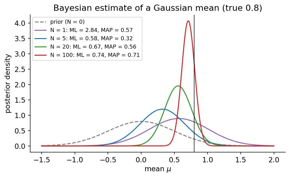
Let with known , and put a Gaussian prior on the unknown mean, . Multiplying the likelihood and the prior and completing the square in shows that the posterior is again Gaussian, , with [1, 2]
where is the sample mean. Two readings make this formula memorable. Precisions add: the posterior precision is the prior precision plus times the precision of one observation. The mean is a precision-weighted average of the prior mean and the sample mean. As , (the ML estimate) and . Since the posterior is Gaussian, its mode equals its mean, so here . The posterior predictive is : wider than the plug-in by the remaining uncertainty about .
A prior whose posterior stays in the same family is called conjugate. Conjugate pairs (Gaussian–Gaussian, Beta–Bernoulli, Dirichlet–categorical, Normal–inverse-Wishart for a mean and covariance) give closed-form updates; other priors require the approximate inference methods of PR 08.
Worked example: a Bernoulli rate
For a Bernoulli rate (for instance the defect rate on a line) with prior , observing successes in trials gives
The prior acts like imaginary successes and imaginary failures. With one success and no failures, ML predicts probability one, which is absurd. A uniform prior predicts ; this is Laplace’s rule of succession. The same idea, called additive or Laplace smoothing, keeps a naive Bayes text classifier from assigning zero probability to a document because one word never appeared with a class in training.
Code: ML, MAP and the posterior predictive
Code · Python · 22 lines
import numpy as np

rng = np.random.default_rng(3)
sigma = 1.0                 # known noise standard deviation
m0, s0 = 0.0, 0.5           # prior on the mean: N(m0, s0^2)
x = rng.normal(0.8, sigma, 5)
n = len(x)

mu_ml = x.mean()
post_var = 1 / (1 / s0**2 + n / sigma**2)
post_mean = post_var * (m0 / s0**2 + x.sum() / sigma**2)   # = MAP for a Gaussian
pred_var = sigma**2 + post_var                              # predictive variance

# brute-force check on a grid: posterior is proportional to likelihood x prior
grid = np.linspace(-3, 3, 200001)
log_post = (-0.5 * ((x[:, None] - grid) ** 2).sum(0) / sigma**2
            - 0.5 * (grid - m0) ** 2 / s0**2)
w = np.exp(log_post - log_post.max())
w /= w.sum()
print(f"ML {mu_ml:.3f} | MAP/posterior mean {post_mean:.3f} "
      f"(grid {np.sum(w * grid):.3f}) | posterior sd {np.sqrt(post_var):.3f}")
print(f"predictive sd {np.sqrt(pred_var):.3f} vs plug-in sd {sigma:.3f}")
With five samples the ML mean is , the posterior mean is (the grid integration agrees), and the posterior standard deviation is . The predictive standard deviation, , is wider than the plug-in value: small here, but it grows quickly as data get scarcer or dimension grows.
Classifiers built from densities
Plain version. Fit one density per class, multiply by the class frequency, and pick the class with the largest product. How you model each density decides what the classifier can learn.
Gaussian plug-in classifiers. Estimate , and and insert them into the Gaussian discriminant of PR 01. Separate covariances give QDA, a shared (pooled) covariance gives LDA, and the boundary geometry is exactly as derived there. For computation, use a Cholesky factorization or a linear solve rather than an explicit inverse.
Naive Bayes. Assume that the features are conditionally independent given the class:
This needs only one-dimensional densities per class instead of one -dimensional density, so it can be estimated from very little data. It does not assume that features are independent in the overall population; it assumes that the class explains all of their dependence. Gaussian naive Bayes gives each coordinate a univariate Gaussian per class; its boundary is quadratic when the per-class variances differ. When features are strongly correlated (or duplicated), naive Bayes counts the same evidence several times, so its posteriors become overconfident even when its decisions remain reasonable.
Generative versus discriminative. Ng and Jordan [15] compared naive Bayes with logistic regression, its discriminative counterpart. They showed that logistic regression has a lower (or equal) error in the limit of infinite data, but naive Bayes approaches its own, higher, asymptotic error much faster: with a number of samples logarithmic in the dimension, rather than linear. So the generative model often wins with few samples and the discriminative one with many. This is a useful mental model for the trade-off between the two routes.
Non-parametric estimation: one formula, three estimators
Plain version. To estimate density at a point, look at a small region around it and count how many samples fall inside. Density is “count divided by (number of samples times region size)”. You can fix the region and count, or fix the count and grow the region.
Precise version. The probability that a sample falls in a small region around is , where is the volume of . If of the samples fall inside, , so [1, 2]
Two approximations are hidden here, and they pull in opposite directions. needs a small region (otherwise is a blurred average of : bias). needs many samples inside (otherwise the count is noisy: variance). Duda, Hart and Stork [1] show that the estimate converges to as if the region shrinks () while the count grows () more slowly than (). There are two ways to satisfy this:
- fix and count : histograms and Parzen windows (kernel density estimation);
- fix and measure : -nearest-neighbor density estimation.
Histograms
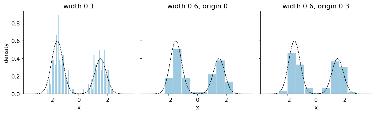
Divide the axis into bins of width and set for in bin with count . Histograms are simple and fast, but have three weaknesses visible in Figure 2. The estimate is discontinuous at bin edges. It depends on the origin of the grid as well as the width: shifting all bins by changes the picture. And in dimensions the number of bins grows like , so most bins are empty long before reaches ten. Scott’s analysis [8] shows that the bin width minimizing the mean integrated squared error shrinks only like , so more data buy finer bins slowly.
Parzen windows and kernel density estimation
The Parzen window or kernel density estimate (KDE), introduced by Rosenblatt [5] and analysed by Parzen [6], centers a window on every sample instead of fixing a grid:
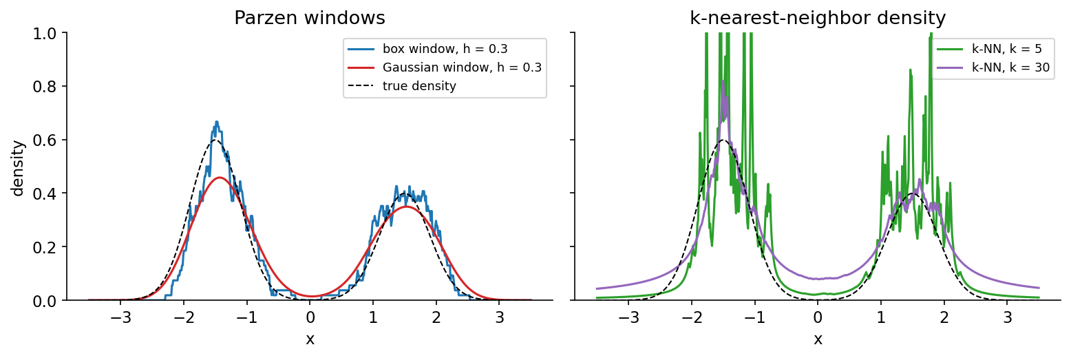
Here is the kernel, a function with and (so is a valid density), and is the bandwidth, which plays the role of the bin width. With a box kernel ( inside the unit cube) the formula is literally “count the samples within a cube of side around ”, the fixed- estimator above. A Gaussian kernel replaces the hard count with a smooth weight, giving a smooth estimate (Figure 3, left). In practice the shape of the kernel matters much less than the bandwidth.
Bias and variance. For a smooth density in one dimension, the bias of a KDE grows like (times the curvature ) and the variance like . Minimizing their sum gives an optimal bandwidth proportional to and a mean integrated squared error that falls like , slower than the of a correctly specified parametric model [7, 8]. In dimensions the optimal bandwidth scales like and the error like . The slowdown with is one face of the curse of dimensionality.
Choosing the bandwidth. This is the important practical decision. Common options:
- Rules of thumb. Silverman’s rule [7], where is the sample standard deviation and IQR the interquartile range, is optimal if the data are Gaussian. For multimodal data it oversmooths.
- Cross-validation. Choose to maximize the log-likelihood of held-out samples (likelihood cross-validation), or to minimize an unbiased estimate of the integrated squared error (least-squares cross-validation, analysed by Scott and Terrell [9]).
- Plug-in methods. Sheather and Jones [10] estimate the unknown curvature term in the optimal-bandwidth formula from the data and plug it in; their selector is a widely used reliable default in one dimension.
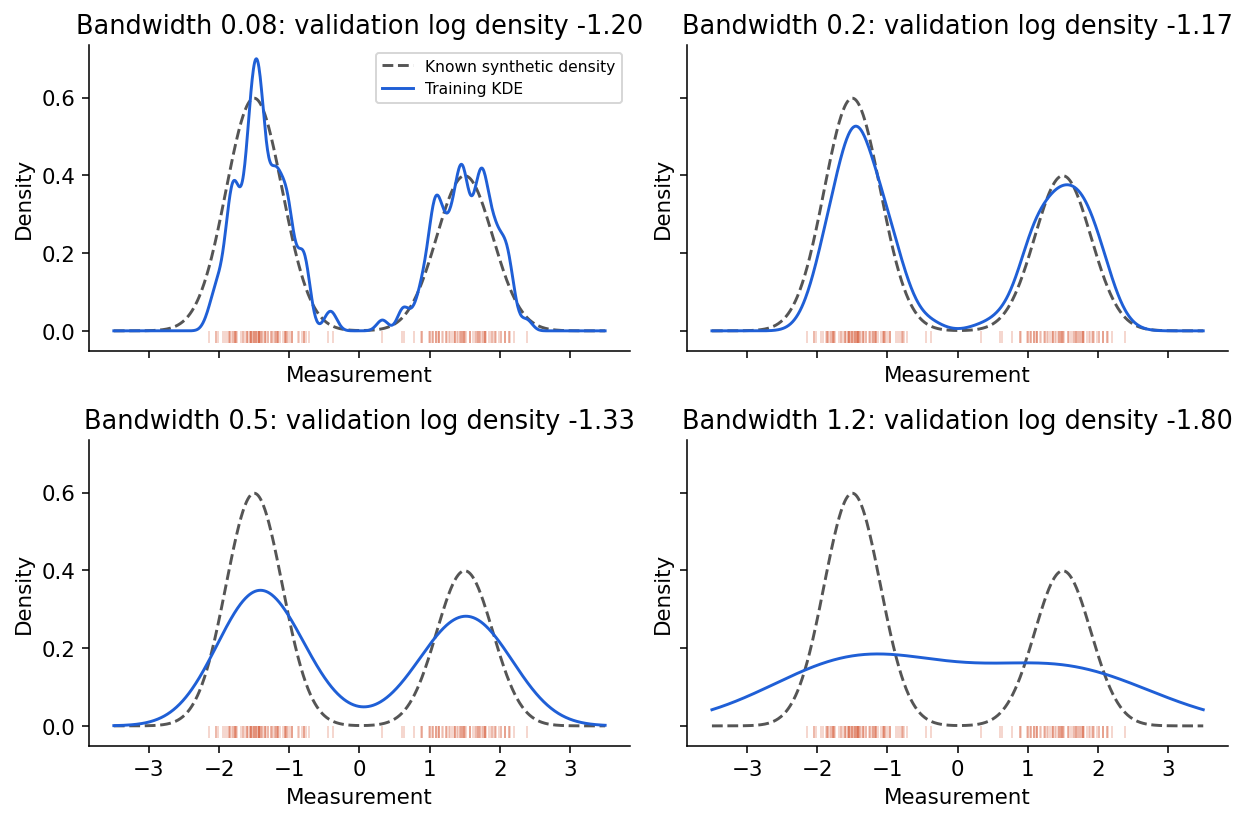
Whatever rule you use, choose without looking at the final test data. Figure 4 shows why the choice matters: on a bimodal sample, produces spurious bumps, merges the two modes into one, and the validation log-likelihood correctly prefers .
Code: bandwidth selection and a Beta posterior
This example uses scikit-learn’s KernelDensity [26] on a synthetic bimodal distribution, separate validation samples, Silverman’s rule for comparison, and the closed-form Beta posterior from the previous section.
Code · Python · 28 lines
import numpy as np
from scipy.stats import beta
from sklearn.neighbors import KernelDensity

rng = np.random.default_rng(4)
def sample(n):
    means = np.where(rng.random(n) < 0.6, -1.5, 1.5)
    return (means + rng.normal(0, 0.4, n)).reshape(-1, 1)
train, validation = sample(180), sample(100)
bandwidths = [0.08, 0.2, 0.5, 1.2]
scores = []
for h in bandwidths:
    model = KernelDensity(bandwidth=h).fit(train)
    scores.append(model.score(validation) / len(validation))
best = bandwidths[int(np.argmax(scores))]

# Silverman's rule of thumb for comparison
x = train.ravel()
iqr = np.subtract(*np.percentile(x, [75, 25]))
h_silverman = 0.9 * min(x.std(ddof=1), iqr / 1.34) * len(x) ** (-1 / 5)

posterior = beta(2, 1)  # uniform prior + one success
print("validation mean log densities:",
      {h: round(float(s), 3) for h, s in zip(bandwidths, scores)})
print("selected bandwidth:", best, "| Silverman's rule:", round(h_silverman, 3))
print("posterior mean:", posterior.mean())
print("95% credible interval:", posterior.ppf([0.025, 0.975]))
assert np.isclose(posterior.mean(), 2 / 3)
Validation selects , while Silverman’s rule gives . The rule assumes a single Gaussian; the spread of this sample comes mostly from the gap between the two modes, so the rule oversmooths. The Beta posterior after one success under a uniform prior has mean and a credible interval of roughly : one observation tells us very little.
A credible interval describes uncertainty under the assumed prior and likelihood; it is not automatically a calibrated frequentist coverage guarantee. Likewise, a good density score does not by itself guarantee a good classification boundary: some of the modelled variation may be irrelevant to the labels.
-nearest-neighbor density estimation
Fix instead of : around , grow a ball until it contains exactly samples, and let be its volume. Then [11]
Loftsgaarden and Quesenberry [11] showed that this estimate is consistent when and . Its bandwidth adapts automatically: narrow where data are dense, wide where they are sparse. But Figure 3 (right) shows its flaws. For small it is very spiky, because is tiny near clusters of samples. In the tails, grows only linearly with the distance in 1-D, so decays like , and the estimate does not integrate to one (its integral diverges). It is therefore a poor density estimate, yet, as the next section shows, an excellent basis for classification.
The -nearest-neighbor classifier
Plain version. To classify a new point, find the training points closest to it and take a majority vote. No model is trained; the training set is the model.
Precise version. Draw a ball around that contains samples in total, of which belong to class . Applying the estimate separately to each class, with samples in class , gives
The volume cancels, and the posterior estimate is simply the fraction of neighbors from each class. The Bayes rule then becomes the majority vote. With it is the nearest-neighbor rule.
How good is it? Cover and Hart [12] proved that, as , the error of the 1-NN rule satisfies
where is the Bayes error and the number of classes. This is an error-rate bound under the theorem’s sampling assumptions, not a statement that a neighbor contains half the information in the information-theoretic sense. As grows (with ), the -NN error approaches itself. This is an asymptotic statement; with finite data and many dimensions, things are much less rosy.
Choosing . Small gives low bias but high variance: the 1-NN boundary in Figure 5 wraps around individual noisy points. Large smooths the boundary but eventually ignores real structure. Choose by cross-validation. Two practical details: use an odd for two classes to avoid ties, and standardize the features first, because the Euclidean distance is dominated by whichever feature has the largest numeric range. In PR 04, kernels and nearest neighbors are compared with other nonlinear classifiers, and learned distance metrics are discussed there and in later chapters.
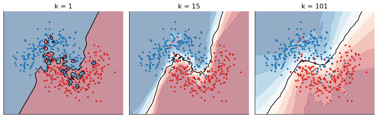
Code: k-NN versus Gaussian classifiers
Code · Python · 21 lines
import numpy as np
from sklearn.datasets import make_moons
from sklearn.model_selection import GridSearchCV, train_test_split
from sklearn.naive_bayes import GaussianNB
from sklearn.neighbors import KNeighborsClassifier
from sklearn.discriminant_analysis import QuadraticDiscriminantAnalysis

X, y = make_moons(1000, noise=0.3, random_state=0)
Xtr, Xte, ytr, yte = train_test_split(X, y, test_size=0.5, random_state=0)

search = GridSearchCV(KNeighborsClassifier(),
                      {"n_neighbors": [1, 3, 5, 9, 15, 31, 61, 101]}, cv=5)
search.fit(Xtr, ytr)                     # k chosen on training folds only
print("cross-validated k:", search.best_params_["n_neighbors"])
models = {"1-NN": KNeighborsClassifier(1),
          f"{search.best_params_['n_neighbors']}-NN": search.best_estimator_,
          "Gaussian naive Bayes": GaussianNB(),
          "QDA": QuadraticDiscriminantAnalysis()}
for name, m in models.items():
    m.fit(Xtr, ytr)
    print(f"{name:22s} test error {1 - m.score(Xte, yte):.3f}")
Cross-validation picks , with a test error of , against for 1-NN. The Gaussian models, whose single-ellipse class shapes cannot follow the moons, are worse ( for naive Bayes, for QDA). On this 2-D problem, the non-parametric method wins because the parametric form is wrong. The next section shows why the advantage shrinks as dimension grows.
The curse of dimensionality
Plain version. Local methods need neighbors that are close. When many coordinates contain diffuse or irrelevant variation, distance can become a poor guide: to collect even a small fraction of the data you must reach across most of the space, and the nearest and farthest points end up at almost the same distance.
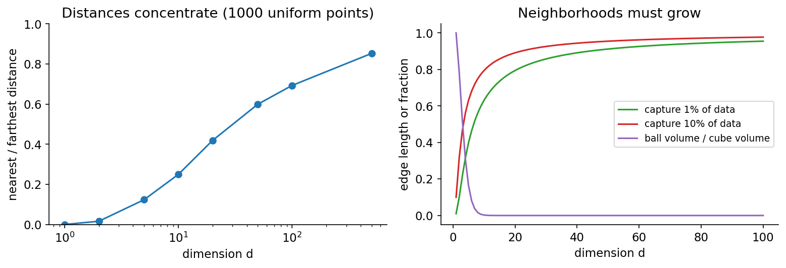
Precise version. The phrase “curse of dimensionality” covers several related effects; Bishop [2, Section 1.4] gives geometric illustrations. Three are easy to check (Figure 6):
- Neighborhoods must be huge. For data uniform in the unit cube , a sub-cube that contains a fraction of the data has edge length . To capture of the data, the edge is in 2-D, in 10-D and in 100-D. A “local” neighborhood spans almost the full range of every feature, so the estimate is no longer local.
- Volume is in the corners and the shell. The volume of the unit ball divided by the volume of its enclosing cube tends to zero rapidly, and for a ball almost all volume lies in a thin shell near its surface. Samples from high-dimensional Gaussians sit at nearly the same distance from the mean, not near it.
- Distances concentrate. Beyer et al. [13] proved that, under broad conditions on the data distribution, the ratio of the farthest to the nearest neighbor distance tends to one as grows, so “nearest neighbor” stops being meaningful. In the simulation below, the ratio of nearest to farthest distance rises from in 2-D to about in 100-D.
Code: distance concentration
Code · Python · 11 lines
import numpy as np

rng = np.random.default_rng(0)
for d in [1, 2, 10, 100, 1000]:
    pts = rng.random((1000, d))          # 1000 uniform points in [0, 1]^d
    q = rng.random((50, d))              # 50 query points
    dist = np.sqrt(((q[:, None, :] - pts[None]) ** 2).sum(-1))
    ratio = (dist.min(1) / dist.max(1)).mean()
    edge = 0.1 ** (1 / d)                # sub-cube edge holding 10% of the volume
    print(f"d={d:5d}: nearest/farthest = {ratio:.3f}, "
          f"edge for 10% of data = {edge:.3f}")
The nearest/farthest ratio is in 2-D, in 10-D, in 100-D and in 1000-D.
Why does anything work in high dimensions, then? Real data are not uniform. Images, sounds and text lie close to low-dimensional structures (manifolds, clusters) inside their huge ambient spaces, and their informative directions are far fewer than their raw coordinates. Practical defences are therefore: reduce or learn the representation first (PR 05: features and dimensionality), constrain the model (shared or diagonal covariances, naive Bayes), and regularize. Nearest-neighbor methods work very well today precisely because they are applied to learned embeddings rather than raw pixels, as the Modern view explains.
Modern view
Density estimation has split into two streams since the textbooks were written: classical statistics refined KDE and covariance estimation, while deep learning built density models that scale to images, and nearest-neighbor search became infrastructure.
Kernel density estimation, revisited. Chen’s tutorial [16] is a gentle modern introduction: convergence rates, bandwidth selection, confidence bands and how to handle their bias, and recent work on estimating geometric and topological features of a density (modes, level sets, ridges) with KDE. Wang and Scott [17] review non-parametric density estimators designed for high-dimensional data, including applications such as modal clustering, and list open research directions. Scott’s monograph [8] and Silverman’s classic [7] remain the references for the theory.
High-dimensional covariance. The singular-covariance problem of this chapter is a whole research area. Fan, Liao and Liu [18] review estimators of large covariance and precision (inverse covariance) matrices, focusing on rank-based methods and factor-model-based methods; Ledoit–Wolf shrinkage [14] is still the default regularizer in libraries.
Deep density models. Normalizing flows build a flexible density by passing a simple base distribution through a chain of invertible, differentiable maps; the change-of-variables formula then gives an exact log-likelihood. Papamakarios et al. [19] and Kobyzev, Prince and Brubaker [20] are the two standard reviews: the first emphasizes design principles, expressive power and computational trade-offs, the second the construction of flows and open questions. Autoregressive models, VAEs and diffusion models are other ways to learn high-dimensional densities; see ML 07: generative models and ML 08: diffusion and flow matching. Murphy’s two-volume text [4] covers both the classical estimators of this chapter and these modern models in one notation.
Nearest neighbors at scale. -NN is now everywhere, but on learned embeddings instead of raw features. Johnson, Douze and Jégou [21] showed how to run billion-scale similarity search on GPUs, and the Faiss library paper [22] describes the trade-off space of vector search (accuracy, speed, memory) and the indexing methods behind modern vector databases. Papernot and McDaniel’s deep -NN [23] compares a test input with its training neighbors in every layer’s representation, using label disagreement among neighbors as a confidence and robustness signal. For out-of-distribution detection, Sun et al. [24] use the plain -th nearest-neighbor distance in feature space, without any distributional assumption, and report large improvements over a parametric Mahalanobis-distance baseline. That parametric baseline, from Lee et al. [25], fits class-conditional Gaussians with shared covariance to network features, which is LDA from PR 01. The parametric versus non-parametric choice of this chapter is being replayed on top of deep features.
Open problems. Reliable density estimation in high dimension remains hard. Nalisnick et al. [27] showed that flow-based models, VAEs and PixelCNNs trained on one image dataset can assign higher likelihood to a different dataset (for example, a model trained on a dataset of everyday objects scores a dataset of house-number photos higher), so likelihood alone is not a safe novelty score. Bandwidth or selection for embeddings, and calibrated uncertainty for non-parametric estimates, are active questions.
Key takeaways
- Generative classifiers need and ; the estimator’s assumptions decide the boundary’s shape.
- ML estimates for a Gaussian are the sample mean and the divisor- covariance; with samples the covariance is singular, and shrinkage (e.g. Ledoit–Wolf) or shared/diagonal structure is needed.
- MAP keeps the posterior mode; full Bayesian prediction integrates over parameters and is wider than plug-in prediction when data are scarce. Conjugate priors give closed forms: precisions add for a Gaussian mean, counts add for a Beta–Bernoulli rate.
- Non-parametric estimates all follow from : histograms and Parzen/KDE fix , -NN fixes . The bandwidth or matters more than the kernel; choose it by cross-validation or a justified rule, never on test data.
- The -NN classifier estimates ; asymptotically 1-NN is within a factor two of the Bayes error.
- In high dimensions neighborhoods stop being local and distances concentrate; whether local methods work depends on intrinsic structure, feature scaling and sample size, not ambient dimension alone.
Exercises
- Counting parameters. Count the mean and covariance parameters of one 64-dimensional Gaussian. Explain why fitting it to 30 samples fails, and give two ways to fix it.
Hint
means plus covariance entries. With 30 samples, has rank at most 29, so it is singular. Fixes: shrinkage towards (Ledoit–Wolf), a diagonal covariance (naive Bayes), a covariance shared across classes, or dimensionality reduction first.
- Beta–Bernoulli update. Start with , observe three successes and two failures, and compute the posterior, the MAP estimate and the posterior predictive probability of success.
Hint
Posterior . MAP (mode) . Predictive . Compare with ML, .
- Precision-weighted means. For the Gaussian mean with prior and noise variance , after how many samples does the data weight equal the prior weight? What is the posterior standard deviation then?
Hint
Prior precision ; each sample adds . Equal weight at . Posterior precision , so .
- Duplicated features. Duplicate one feature in Gaussian naive Bayes. Predict what happens to accuracy and to the confidence of the posteriors, then check with scikit-learn on
load_breast_cancer.
Hint
The extra coordinate adds no new information, but the factorized likelihood counts it twice, squaring its likelihood ratio. Decisions may change a little; posteriors move closer to 0 or 1 (more overconfident). Compare predict_proba histograms and the log-loss before and after.
- k-NN density is not a density. Show that in 1-D the -NN estimate decays like far from the data, and conclude that diverges. Why does this not hurt the -NN classifier?
Hint
Far from all samples, the distance to the -th neighbor is about , so and , whose integral is logarithmically divergent. The classifier only uses ratios at the same point, where the common volume cancels.
- Bandwidth rules. Generate 500 samples from a mixture of and . Compare Silverman’s rule, likelihood cross-validation (
GridSearchCVoverKernelDensity) and, if you havestatsmodels, a plug-in selector. Which oversmooths, and why?
Hint
Silverman’s rule uses the overall spread (about here), which is dominated by the gap between the modes, so it gives a bandwidth several times too large for each mode. Cross-validated likelihood picks something close to the within-mode optimum.
References
- R. O. Duda, P. E. Hart and D. G. Stork, Pattern Classification, 2nd ed., Wiley, 2001 (Ch. 3, maximum-likelihood and Bayesian estimation; Ch. 4, non-parametric techniques). publisher page
- C. M. Bishop, Pattern Recognition and Machine Learning, Springer, 2006 (Sections 1.4, 2.1–2.3, 2.5 and 4.2). official page and free PDF
- S. Theodoridis and K. Koutroumbas, Pattern Recognition, 4th ed., Academic Press, 2008 (Ch. 2, density estimation and Bayesian classification). publisher page
- K. P. Murphy, Probabilistic Machine Learning: An Introduction, MIT Press, 2022. official page
- M. Rosenblatt, “Remarks on some nonparametric estimates of a density function,” The Annals of Mathematical Statistics, vol. 27, no. 3, pp. 832–837, 1956. doi
- E. Parzen, “On estimation of a probability density function and mode,” The Annals of Mathematical Statistics, vol. 33, no. 3, pp. 1065–1076, 1962. doi
- B. W. Silverman, Density Estimation for Statistics and Data Analysis, Chapman and Hall, 1986 (reissued by Routledge, 2018). doi
- D. W. Scott, Multivariate Density Estimation: Theory, Practice, and Visualization, 2nd ed., Wiley, 2015. doi
- D. W. Scott and G. R. Terrell, “Biased and unbiased cross-validation in density estimation,” Journal of the American Statistical Association, vol. 82, no. 400, pp. 1131–1146, 1987. doi
- S. J. Sheather and M. C. Jones, “A reliable data-based bandwidth selection method for kernel density estimation,” Journal of the Royal Statistical Society, Series B, vol. 53, no. 3, pp. 683–690, 1991. doi
- D. O. Loftsgaarden and C. P. Quesenberry, “A nonparametric estimate of a multivariate density function,” The Annals of Mathematical Statistics, vol. 36, no. 3, pp. 1049–1051, 1965. doi
- T. M. Cover and P. E. Hart, “Nearest neighbor pattern classification,” IEEE Transactions on Information Theory, vol. 13, no. 1, pp. 21–27, 1967. doi
- K. Beyer, J. Goldstein, R. Ramakrishnan and U. Shaft, “When is ‘nearest neighbor’ meaningful?,” in Database Theory — ICDT’99, Lecture Notes in Computer Science, Springer, 1999. doi
- O. Ledoit and M. Wolf, “A well-conditioned estimator for large-dimensional covariance matrices,” Journal of Multivariate Analysis, vol. 88, no. 2, pp. 365–411, 2004. doi
- A. Y. Ng and M. I. Jordan, “On discriminative vs. generative classifiers: a comparison of logistic regression and naive Bayes,” in Advances in Neural Information Processing Systems (NIPS), 2001. paper
- Y.-C. Chen, “A tutorial on kernel density estimation and recent advances,” Biostatistics & Epidemiology, vol. 1, no. 1, pp. 161–187, 2017. doi
- Z. Wang and D. W. Scott, “Nonparametric density estimation for high-dimensional data — algorithms and applications,” WIREs Computational Statistics, vol. 11, no. 4, 2019. doi
- J. Fan, Y. Liao and H. Liu, “An overview of the estimation of large covariance and precision matrices,” The Econometrics Journal, vol. 19, no. 1, pp. C1–C32, 2016. doi
- G. Papamakarios, E. Nalisnick, D. J. Rezende, S. Mohamed and B. Lakshminarayanan, “Normalizing flows for probabilistic modeling and inference,” Journal of Machine Learning Research, vol. 22, no. 57, pp. 1–64, 2021. arXiv
- I. Kobyzev, S. J. D. Prince and M. A. Brubaker, “Normalizing flows: an introduction and review of current methods,” IEEE Transactions on Pattern Analysis and Machine Intelligence, vol. 43, no. 11, pp. 3964–3979, 2021. doi
- J. Johnson, M. Douze and H. Jégou, “Billion-scale similarity search with GPUs,” IEEE Transactions on Big Data, vol. 7, no. 3, pp. 535–547, 2021. doi
- M. Douze, A. Guzhva, C. Deng, J. Johnson, G. Szilvasy, P.-E. Mazaré, M. Lomeli, L. Hosseini and H. Jégou, “The Faiss library,” arXiv:2401.08281, 2024. arXiv
- N. Papernot and P. McDaniel, “Deep k-nearest neighbors: towards confident, interpretable and robust deep learning,” arXiv:1803.04765, 2018. arXiv
- Y. Sun, Y. Ming, X. Zhu and Y. Li, “Out-of-distribution detection with deep nearest neighbors,” in Proc. International Conference on Machine Learning (ICML), PMLR 162, 2022. paper
- K. Lee, K. Lee, H. Lee and J. Shin, “A simple unified framework for detecting out-of-distribution samples and adversarial attacks,” in Advances in Neural Information Processing Systems (NeurIPS), 2018. paper
- scikit-learn developers, “Density estimation,” scikit-learn user guide. documentation
- E. Nalisnick, A. Matsukawa, Y. W. Teh, D. Gorur and B. Lakshminarayanan, “Do deep generative models know what they don’t know?,” in Proc. International Conference on Learning Representations (ICLR), 2019. arXiv
Check your understanding
This tutorial has 6 exercises. Can you solve them without opening the hints?
Go to the exercises ↑Next PR 03 · Linear Models for Regression and Classification · 23 min