PR 06 · Template Matching and Structured Recognition
Needs: PR 05 · Feature Selection, Transforms and Dimensionality
Navigate: this page and this track: Navigate: this page and this track
On this page
- What you’ll learn1 min
- The big picture1 min
- Template matching3 min
- Dynamic time warping3 min
- Syntactic and structural pattern recognition3 min
- Graphical models describe dependence1 min
- Hidden Markov models5 min
- Conditional random fields2 min
- Modern view3 min
- Key takeaways1 min
- Exercises2 min
- Supplementary notes
- References
Pattern Recognition
Explore this chapter 1 interactive experiment
Warp a signal in time and inspect a dynamic time warping cost matrix and its optimal alignment path.
What you’ll learn
- How template matching works with sum of squared differences, cross-correlation and normalized cross-correlation (NCC), and which nuisance changes each one tolerates.
- How dynamic time warping (DTW) aligns sequences that unfold at different speeds, and how to constrain it.
- Syntactic and structural pattern recognition: describing patterns as strings, grammars and graphs, and comparing them with edit distance and graph matching.
- How directed and undirected graphical models factorize a joint distribution, and why that makes inference efficient.
- Hidden Markov models: the forward algorithm, forward–backward smoothing, Viterbi decoding and Baum–Welch learning, with tested code.
- Conditional random fields as the discriminative counterpart of HMMs, and where all of these ideas live on in 2026.
The big picture
The classifiers of PR 03 and PR 04 look at one fixed-length feature vector at a time and decide its class alone. Many recognition problems are not like that:
- To find a part in an image, you slide a reference picture over the image and look for the best match (templates).
- A spoken word or a signature unfolds in time, and two people produce it at different speeds (alignment).
- A character, a molecule or a road network is best described by its parts and how they connect (structure).
- An isolated image patch might be road or roof; a blurry handwritten letter might be “c” or “e”. Neighboring regions or letters resolve the ambiguity (context).
A common thread runs through the whole chapter: dynamic programming. DTW, edit distance, the HMM forward algorithm, Viterbi decoding and CRF inference are all the same trick. Break a huge search over all alignments or label sequences into small, reusable subproblems, and the cost drops from exponential to polynomial.
One caution belongs at the start. Context helps only when its assumptions match reality. A strong “neighbors agree” rule can erase small objects or brief events, so more context is not automatically better. The textbook background is Theodoridis and Koutroumbas, Chapters 8 and 9 [1], and Bishop, Sections 8.1–8.4 and 13.1–13.3 [2].
Template matching
In plain words. Keep a small reference image, the template. Slide it over the scene, and at every position measure how similar the patch underneath is. The best-scoring position is the match. The interesting question is how to measure similarity so that irrelevant changes, such as a brighter or dimmer exposure, do not fool you.
Three similarity measures
Write the template as a vector of its pixel values and the image patch under it as , also of length .
Sum of squared differences (SSD). . Small is good. It is the natural distance, but any brightness offset or contrast change in the scene increases it.
Cross-correlation. Expanding the square, . The template energy is constant, so if the patch energy were roughly constant too, minimizing SSD would be the same as maximizing the correlation . In practice varies a lot, and plain correlation is drawn to bright regions.
Normalized cross-correlation (NCC). Subtract the means and divide by the norms:
where and are the mean pixel values of the patch and the template and is the all-ones vector. NCC is the cosine of the angle between the mean-subtracted vectors, so it lies in , and it equals 1 exactly when for some and any . It is therefore invariant to positive changes of contrast () and to brightness offsets (). It is undefined for a constant template or patch (zero denominator); implementations return a convention such as 0 or NaN. NCC is the “matching by correlation” of IP 13.
Computing it efficiently
Evaluating NCC at every position of an image with an template costs on the order of operations. The numerator is a correlation, which can be computed for all positions at once with the FFT (the correlation theorem, IP 04). The local means and energies in the denominator vary from position to position; Lewis showed how to get them cheaply from running-sum tables (integral images) of the image and of its square, which makes NCC nearly as fast as plain correlation [3].
Code · Python · 22 lines
import cv2
import numpy as np
from skimage import data

img = data.camera().astype(np.float32)          # 512 x 512 grayscale
r0, c0, h, w = 300, 200, 40, 40
template = img[r0:r0 + h, c0:c0 + w].copy()

def ncc_at(window, t):
    a, b = window - window.mean(), t - t.mean()
    return float((a * b).sum() / (np.linalg.norm(a) * np.linalg.norm(b)))

# The scene is captured again under different exposure: darker and lower contrast.
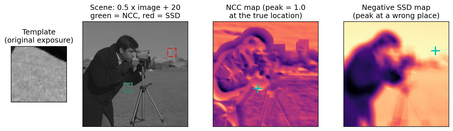
scene = 0.5 * img + 20.0
ncc = cv2.matchTemplate(scene, template, cv2.TM_CCOEFF_NORMED)
ssd = cv2.matchTemplate(scene, template, cv2.TM_SQDIFF)
r, c = np.unravel_index(ncc.argmax(), ncc.shape)
print("NCC best (row, col):", (int(r), int(c)), "score", round(float(ncc.max()), 4))
r, c = np.unravel_index(ssd.argmin(), ssd.shape)
print("SSD best (row, col):", (int(r), int(c)))
print("hand-computed NCC at true location:",
      round(ncc_at(scene[r0:r0 + h, c0:c0 + w], template), 4))
NCC finds the template at its true position (300, 200) with a score of 1.0, and the hand-computed value agrees with OpenCV’s TM_CCOEFF_NORMED. SSD, fooled by the exposure change, picks (130, 413), a patch of sky whose darkened intensities (mean about 129) are closer to the template’s original values (mean about 143) than the darkened true patch is (mean about 92).
What templates cannot handle
NCC removes brightness and contrast, nothing else. Rotation, scale change, perspective, occlusion and non-rigid deformation all lower the score. The classical remedies are to store a family of templates (rotated and scaled copies), to search over an image pyramid, or to match small parts and then check their geometric arrangement, which leads to the structural methods below. Template matching remains the right tool when appearance is tightly controlled, as in industrial inspection, and it is still a core step in tracking and image registration [4].
Dynamic time warping
In plain words. Two people say the same word, one slowly, one quickly. Comparing the recordings sample by sample fails because the sounds do not line up in time. DTW stretches and compresses the time axis of one sequence to line it up with the other as well as possible, then measures the remaining difference.
The recursion
Let and be two sequences, and a local cost such as or for vector-valued samples. A warping path is a sequence of index pairs that starts at , ends at , and moves by one of the steps , or at a time, so that it never goes backward in either sequence. DTW is the smallest total cost over all warping paths. It is computed by filling a table:
with and for . Then . Each cell needs only its three neighbors, so the cost is time. Tracing back which neighbor gave the minimum recovers the optimal alignment. This is the algorithm Sakoe and Chiba optimized for spoken-word recognition [5].
Constraints and caveats
An unconstrained path can match a single sample of one sequence to a long stretch of the other (“pathological warping”), which lets unrelated sequences look similar. Two standard fixes are:
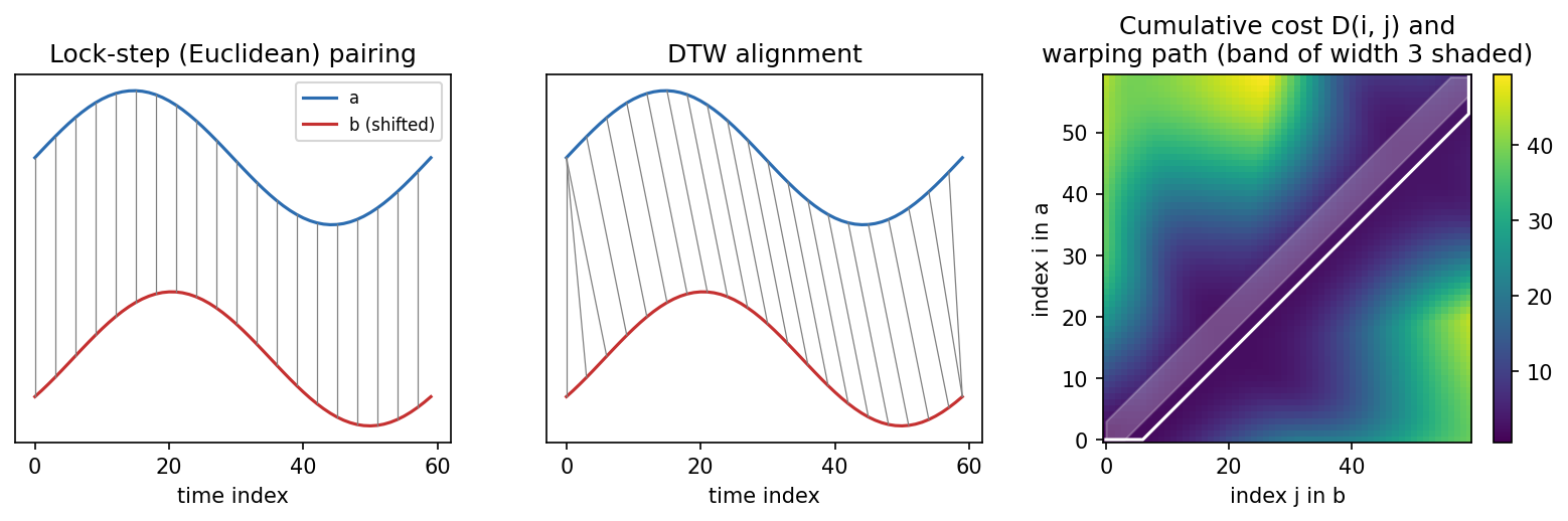
- a global constraint, such as the Sakoe–Chiba band , which forbids cells far from the diagonal and also reduces the cost to [5];
- slope constraints or step weights that penalize long horizontal or vertical runs [5].
The band width must allow the real timing differences. In the code and in Figure 2, a band of 3 samples is narrower than the true shift of about 6 samples, so the banded DTW cannot fully align the two sine waves.
Two further facts matter in practice. DTW is not a metric: it can violate the triangle inequality, so data structures that assume a metric need care. And sequences are usually z-normalized (zero mean, unit variance) before comparison, so that DTW compares shapes rather than offsets and scales.
Code · Python · 25 lines
import numpy as np

def dtw(x, t, band=None):
    """DTW distance between 1-D sequences x (length n) and t (length m)."""
    n, m = len(x), len(t)
    D = np.full((n + 1, m + 1), np.inf)
    D[0, 0] = 0.0
    for i in range(1, n + 1):
        lo, hi = 1, m
        if band is not None:                    # Sakoe-Chiba band
            lo, hi = max(1, i - band), min(m, i + band)
        for j in range(lo, hi + 1):
            cost = abs(x[i - 1] - t[j - 1])
            D[i, j] = cost + min(D[i - 1, j], D[i, j - 1], D[i - 1, j - 1])
    return D[n, m]

s = np.linspace(0, 2 * np.pi, 60)
a = np.sin(s)
b = np.sin(s - 0.6)                              # same shape, shifted in time
c = 0.25 * np.sign(np.sin(3 * s))                # a different shape
print("lock-step a-b:", round(np.abs(a - b).sum(), 2),
      " a-c:", round(np.abs(a - c).sum(), 2))
print("DTW       a-b:", round(dtw(a, b), 2),
      " a-c:", round(dtw(a, c), 2))
print("DTW a-b with band 3:", round(dtw(a, b, band=3), 2))
Both comparisons use the same local cost . Sample by sample (“lock-step”), the shifted copy costs 22.76 and the different shape costs 35.18. DTW reduces the shifted copy to 5.05 while the different shape stays at 34.57: warping absorbs timing differences, not shape differences. With a band of 3 samples, the cost of the shifted copy rises to 12.76 because the band is too narrow for a shift of about 6 samples.
A 1-nearest-neighbor classifier with DTW distance was for many years a strong, hard-to-beat baseline for time-series classification [16]. Searching for the nearest neighbor under DTW in very long series became practical once cheap lower bounds and early abandoning of hopeless candidates were combined [6].
Syntactic and structural pattern recognition
In plain words. Some patterns are best described not by a list of numbers but by their parts and how the parts fit together, the way a sentence is words arranged by grammar. Structural pattern recognition describes a pattern as a string, tree or graph of primitive parts, and compares or parses those structures.
Strings and grammars
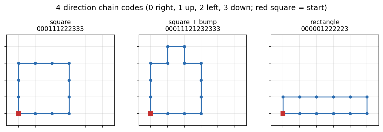
Choose a small alphabet of primitives, for example the four directions of a step along an object’s boundary. Then a shape becomes a string. A 4-direction chain code writes 0 for a step right, 1 up, 2 left and 3 down while tracing the boundary (see IP 12). Figure 3 shows three outlines and their codes.
In syntactic pattern recognition each class is described by a formal grammar: a set of rewrite rules that generates exactly the valid strings of that class. Recognition is parsing: a string belongs to a class if that class’s grammar can generate it. For example, the rule set generates strings , a “class” in which every rightward run is matched by an equally long leftward run. Grammars can express recursive structure (nested parts, repeated sub-shapes) that fixed-length feature vectors cannot. Their weaknesses are that real data are noisy, so a single wrong primitive makes a string ungrammatical, and that grammars are hard to learn from examples. Stochastic grammars, which attach probabilities to rules, address the first problem; a hidden Markov model, below, is the simplest stochastic grammar of all [1].
Edit distance
A more forgiving approach compares strings by the cheapest way to turn one into the other. The edit distance (Levenshtein distance) counts the minimum number of insertions, deletions and substitutions. Wagner and Fischer gave the dynamic program [7]:
with and , for strings (length ) and (length ); the answer is . The structure is exactly that of DTW, with the operations “insert”, “delete” and “substitute” instead of “stretch”. Costs can be weighted, for example to make substituting neighboring directions cheaper than opposite ones.
Code · Python · 22 lines
import numpy as np

def edit_distance(s, t):
    """Levenshtein distance: unit-cost insertions, deletions, substitutions."""
    n, m = len(s), len(t)
    D = np.zeros((n + 1, m + 1), dtype=int)
    D[:, 0] = np.arange(n + 1)
    D[0, :] = np.arange(m + 1)
    for i in range(1, n + 1):
        for j in range(1, m + 1):
            sub = 0 if s[i - 1] == t[j - 1] else 1
            D[i, j] = min(D[i - 1, j] + 1,          # delete s[i-1]
                          D[i, j - 1] + 1,          # insert t[j-1]
                          D[i - 1, j - 1] + sub)    # match or substitute
    return D[n, m]

# 4-direction chain codes (0=right, 1=up, 2=left, 3=down) of three outlines
square = "000111222333"           # 3 x 3 square, traced counter-clockwise
square_bump = "00011121232333"   # the same square with a one-pixel bump on top
rectangle = "000001222223"       # a flat 5 x 1 rectangle
for name, code in [("square + bump", square_bump), ("rectangle", rectangle)]:
    print(f"edit distance(square, {name}) = {edit_distance(square, code)}")
The bumped square is 2 edits from the square (insert one “up” and one “down”); the flat rectangle is 4 edits away. A nearest-neighbor classifier over strings with this distance is the structural analogue of -NN. Chain codes depend on the starting point and on rotation; normalizing them (for example by choosing the starting point that gives the smallest string, and by using differences between successive directions) is part of the representation design.
Graphs and graph matching
When parts connect in more than a chain, a pattern becomes an attributed graph: nodes are parts (strokes, regions, atoms) with attributes such as size or color, and edges are relations (touching, above, bonded). Recognition then means graph matching: finding a correspondence between the nodes of two graphs. Exact matching (graph or subgraph isomorphism) tolerates no differences and is computationally hard in general; error-tolerant matching, such as graph edit distance, generalizes string edit distance with node and edge insertions, deletions and substitutions, at an even higher computational price. Conte, Foggia, Sansone and Vento surveyed three decades of graph matching in pattern recognition, from exact algorithms to inexact ones and their applications [8], and Foggia, Percannella and Vento updated the picture with a decade of graph matching and graph learning methods [9].
Graphical models describe dependence
In plain words. A graphical model is a drawing of which variables directly influence which. The drawing tells you how a huge joint probability breaks into small local pieces, and small pieces are what make computation possible.
A directed acyclic graph (a Bayesian network) factorizes the joint distribution of variables as
where are the parents of in the graph [2]. An undirected graph (a Markov random field) uses nonnegative potential functions on its cliques (fully connected subsets of nodes):
A potential is a compatibility score, not necessarily a probability. The partition function normalizes the product; it sums over all joint configurations and is often the hardest quantity to compute.
Conditional independence is read from the graph by its rules (d-separation for directed graphs, graph separation for undirected ones), not from the mere absence of an arrow. A classic surprise: two independent causes become dependent once you condition on their common effect (“explaining away”) [2]. Factor graphs draw variables and factors as two kinds of nodes and make local message passing explicit; on trees, message passing (the sum-product algorithm) computes all marginals exactly, and the HMM algorithms below are its special case on a chain [2].
For image labeling, a common undirected model is an energy with unary data terms and pairwise smoothness terms:
where is the label of pixel , is the cost of that label given the image (for example the negative log-probability from a pixel classifier), is the set of neighboring pixel pairs, and is the price of a label change between neighbors (a Potts model). The distribution is . It encourages neighboring labels to agree, which cleans up noise but can also erase thin structures if is too large. Exact minimization is hard on general grids, and PR 08 covers approximate inference.
Hidden Markov models
In plain words. A system moves between a few hidden states (silence, vowel, consonant; walking, running) and at each time step emits an observation that depends only on the current state. You see the observations, never the states. An HMM lets you compute how likely an observation sequence is, which hidden states probably produced it, and how to learn the model’s probabilities from data.
The model
An HMM with hidden states has initial probabilities , a transition matrix , and emission probabilities (or densities) . The joint probability of states and observations is
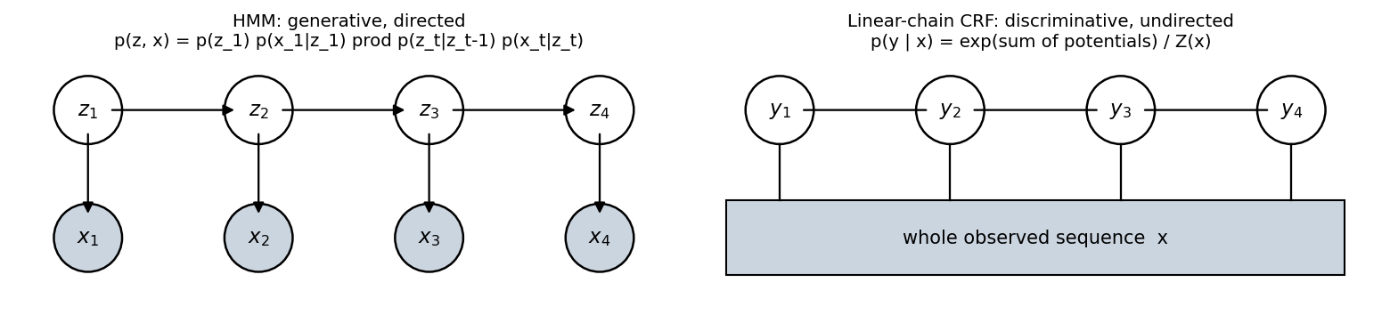
Two assumptions are built in: the hidden state is first-order Markov (the future depends on the past only through the present state), and each observation depends only on the current state. The observations themselves are not Markov: integrating out the hidden states creates long-range dependence among them. Rabiner’s tutorial, still the standard introduction, organizes HMM computation around three problems [10]: evaluation (compute ), decoding (find the hidden states) and learning (estimate ). Figure 4 contrasts the HMM’s directed graph with the CRF discussed later.
Evaluation: the forward algorithm
Summing the joint over all state sequences is hopeless for realistic . Define the forward variable . Because summarizes everything the past can tell about the future, it satisfies
and . The cost is instead of . Since is a product of many probabilities, it underflows for long sequences. The standard fix is to normalize at each step: store and , where is the unnormalized update. Then is exactly the filtered state probability, , and
Evaluation gives a classifier immediately: train one HMM per class (one per spoken word, say) and assign a new sequence to the class whose HMM gives it the highest likelihood, times the prior.
Smoothing: the forward–backward algorithm
Filtering computes from past and present only; it is what an online system can know at time . Smoothing computes , using later observations as well. A backward recursion ,
combines with the forward variable to give [2], [10]. With scaling, divide each backward step by , and then (elementwise product) exactly.
Decoding: the Viterbi algorithm
Often we want the single most probable sequence of states, . Viterbi’s algorithm [11] replaces the sum in the forward recursion by a maximum. In log space,
where is the log-probability of the best path that ends in state at time . Store the maximizing predecessor , pick the best final state, and trace the pointers backward. The cost is again .
The most probable path is not the same as choosing, at each time, the state with the highest smoothed probability . The per-step choice maximizes the expected number of correct states but can string together states that the model says cannot follow each other. The code shows this on a model whose states must cycle , so the transition has probability zero.
Code · Python · 57 lines
import itertools
import numpy as np

pi = np.array([1 / 3, 1 / 3, 1 / 3])            # initial state probabilities
A = np.array([[0.5, 0.5, 0.0],                  # cyclic model: 0 -> 1 -> 2 -> 0
              [0.0, 0.5, 0.5],
              [0.5, 0.0, 0.5]])
B = np.array([[0.7, 0.3],                       # P(symbol | state)
              [0.5, 0.5],
              [0.3, 0.7]])
obs = np.array([1, 0, 1, 0, 0])
T, K = len(obs), len(pi)

# Forward pass with scaling: alpha[t] = p(z_t | x_1..t), c[t] = p(x_t | x_1..t-1).
alpha, c = np.zeros((T, K)), np.zeros(T)
alpha[0] = pi * B[:, obs[0]]
c[0] = alpha[0].sum(); alpha[0] /= c[0]
for t in range(1, T):
    alpha[t] = B[:, obs[t]] * (alpha[t - 1] @ A)
    c[t] = alpha[t].sum(); alpha[t] /= c[t]
log_lik = np.log(c).sum()

# Backward pass (scaled) and smoothed marginals gamma[t] = p(z_t | x_1..T).
beta = np.ones((T, K))
for t in range(T - 2, -1, -1):
    beta[t] = A @ (B[:, obs[t + 1]] * beta[t + 1]) / c[t + 1]
gamma = alpha * beta

# Viterbi in log space (log 0 = -inf marks forbidden transitions).
with np.errstate(divide="ignore"):
    lA, lB, lpi = np.log(A), np.log(B), np.log(pi)
delta = lpi + lB[:, obs[0]]
back = []
for t in range(1, T):
    cand = delta[:, None] + lA
    back.append(cand.argmax(axis=0))
    delta = cand.max(axis=0) + lB[:, obs[t]]
path = [int(delta.argmax())]
for b in reversed(back):
    path.append(int(b[path[-1]]))
path = path[::-1]

# Brute force over all K**T paths as an independent check.
def joint(z):
    p = pi[z[0]] * B[z[0], obs[0]]
    for t in range(1, T):
        p *= A[z[t - 1], z[t]] * B[z[t], obs[t]]
    return p
paths = list(itertools.product(range(K), repeat=T))
assert np.isclose(log_lik, np.log(sum(joint(z) for z in paths)))
assert tuple(path) == max(paths, key=joint)

marginal = gamma.argmax(axis=1)
print("log p(x):", round(log_lik, 4))
print("Viterbi path:         ", path, " p =", round(joint(path), 5))
print("per-step argmax gamma:", marginal.tolist(),
      " p =", round(joint(marginal), 5))
The scaled forward pass gives , and both the likelihood and the Viterbi path agree with brute-force enumeration of all paths. Viterbi returns with joint probability 0.00179. Picking the most probable state at each step gives , which contains the forbidden jump and has probability exactly zero under the model. Which decoder is right depends on the loss: per-step accuracy favors the marginals; a valid, coherent sequence needs Viterbi.
Figure 5 shows the same computations on a longer simulated sequence: the filtered probabilities react only to the past, the smoothed ones use the whole sequence and are more confident, and the Viterbi path tracks the true states except where observations are ambiguous.
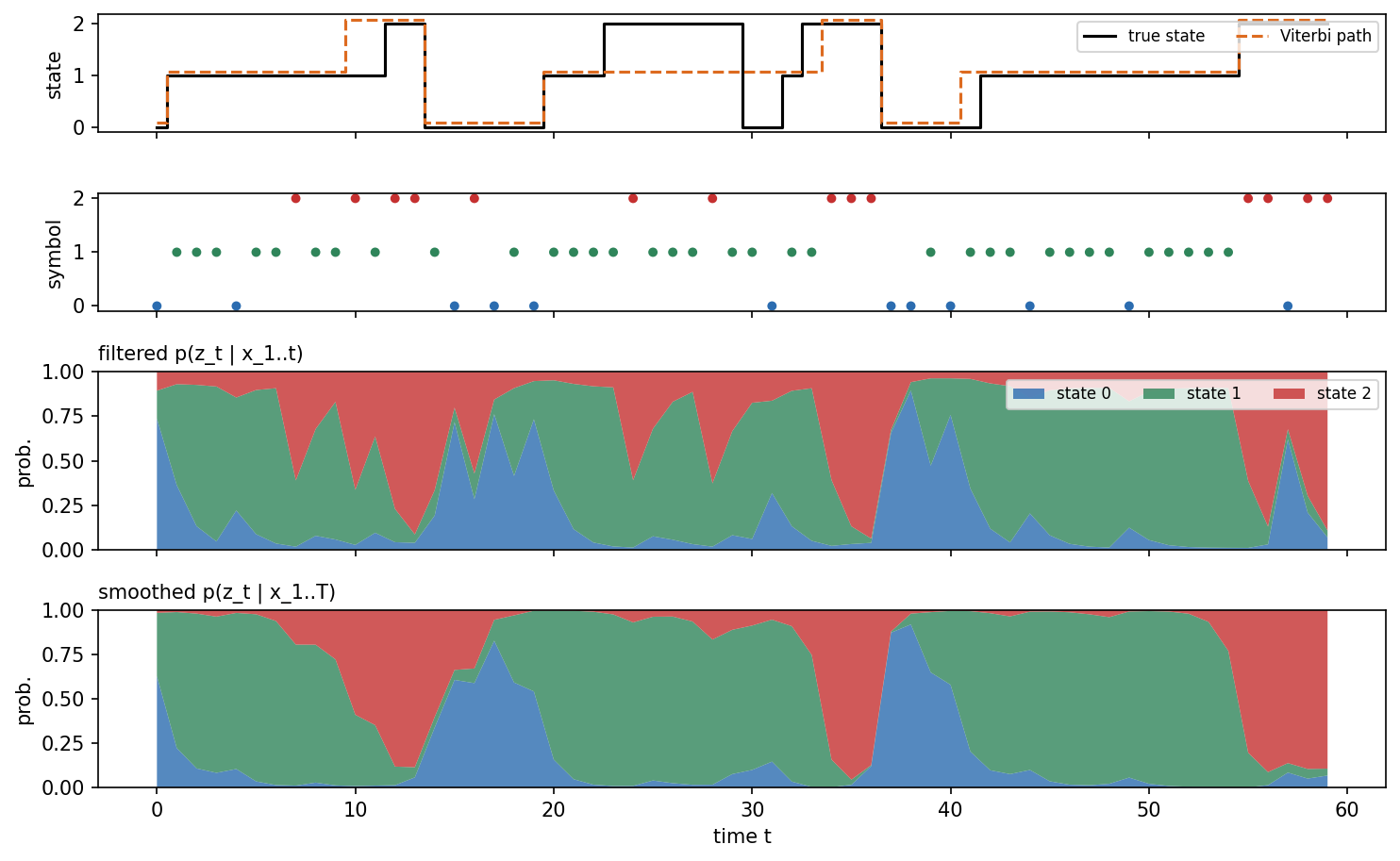
A note on evaluation. If a system must make decisions online, report filtered (or fixed-lag) performance. A smoothed result uses observations that would not yet exist at decision time, and it overstates what the deployed system can do.
Learning: Baum–Welch
When the hidden states are not labeled, the parameters are estimated by expectation–maximization, known for HMMs as the Baum–Welch algorithm [12]. The E-step runs forward–backward to get the expected state occupancies and the expected transitions . The M-step re-estimates
and the emission parameters from observations weighted by (for example, weighted means and covariances for Gaussian emissions). Each iteration does not decrease the likelihood, but the result depends on the initialization and can be a local maximum; PR 07 develops EM in general. If the hidden states are continuous and everything is linear-Gaussian, the same forward recursion becomes the Kalman filter [13]. Neural recurrent models, which replace the discrete state by a learned vector, are covered in ML 04.
Conditional random fields
In plain words. An HMM models how states generate observations, which forces simple assumptions about the observations. When all you need is the labels given the observations, a CRF models that directly, and it can then use any features of the whole input, overlapping or not.
An HMM is generative: it models , including how observations arise. That requires the emission model to describe fully, which is awkward when the features are many, overlapping and dependent (the word itself, its suffix, its capitalization, the neighboring words…). Lafferty, McCallum and Pereira introduced conditional random fields to model the conditional distribution of a label sequence given the observations directly [14]. A linear-chain CRF is
where the are feature functions that may look at the current and previous label and at any part of the input sequence, are learned weights, and normalizes over all label sequences for this particular input [14], [15]. An HMM, written in this form, is a special case in which the features are only “previous label, current label” and “current label, current observation” indicators. The CRF can add arbitrary input features without modeling their distribution.
Inference uses the same dynamic programs as the HMM: the forward algorithm (with log-sum-exp in place of sums) computes and the marginals, and Viterbi finds the best labeling. Training maximizes the conditional log-likelihood , usually with an penalty. For a linear-chain CRF that objective is concave, so there are no bad local optima; its gradient is “observed feature counts minus expected feature counts,” where the expectations come from forward–backward [15]. The code checks the forward computation of against brute force.
Code · Python · 22 lines
import itertools
import numpy as np

rng = np.random.default_rng(0)
T, K = 5, 3
U = rng.normal(size=(T, K))       # unary scores  theta . f(y_t, x, t)
P = rng.normal(size=(K, K))       # transition scores  theta . f(y_{t-1}, y_t)

def score(y):
    return U[np.arange(T), y].sum() + sum(P[y[t - 1], y[t]] for t in range(1, T))

# log Z by the forward recursion in log space (log-sum-exp instead of sum).
log_alpha = U[0].copy()
for t in range(1, T):
    m = log_alpha[:, None] + P
    log_alpha = U[t] + np.logaddexp.reduce(m, axis=0)
log_Z = np.logaddexp.reduce(log_alpha)

brute = np.logaddexp.reduce([score(np.array(y))
                             for y in itertools.product(range(K), repeat=T)])
print("log Z forward:", round(log_Z, 6), " brute force:", round(brute, 6))
assert np.isclose(log_Z, brute)
Both give . Here the scores are random numbers standing in for ; in a real CRF they come from features of , and in modern systems from a neural network.
On images, the same idea gives grid-structured CRFs over pixels, with unary terms from a pixel classifier and pairwise terms like the Potts energy above. Exact inference is no longer possible on loopy grids, so approximate methods are used (PR 08).
Modern view
Templates, alignment, grammars and Markov chains look old-fashioned next to deep networks. In fact each survives, sometimes inside the networks. These are the main threads in the review literature and recent work.
Template matching. Hashemi et al. [4] review the basic concept of matching, advances such as invariant features and deformable models, and applications including medical image analysis. They conclude that template matching works best combined with other recognition steps, for example NCC followed by a robust decision stage. Correlation-based matching is fast, simple and exact when appearance is controlled, and it remains standard in industrial inspection, image registration and as a building block of trackers. When appearance varies, matching moved to learned feature spaces; the “template” is now a feature map, and correlation is computed between deep features, but the operation is the same.
Time-series classification and DTW. Bagnall et al.’s “bake off” [16] reimplemented 18 time-series classification algorithms in one framework and compared them over 100 resamples of each of 85 UCR datasets. Only nine were significantly better than both benchmarks (one of which was 1-NN with DTW), and a collective of transformation-based ensembles (COTE) beat all others. The “bake off redux” by Middlehurst, Schäfer and Bagnall [17] repeated the exercise on the expanded 112-dataset archive plus 30 new problems, added convolution-based, feature-based and deep-learning categories to the taxonomy, and found two recent algorithms, MultiROCKET+Hydra and HIVE-COTE 2, significantly better than the rest. Ismail Fawaz et al. [18] reviewed deep learning for time-series classification with a unified taxonomy and trained 8,730 networks on 97 datasets in one open framework. Meanwhile DTW itself became a building block: soft-DTW [19] replaces the minimum in the DTW recursion by a smooth soft-minimum, which makes it differentiable so it can serve as a loss for training networks and for averaging time series.
Alignment inside neural networks. Connectionist temporal classification (CTC) [20] trains a recurrent network to output label sequences without a frame-by-frame alignment, by summing over all alignments with a forward–backward recursion closely related to the HMM’s. The dynamic program survived; the emission model became a network.
Optional: Connectionist temporal classification (CTC) (in the Supplementary notes). The alignment-summing recursion, the loss, decoding and when its assumptions fail.
CRFs with deep features. Sutton and McCallum’s tutorial [15] remains the standard reference for CRF modeling, inference and training. In vision, fully connected CRFs with Gaussian edge potentials made mean-field inference over all pixel pairs efficient [21] and became a popular refinement step for semantic segmentation; Zheng et al. then wrote that mean-field inference as a recurrent network layer and trained it end to end with the CNN [22]. In language, the BiLSTM-CRF of Lample et al. [23] put a CRF output layer on top of a bidirectional LSTM for named-entity recognition, so that label transitions are modeled explicitly while features are learned. In both areas, later architectures with large receptive fields or attention often model enough context that the explicit CRF adds little, but the structured output layer is still used where label constraints matter.
Structure and graphs. The graph-matching surveys of Conte et al. [8] and Foggia et al. [9] trace the move from exact and error-tolerant matching to graph kernels, graph embeddings and learning-based methods. The modern descendants, graph neural networks, learn node and graph representations by message passing, a direct generalization of the local computations of factor graphs.
State-space models. The idea that a compact hidden state summarizes the past, the core of HMMs and the Kalman filter [13], is central again in sequence modeling. Selective state-space models such as Mamba [24] use input-dependent linear recurrences that run in time linear in the sequence length, offered as an alternative to attention for long sequences.
Open problems. DTW and edit distances are quadratic per comparison, so search over large collections relies on bounds and pruning [6]. Graph edit distance remains expensive to compute exactly. HMM and CRF results depend on the independence assumptions built into the graph; when those are wrong, smoothing can confidently erase short events. And for any online system, the distinction between filtered and smoothed evaluation is easy to get wrong.
Key takeaways
- NCC subtracts means and divides by norms, so it is invariant to brightness offsets and positive contrast changes; SSD and raw correlation are not. Neither handles rotation, scale or deformation.
- DTW finds the cheapest monotone alignment by dynamic programming in ; a Sakoe–Chiba band limits pathological warping and cost, but must be wider than the real timing differences.
- Structural recognition describes patterns as strings, grammars or graphs; edit distance compares strings with the same dynamic-programming pattern as DTW.
- Graphical models factorize joint distributions into local pieces; message passing on chains and trees is exact and efficient.
- HMM algorithms: forward ( and filtering), forward–backward (smoothing), Viterbi (best path), Baum–Welch (learning), all . Scale or work in logs to avoid underflow.
- The Viterbi path and per-step most-probable states answer different questions; the latter can be an impossible sequence.
- CRFs model directly, can use arbitrary overlapping input features, share the HMM’s inference algorithms and have a concave training objective in the linear-chain case.
Exercises
- NCC and negatives. Show that NCC is unchanged when every pixel of a patch is replaced by with . What happens when , and why can NCC not tell you the value of ?
Hint
Subtracting the mean removes entirely, so no information about it survives. The factor appears in the numerator and as in the denominator; it cancels for and flips the sign for (a photographic negative of a perfect match scores ).
- DTW by hand. Compute the DTW distance with cost between and . Write out the table and the optimal path. What is the lock-step distance, and why is it not even defined here?
Hint
The optimal path matches to both zeros, then and , with total cost 0. Lock-step comparison needs equal lengths, which these sequences do not have; DTW handles unequal lengths naturally.
- A forbidden transition. Construct your own two- or three-state HMM with one transition probability set to zero and an observation sequence for which the per-step argmax of is an impossible state sequence. Verify with the code above.
Hint
You need two neighboring time steps whose individually most likely states are joined by the forbidden transition. A symmetric or cyclic model with ambiguous emissions (probabilities close to 0.5) makes this easy; then check that joint(marginal) is 0.
- Online versus offline. An activity recognizer reports 95% accuracy computed from smoothed state probabilities on recorded sequences. It will run on a phone and must decide at each second. What information advantage does the reported number include, and what would you report instead?
Hint
Smoothing uses observations from the future of each decision. Report filtered accuracy, or fixed-lag smoothing with the lag the application can tolerate (for example decisions delayed by 2 seconds use observations up to ).
- From HMM to CRF. Write an HMM’s as a sum of feature functions times weights, in the form of the linear-chain CRF. Which features and weights do you get? What extra features could a CRF add for part-of-speech tagging that an HMM cannot easily use?
Hint
Use indicator features with weight , with weight , and with weight . A CRF can add features such as “the next word ends in -ly” or “the current word is capitalized,” which overlap with and depend on the word identity.
- Edit distance with weights. Modify
edit_distanceso that substituting two directions that differ by 90 degrees costs 1 and by 180 degrees costs 2. Recompute the distances in the chain-code example. Does the ranking change?
Hint
The substitution cost is the circular difference between direction codes. The bumped square needs only insertions, so its distance stays 2; check whether the rectangle’s distance changes, given which substitutions its cheapest edit sequence uses.
References
- S. Theodoridis and K. Koutroumbas, Pattern Recognition, 4th ed., Academic Press, 2009, Chapters 8 and 9. publisher page
- C. M. Bishop, Pattern Recognition and Machine Learning, Springer, 2006, Sections 8.1–8.4 and 13.1–13.3. official book page and PDF
- J. P. Lewis, “Fast Normalized Cross-Correlation,” Vision Interface, 1995. paper
- N. S. Hashemi, R. B. Aghdam, A. S. B. Ghiasi, and P. Fatemi, “Template Matching Advances and Applications in Image Analysis,” arXiv:1610.07231, 2016. arXiv
- H. Sakoe and S. Chiba, “Dynamic Programming Algorithm Optimization for Spoken Word Recognition,” IEEE Transactions on Acoustics, Speech, and Signal Processing, vol. 26, no. 1, pp. 43–49, 1978. doi:10.1109/TASSP.1978.1163055
- T. Rakthanmanon, B. Campana, A. Mueen, G. Batista, B. Westover, Q. Zhu, J. Zakaria, and E. Keogh, “Searching and Mining Trillions of Time Series Subsequences under Dynamic Time Warping,” Proceedings of the 18th ACM SIGKDD International Conference on Knowledge Discovery and Data Mining, pp. 262–270, 2012. doi:10.1145/2339530.2339576
- R. A. Wagner and M. J. Fischer, “The String-to-String Correction Problem,” Journal of the ACM, vol. 21, no. 1, pp. 168–173, 1974. doi:10.1145/321796.321811
- D. Conte, P. Foggia, C. Sansone, and M. Vento, “Thirty Years of Graph Matching in Pattern Recognition,” International Journal of Pattern Recognition and Artificial Intelligence, vol. 18, no. 3, pp. 265–298, 2004. doi:10.1142/S0218001404003228
- P. Foggia, G. Percannella, and M. Vento, “Graph Matching and Learning in Pattern Recognition in the Last 10 Years,” International Journal of Pattern Recognition and Artificial Intelligence, vol. 28, no. 1, 1450001, 2014. doi:10.1142/S0218001414500013
- L. R. Rabiner, “A Tutorial on Hidden Markov Models and Selected Applications in Speech Recognition,” Proceedings of the IEEE, vol. 77, no. 2, pp. 257–286, 1989. doi:10.1109/5.18626
- A. J. Viterbi, “Error Bounds for Convolutional Codes and an Asymptotically Optimum Decoding Algorithm,” IEEE Transactions on Information Theory, vol. 13, no. 2, pp. 260–269, 1967. doi:10.1109/TIT.1967.1054010
- L. E. Baum, T. Petrie, G. Soules, and N. Weiss, “A Maximization Technique Occurring in the Statistical Analysis of Probabilistic Functions of Markov Chains,” The Annals of Mathematical Statistics, vol. 41, no. 1, pp. 164–171, 1970. doi:10.1214/aoms/1177697196
- R. E. Kalman, “A New Approach to Linear Filtering and Prediction Problems,” Journal of Basic Engineering, vol. 82, no. 1, pp. 35–45, 1960. doi:10.1115/1.3662552
- J. D. Lafferty, A. McCallum, and F. C. N. Pereira, “Conditional Random Fields: Probabilistic Models for Segmenting and Labeling Sequence Data,” Proceedings of the 18th International Conference on Machine Learning (ICML), pp. 282–289, 2001. paper page
- C. Sutton and A. McCallum, “An Introduction to Conditional Random Fields,” Foundations and Trends in Machine Learning, vol. 4, no. 4, pp. 267–373, 2012. doi:10.1561/2200000013
- A. Bagnall, J. Lines, A. Bostrom, J. Large, and E. Keogh, “The Great Time Series Classification Bake Off: A Review and Experimental Evaluation of Recent Algorithmic Advances,” Data Mining and Knowledge Discovery, vol. 31, pp. 606–660, 2017. doi:10.1007/s10618-016-0483-9
- M. Middlehurst, P. Schäfer, and A. Bagnall, “Bake Off Redux: A Review and Experimental Evaluation of Recent Time Series Classification Algorithms,” Data Mining and Knowledge Discovery, vol. 38, pp. 1958–2031, 2024. doi:10.1007/s10618-024-01022-1
- H. Ismail Fawaz, G. Forestier, J. Weber, L. Idoumghar, and P.-A. Muller, “Deep Learning for Time Series Classification: A Review,” Data Mining and Knowledge Discovery, vol. 33, pp. 917–963, 2019. doi:10.1007/s10618-019-00619-1
- M. Cuturi and M. Blondel, “Soft-DTW: A Differentiable Loss Function for Time-Series,” ICML, 2017. arXiv:1703.01541
- A. Graves, S. Fernández, F. Gomez, and J. Schmidhuber, “Connectionist Temporal Classification: Labelling Unsegmented Sequence Data with Recurrent Neural Networks,” Proceedings of the 23rd International Conference on Machine Learning (ICML), pp. 369–376, 2006. doi:10.1145/1143844.1143891
- P. Krähenbühl and V. Koltun, “Efficient Inference in Fully Connected CRFs with Gaussian Edge Potentials,” NIPS, 2011. arXiv:1210.5644
- S. Zheng, S. Jayasumana, B. Romera-Paredes, V. Vineet, Z. Su, D. Du, C. Huang, and P. H. S. Torr, “Conditional Random Fields as Recurrent Neural Networks,” ICCV, 2015. arXiv:1502.03240
- G. Lample, M. Ballesteros, S. Subramanian, K. Kawakami, and C. Dyer, “Neural Architectures for Named Entity Recognition,” NAACL, 2016. arXiv:1603.01360
- A. Gu and T. Dao, “Mamba: Linear-Time Sequence Modeling with Selective State Spaces,” arXiv:2312.00752, 2023. arXiv
Check your understanding
This tutorial has 6 exercises. Can you solve them without opening the hints?
Go to the exercises ↑Next PR 07 · Clustering, Mixtures and EM · 26 min