PR 09 · Ensembles, Validation and Cluster Validity
Needs: PR 08 · Approximate Inference and Bayesian Model Complexity
Navigate: this page and this track: Navigate: this page and this track
On this page
- What you’ll learn1 min
- The big picture1 min
- Bias, variance and noise3 min
- Trees and partitions1 min
- Bagging and random forests2 min
- Boosting changes the next learner’s job4 min
- Averaging is not always the same operation2 min
- Validation estimates a procedure5 min
- Comparing classifiers statistically3 min
- Measure decisions and probabilities1 min
- Cluster validity as model selection1 min
- Modern view2 min
- Key takeaways1 min
- Exercises3 min
- Paper guides
- References
Pattern Recognition
Explore this chapter 1 interactive experiment
Grow real decision trees on 300 noisy two-moons points, bootstrap them, let them vote, and watch the test error fall and then flatten as trees are added.
What you’ll learn
- Derive the bias–variance decomposition of squared error and use it to explain why averaging helps unstable learners.
- Explain how decision trees partition feature space, and how bagging and random forests reduce their variance, including out-of-bag estimates.
- Derive AdaBoost from exponential loss, connect it to gradient boosting, and distinguish boosting, voting, Bayesian model averaging and stacking.
- Estimate the performance of a whole recognition procedure with hold-out, k-fold, group-aware and nested cross-validation and with the bootstrap (.632 and .632+).
- Compare two or more classifiers with McNemar’s test, the 5×2cv and corrected resampled t-tests, and the Friedman/Nemenyi procedure, and know when each is valid.
- Evaluate probabilities as well as decisions, and treat cluster validity as a model-selection question.
The big picture
A single recognizer makes mistakes for two very different reasons. Sometimes it is too simple to express the true decision rule; sometimes it is so flexible that it memorizes accidents of the particular training set. Ensembles attack the second problem (bagging, random forests) or the first (boosting) by combining many models. Validation is the other half of the story: once we can build many models and tune many knobs, we need a trustworthy way to estimate how the chosen procedure will perform on new data, and to decide whether one procedure is really better than another.
Why it matters: tree ensembles remain among the strongest methods for tabular features, including hand-crafted image descriptors [23], deep-network ensembles are a standard way to obtain uncertainty estimates [24], and almost every published comparison between recognizers rests on cross-validation and a statistical test. Theodoridis and Koutroumbas treat decision trees, classifier combination and boosting in Chapter 4, error estimation and comparison in Chapter 10 (“Supervised Learning: The Epilogue”), and cluster validity in Chapter 16 [1]. Bishop’s Chapter 14 separates several mathematically different ways to combine models, and Section 3.2 derives the bias–variance decomposition [2]. Classifiers themselves were covered in PR 03 and PR 04.
Bias, variance and noise
Plain version. Imagine retraining the same learning algorithm on many different training sets drawn from the same source. The average prediction may still miss the truth: that systematic miss is bias. The individual predictions scatter around their average: that scatter is variance. Even a perfect predictor cannot remove the randomness in the labels themselves: that is noise.
Precise version. Let the target be , where is the unknown regression function and is noise with and , independent of everything else. A learning algorithm maps a random training set to a predictor . Write for the average prediction over training sets. At a fixed input , the expected squared error over training sets and test noise is
The three cross terms vanish: has zero mean and is independent of , is a constant, and by the definition of . Averaging over the input distribution gives the expected test error. Geman, Bienenstock and Doursat named the resulting tension the bias/variance dilemma [3]: making a model more flexible typically lowers bias and raises variance, and the best complexity balances the two.
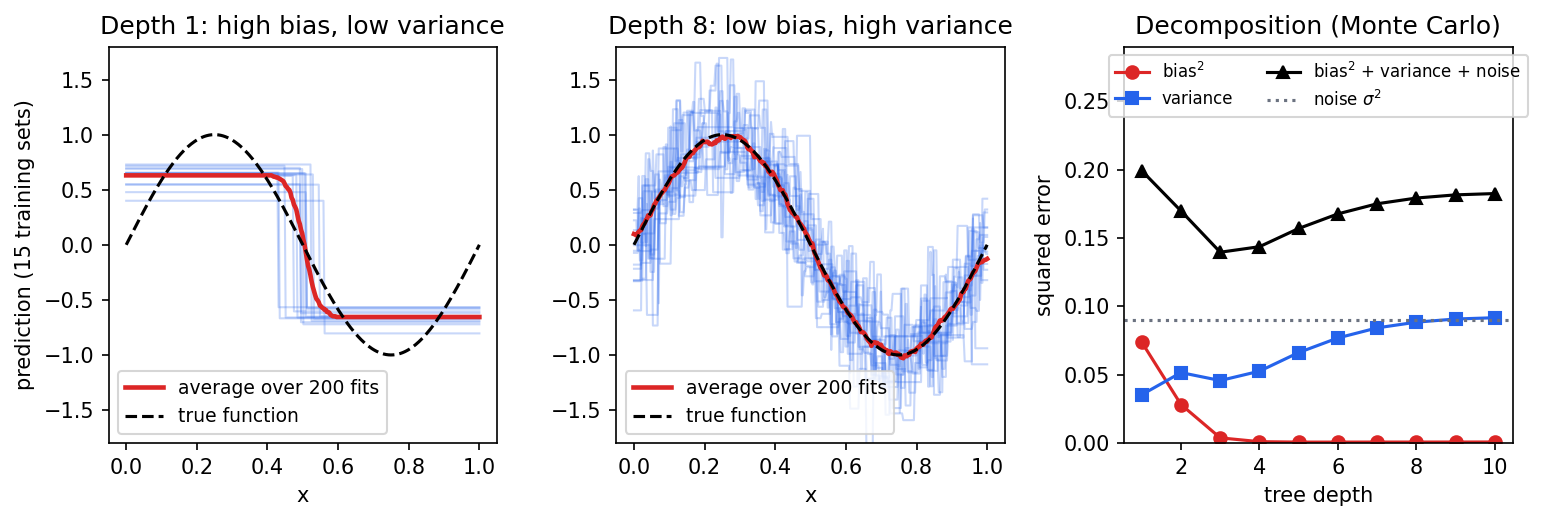
The code below estimates each term by brute force for regression trees of growing depth on a noisy sine curve. Two hundred training sets of 60 points each are drawn; the empirical average and spread of the 200 fitted trees give bias² and variance.
Code · Python · 24 lines
import numpy as np
from sklearn.tree import DecisionTreeRegressor

rng = np.random.default_rng(0)
f = lambda x: np.sin(2 * np.pi * x)          # true regression function
sigma = 0.3                                   # noise standard deviation
x_test = np.linspace(0, 1, 200)[:, None]

def bias_variance(depth, n_sets=200, n=60):
    preds = np.empty((n_sets, len(x_test)))
    for s in range(n_sets):                   # many independent training sets
        x = rng.random((n, 1))
        y = f(x[:, 0]) + rng.normal(0, sigma, n)
        tree = DecisionTreeRegressor(max_depth=depth, random_state=0)
        preds[s] = tree.fit(x, y).predict(x_test)
    mean_pred = preds.mean(axis=0)
    bias2 = np.mean((mean_pred - f(x_test[:, 0])) ** 2)
    var = np.mean(preds.var(axis=0))
    return bias2, var

for depth in [1, 2, 3, 5, 8, None]:
    b2, v = bias_variance(depth)
    print(f"depth={str(depth):>4}  bias^2={b2:.4f}  variance={v:.4f}  "
          f"expected test MSE~{b2 + v + sigma**2:.4f}")
On our run, depth 1 gives bias² ≈ 0.074 and variance ≈ 0.035, depth 3 gives the lowest total (bias² ≈ 0.003, variance ≈ 0.045), and fully grown trees have almost no bias but variance ≈ 0.092, as large as the noise variance itself. Figure 1 shows the same experiment visually.
Three cautions keep the picture honest. First, the clean decomposition is specific to squared error; for 0–1 classification loss there are several competing definitions and bias and variance can interact non-additively, so use the decomposition as intuition rather than as an exact accounting for classifiers. Second, “complexity” is not just parameter count: depth, regularization strength, number of boosting rounds and early stopping all move a model along the bias–variance axis. Third, very large over-parameterized models can show a test-error curve that rises and then falls again as capacity grows past the interpolation point, the “double descent” shape documented by Belkin and colleagues [25]. The decomposition still holds pointwise; what changes is how variance behaves as capacity grows.
Optional: Double descent: reading Belkin, Hsu, Ma and Mandal (PNAS 2019) (in the Paper guides). A reading guide to what the curves plot and how they were produced, with a small minimum-norm experiment you can run.
Trees and partitions
Plain version. A decision tree asks a sequence of yes/no questions about the features, such as “is feature 3 below 0.7?”, and each final answer box (a leaf) stores a prediction. It is the classical example of a low-bias, high-variance learner, which is exactly why it is the favorite building block for ensembles.
Precise version. A tree recursively divides observations by conditions such as . Each leaf estimates a class distribution (classification) or a constant (regression). For a classification node with class proportions , the Gini impurity is
and the entropy is . Both are zero for a pure node and largest for a uniform mix. A split of a parent node into children and , holding and of its samples, is scored by the impurity decrease
and the learner chooses the feature and threshold with the largest . This is a greedy local choice: the best single split need not lead to the best tree. A deep tree can capture interactions and nonlinear, axis-aligned boundaries, but it can change substantially when a few training points change; that instability is exactly the high variance seen in Figure 1.
Depth limits, minimum leaf sizes and cost-complexity pruning constrain complexity. Because splits depend only on the ordering of each feature, trees are invariant to monotone rescaling, which makes scaling less critical than for distance-based models; missing values, feature definitions and train-only transformations still require care. Theodoridis and Koutroumbas (Chapter 4) and Bishop (Section 14.4) treat trees as one family of nonlinear classifiers [1], [2].
Bagging and random forests
Plain version. Bagging (“bootstrap aggregating”) builds many training sets by sampling the original data with replacement, trains one unstable model on each, and averages or votes. Random forests add one more source of randomness, a random subset of features at every split, so that the trees disagree more and their average improves more.
Precise version. Breiman introduced bagging as a way to improve unstable procedures, those whose output changes a lot under small perturbations of the training set [4]. Given bootstrap samples , each of size , the bagged regressor is and the bagged classifier takes a majority vote (or averages class probabilities).
Why does averaging help? Suppose scalar predictors at a fixed each have variance and every pair has correlation . Expanding the variance of a sum,
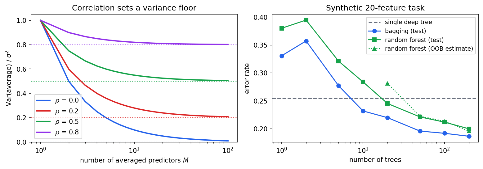
The second term vanishes as grows, but the first term does not: correlated errors set a floor (Figure 2, left). Averaging leaves the bias essentially unchanged, so bagging helps most for low-bias, high-variance learners such as deep trees, and little for stable learners such as linear discriminants or -nearest neighbors with large . This illustrative formula explains why correlated errors limit gains; it does not promise that every classification ensemble improves accuracy.
Random forests reduce directly [5]. When growing each tree on its bootstrap sample, every split considers only a random subset of features (a common default for classification is of features). Breiman showed that the forest’s generalization error is bounded in terms of the strength of the individual trees and the correlation between them [5], which is the same trade-off as the variance formula: weaker but less correlated trees can make a stronger forest.
Out-of-bag (OOB) estimates. The probability that a given observation is not drawn in draws with replacement is . Each tree therefore leaves out about 37% of the data, and each observation can be predicted by the roughly one third of trees that never saw it. Aggregating those predictions gives an OOB error estimate essentially for free [5]. In Figure 2 (right) the OOB estimate tracks the test error once there are enough trees. But ordinary bootstrapping resamples rows: if several rows share a subject, writer or recording, a tree can train on one image of a person and be “tested” OOB on another image of the same person. The OOB score is then optimistic for deployment to new groups.
Boosting changes the next learner’s job
Plain version. Bagging trains its members independently and in parallel. Boosting trains them in sequence: each new weak learner concentrates on the examples the current ensemble still gets wrong, and the final prediction is a weighted sum. Bagging mainly reduces variance; boosting mainly reduces bias, turning many “slightly better than chance” rules into a strong classifier.
Precise version. Boosting builds an additive model
where each is a weak learner (often a depth-1 tree, a stump) and its weight. The class prediction for labels is .
The AdaBoost algorithm
Freund and Schapire’s AdaBoost [6] works as follows, for training pairs , :
- Start with uniform weights .
- For :
- fit to the training data using weights ;
- compute the weighted error ;
- set ;
- update and renormalize.
- Output .
Misclassified points have , so their weight is multiplied by ; correctly classified points are multiplied by . A learner with gets a positive vote, and the better it is, the larger the vote.
Deriving AdaBoost from exponential loss
Friedman, Hastie and Tibshirani showed that AdaBoost is forward stagewise additive modeling with the exponential loss [7]. Suppose is fixed and we add one term . The training loss is
The weights do not depend on or . Split the sum into correctly and incorrectly classified points:
Step 1, choose . For any , the first coefficient is positive, so the best minimizes the weighted training error: exactly “fit with weights .”
Step 2, choose . Divide by and write for the normalized weighted error. We minimize . Setting gives , that is,
Step 3, update weights. The next weights are , the AdaBoost update. Every step of the algorithm is thus recovered from greedy minimization of exponential loss.
Two consequences follow. Since , the training error is bounded by the average exponential loss; with the optimal , each round multiplies that bound by whenever , so training error falls exponentially fast if every weak learner beats chance by a margin [6]. And the minimizer of expected exponential loss is , half the log-odds [7], so is a (not necessarily well-calibrated) probability estimate. The exponential weight also explains a known weakness: a mislabeled point receives exponentially growing weight, so AdaBoost can be sensitive to label noise and outliers.
The code implements AdaBoost from scratch with weighted stumps and checks it against scikit-learn’s AdaBoostClassifier. For two classes scikit-learn’s SAMME variant uses , twice ours, which rescales but leaves every sign, and every renormalized weight, unchanged.
Code · Python · 42 lines
import numpy as np
from sklearn.datasets import make_classification
from sklearn.model_selection import train_test_split
from sklearn.tree import DecisionTreeClassifier
from sklearn.ensemble import AdaBoostClassifier

X, y01 = make_classification(n_samples=600, n_features=10, n_informative=4,
                             flip_y=0.05, random_state=1)
y = 2 * y01 - 1                                   # labels in {-1, +1}
Xtr, Xte, ytr, yte = train_test_split(X, y, test_size=0.3, random_state=1)

def adaboost_fit(X, y, M=100):
    n = len(y)
    w = np.full(n, 1 / n)                         # step 1: uniform weights
    stumps, alphas = [], []
    for m in range(M):
        h = DecisionTreeClassifier(max_depth=1, random_state=0)
        h.fit(X, y, sample_weight=w)              # step 2a: weighted fit
        pred = h.predict(X)
        err = np.sum(w * (pred != y)) / np.sum(w) # step 2b: weighted error
        err = np.clip(err, 1e-12, 1 - 1e-12)
        alpha = 0.5 * np.log((1 - err) / err)     # step 2c: learner weight
        w = w * np.exp(-alpha * y * pred)         # step 2d: reweight
        w /= w.sum()
        stumps.append(h); alphas.append(alpha)
    return stumps, np.array(alphas)

def adaboost_score(stumps, alphas, X):
    return sum(a * h.predict(X) for h, a in zip(stumps, alphas))

stumps, alphas = adaboost_fit(Xtr, ytr)
F_tr = adaboost_score(stumps, alphas, Xtr)
F_te = adaboost_score(stumps, alphas, Xte)
print("from scratch: train err", np.mean(np.sign(F_tr) != ytr),
      " test err", np.mean(np.sign(F_te) != yte))
print("exp-loss bound on train err:", np.mean(np.exp(-ytr * F_tr)))

ref = AdaBoostClassifier(DecisionTreeClassifier(max_depth=1, random_state=0),
                         n_estimators=100, random_state=0).fit(Xtr, ytr)
agree = np.mean(ref.predict(Xte) == np.sign(F_te))
print("sklearn test err", np.mean(ref.predict(Xte) != yte),
      " agreement with ours:", agree)
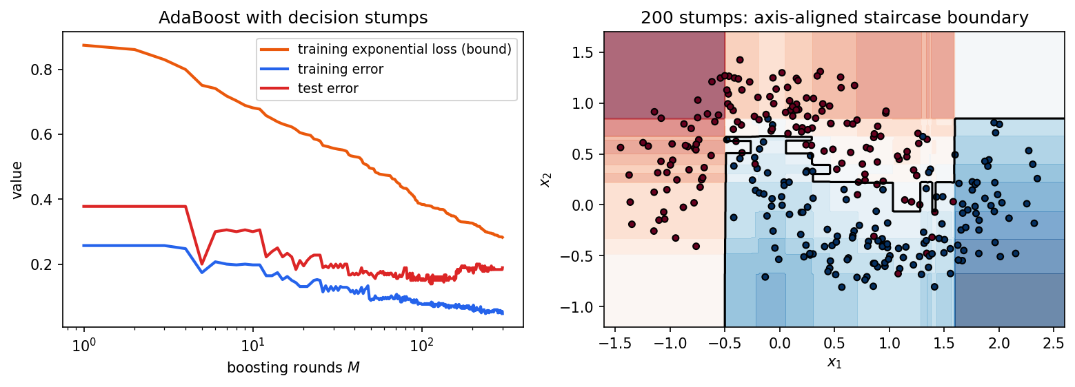
With scikit-learn 1.6 our run prints a training error of 0.076, an exponential-loss bound of 0.384, a test error of 0.156 for both implementations and 100% agreement on test predictions. Figure 3 shows the curves over 300 rounds and the staircase boundary that stumps build in two dimensions.
Gradient boosting
Plain version. Gradient boosting generalizes the AdaBoost idea to any differentiable loss: at each round, compute in which direction each training prediction should move to reduce the loss, and fit a small tree to those directions.
Precise version. Friedman’s gradient boosting machine [8] performs gradient descent in function space. At round , compute the pseudo-residuals
fit a regression tree to the pairs by least squares, choose a step by line search (or one optimal constant per leaf, Friedman’s TreeBoost), and update with a learning rate (shrinkage) . For squared error the pseudo-residual is the ordinary residual . For binary log loss with and the log-odds, it is : the label minus the predicted probability, not minus the predicted class. With exponential loss and a line search, the procedure reduces to a version of AdaBoost.
The learning rate, the number of rounds and the tree size interact: a smaller needs more rounds but usually generalizes better, and the number of rounds is chosen by early stopping on validation data, never on the final test. XGBoost [9] made gradient-boosted trees fast and scalable through a regularized objective, second-order (Newton) leaf values, sparsity-aware split finding and a weighted quantile sketch; histogram-based implementations such as scikit-learn’s HistGradientBoostingClassifier follow the same principles [26].
Averaging is not always the same operation
Many methods “combine models,” but they answer different questions.
| Method | What supplies the combination? | Main caution |
|---|---|---|
| Voting or probability averaging (bagging, forests) | fixed equal combination of independently trained predictors | correlated errors and incompatible calibration |
| Boosting | sequential fitting; weights from a loss | label noise; needs early stopping |
| Bayesian model averaging | posterior probability over model hypotheses | evidence and priors must be meaningful |
| Stacking | a learned predictor of base-model outputs | train it on out-of-fold predictions |
| Conditional mixtures (mixtures of experts) | input-dependent gates or responsibilities | experts and gate can overfit together |
Bayesian model averaging (Bishop Section 14.1 [2]) uses
where is the posterior probability of model . Those weights are posterior model probabilities, not arbitrary validation accuracies, and with plenty of data they tend to concentrate on one model. BMA expresses uncertainty about which model generated the data; a committee or ensemble instead builds a richer model out of several parts [2]. The model evidence connects to the approximate-inference tools of PR 08.
Stacking (stacked generalization, Wolpert [10]) instead learns a mapping from base-model predictions to the target. Its training features must come from base models that did not train on those same examples; otherwise the stacker learns from unrealistically easy, overfitted predictions. The standard recipe: split the training set into folds, fit each base model on folds and predict the held-out fold, collect these out-of-fold predictions as features, fit a simple meta-learner (often regularized logistic regression) on them, and finally refit the base models on all training data.
The following comparison on scikit-learn’s bundled breast-cancer dataset (569 samples, 30 features) runs every method inside the same stratified 5-fold cross-validation, so all numbers are comparable. StackingClassifier builds its own inner out-of-fold predictions (cv=5) inside each outer training fold.
Code · Python · 30 lines
import numpy as np
from sklearn.datasets import load_breast_cancer
from sklearn.model_selection import StratifiedKFold, cross_val_score
from sklearn.pipeline import make_pipeline
from sklearn.preprocessing import StandardScaler
from sklearn.linear_model import LogisticRegression
from sklearn.tree import DecisionTreeClassifier
from sklearn.ensemble import (BaggingClassifier, RandomForestClassifier,
                              HistGradientBoostingClassifier, StackingClassifier)

X, y = load_breast_cancer(return_X_y=True)
cv = StratifiedKFold(n_splits=5, shuffle=True, random_state=0)
logreg = make_pipeline(StandardScaler(), LogisticRegression(max_iter=2000))
models = {
    "single tree": DecisionTreeClassifier(random_state=0),
    "bagged trees": BaggingClassifier(DecisionTreeClassifier(), n_estimators=100,
                                      random_state=0),
    "random forest": RandomForestClassifier(n_estimators=100, random_state=0),
    "hist. gradient boosting": HistGradientBoostingClassifier(random_state=0),
    "logistic regression": logreg,
}
models["stacking"] = StackingClassifier(
    estimators=[("rf", models["random forest"]),
                ("gb", models["hist. gradient boosting"]),
                ("lr", logreg)],
    final_estimator=LogisticRegression(max_iter=2000),
    cv=5, stack_method="predict_proba")
for name, model in models.items():
    s = cross_val_score(model, X, y, cv=cv, scoring="accuracy")
    print(f"{name:>24}: {s.mean():.3f} +/- {s.std():.3f}")
Our run gives mean accuracies of 0.926 (single tree), 0.960 (bagging), 0.965 (forest), 0.970 (gradient boosting), 0.979 (logistic regression) and 0.979 (stacking), with fold standard deviations between 0.009 and 0.022. Two lessons follow. Ensembling clearly fixes the unstable single tree. But a well-regularized linear model is already as good as the stack on this small, nearly linearly separable dataset, and the differences among the top four are within one fold standard deviation. Whether any of them is significantly better is a question for the statistical tests later in this chapter, not for eyeballing means.
Validation estimates a procedure
Plain version. A test score is only trustworthy if the test data played no part in building the model. Every choice we make while looking at data, including features, hyperparameters, thresholds, and even which algorithm to use, is part of the “model,” and must be made without the data used to judge it.
Training fits parameters. Validation selects hyperparameters, features, thresholds and calibration choices. Testing assesses the selected procedure. Every adaptive choice consumes information from whichever data it examines. Strictly speaking, cross-validation estimates the performance of a procedure (an algorithm plus its tuning rules) trained on data sets of a given size, rather than the error of the one fitted model you will ship; Bates, Hastie and Tibshirani make this precise and show that naive cross-validation confidence intervals can undercover [19].
Hold-out, k-fold and leave-one-out
- Hold-out. Split once into training and test parts. Simple and cheap, but with small data the estimate has high variance and depends on the split, and the model is trained on less data than you have.
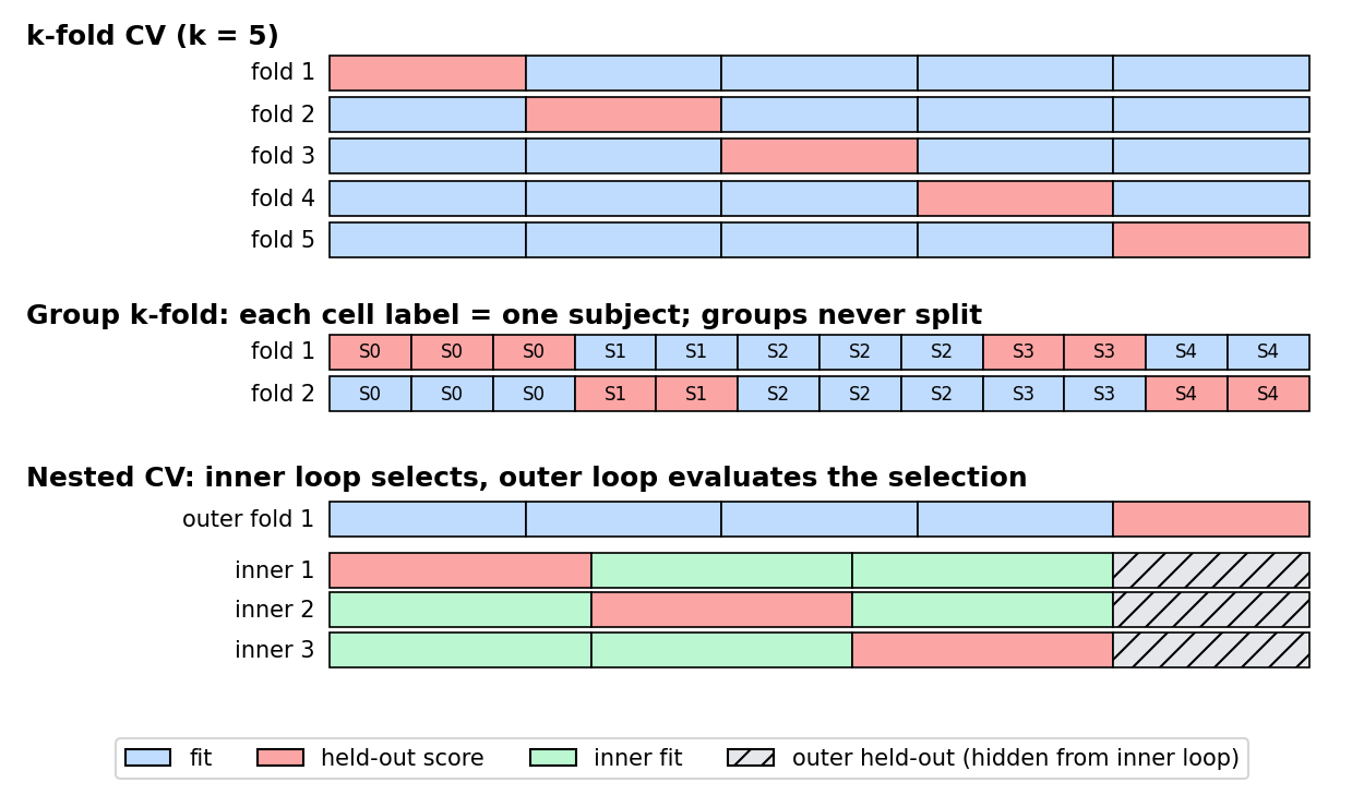
- k-fold cross-validation. Partition the data into folds; train on and score the remaining one, rotating so each fold is held out once (Figure 4, top). The CV estimate is , where is the fold containing sample and is the model trained without fold . Values or are common compromises: each model sees 80–90% of the data, so the pessimistic bias is small, and the cost is fits.
- Leave-one-out (LOO). The case . Nearly unbiased for the size- procedure, but it requires fits (unless a closed form exists, as for linear smoothers or -NN) and can have high variance because the training sets are almost identical.
- Stratification keeps class proportions similar across folds, which matters for rare classes. It does not fix dependence between samples.
Arlot and Celisse survey the theory of these choices for both estimating risk and selecting models [18].
Groups and time
For observations sharing a patient, writer, camera or recording session, hold whole groups together (Figure 4, middle). Otherwise near-duplicate images of the same person land on both sides of the split and the score measures memorization of that person, not recognition of new people. Time-ordered data needs chronological splits (train on the past, test on the future). The rule is to make the split mirror the deployment question: “new images of known writers” and “images of new writers” are different questions and deserve different splits.
The bootstrap, .632 and .632+
Plain version. Instead of folds, draw many bootstrap samples, train on each, and test on the points each one left out.
Precise version. Draw bootstrap samples of size with replacement. For each, fit the model and evaluate it on the out-of-bootstrap points (about 36.8% of the data). The average is the leave-one-out bootstrap error . Because each bootstrap model is trained on only about 63.2% of distinct points, is pessimistic, while the resubstitution (training) error is optimistic. Efron’s .632 estimator blends them:
It fails for heavily overfitting learners such as 1-nearest neighbor, whose training error is zero. Efron and Tibshirani’s .632+ estimator [11] fixes this by moving weight toward as overfitting grows. Let be the no-information error rate (the error if inputs and labels were independent: , with the observed proportion of class and the proportion of predictions equal to ), and define the relative overfitting rate , clipped to . Then
When (no overfitting) it reduces to .632; when it becomes .
Code · Python · 31 lines
import numpy as np
from sklearn.datasets import make_classification
from sklearn.neighbors import KNeighborsClassifier
from sklearn.model_selection import cross_val_score, KFold

X, y = make_classification(n_samples=200, n_features=6, n_informative=3,
                           flip_y=0.1, random_state=3)
model = KNeighborsClassifier(n_neighbors=1)          # resubstitution error is 0
rng = np.random.default_rng(3)
n, B = len(y), 200
resub = np.mean(model.fit(X, y).predict(X) != y)
oob_errs = []
for b in range(B):
    idx = rng.integers(0, n, n)                       # draw n with replacement
    out = np.setdiff1d(np.arange(n), idx)             # ~36.8% left out
    model.fit(X[idx], y[idx])
    oob_errs.append(np.mean(model.predict(X[out]) != y[out]))
err_boot1 = np.mean(oob_errs)                          # leave-one-out bootstrap
err_632 = 0.368 * resub + 0.632 * err_boot1
cv10 = 1 - cross_val_score(model, X, y,
                           cv=KFold(10, shuffle=True, random_state=3)).mean()
print(f"resubstitution {resub:.3f}  OOB bootstrap {err_boot1:.3f}  "
      f".632 {err_632:.3f}  10-fold CV {cv10:.3f}")

# .632+ : shrink toward the out-of-bootstrap error when overfitting is large.
pred = model.fit(X, y).predict(X)
gamma = sum(np.mean(y == k) * (1 - np.mean(pred == k)) for k in np.unique(y))
R = np.clip((err_boot1 - resub) / (gamma - resub), 0, 1)
w = 0.632 / (1 - 0.368 * R)
print(f"no-information rate {gamma:.3f}  R {R:.3f}  "
      f".632+ {(1 - w) * resub + w * err_boot1:.3f}")
For 1-NN the resubstitution error is 0.000, the out-of-bootstrap error 0.332, the .632 estimate only 0.210 (pulled down by the meaningless zero), the .632+ estimate 0.278 and 10-fold CV 0.325. The .632 estimator is badly optimistic here; .632+ repairs most of the gap. In practice, 10-fold CV (possibly repeated) and .632+ are both reasonable; the bootstrap is attractive for very small samples and for confidence intervals.
Nested cross-validation
Plain version. If you tune hyperparameters by cross-validation and then report that same cross-validation score, you report the score of the luckiest configuration, which is optimistic. Nested CV puts the whole tuning process inside an outer loop.
Nested cross-validation has an inner loop for selection and an outer loop for evaluating that selection procedure (Figure 4, bottom). Within each outer training set, an inner CV chooses hyperparameters; the chosen configuration is refit on the whole outer training set and scored on the outer held-out fold, which the inner loop never saw. Varma and Simon showed that reporting the inner (tuning) CV score can be substantially biased, and that nested CV gives nearly unbiased estimates [12]. Cawley and Talbot went further: overfitting the model-selection criterion itself can cost as much as the differences between learning algorithms, so a low-variance selection criterion matters as much as an unbiased one [13]. Refit preprocessing (scaling, feature selection, PCA) inside each inner fold, typically by placing it in a Pipeline. Report variability across outer folds, but do not treat correlated fold scores as independent measurements for a naive confidence interval.
After estimating the procedure, select on development data and evaluate once on an untouched test. Repeatedly inspecting test errors and redesigning the model turns that test into another validation set.
Code: nested selection without group leakage
This CPU example creates three noisy repeated measurements of each synthetic subject. Group labels describe subjects, not classes. The outer loop estimates the selected forest procedure; a separate group-disjoint test set remains untouched until final reporting.
Code · Python · 39 lines
import numpy as np
from sklearn.datasets import make_classification
from sklearn.ensemble import RandomForestClassifier
from sklearn.model_selection import train_test_split, GroupKFold, GridSearchCV
from sklearn.metrics import balanced_accuracy_score, log_loss

rng = np.random.default_rng(9)
subject_x, subject_y = make_classification(
    n_samples=180, n_features=8, n_informative=5, n_redundant=1,
    class_sep=1.0, random_state=9)
groups = np.repeat(np.arange(180), 3)
X = subject_x[groups] + rng.normal(0, 0.03, (len(groups), 8))
y = subject_y[groups]
dev_groups, test_groups = train_test_split(
    np.arange(180), test_size=0.25, stratify=subject_y, random_state=9)
dev = np.flatnonzero(np.isin(groups, dev_groups))
test = np.flatnonzero(np.isin(groups, test_groups))
assert not set(groups[dev]) & set(groups[test])

def search():
    return GridSearchCV(
        RandomForestClassifier(n_estimators=60, random_state=9, n_jobs=1),
        {"max_depth": [3, None], "min_samples_leaf": [1, 3]},
        cv=GroupKFold(3), scoring="balanced_accuracy")

outer_scores = []
for fit, valid in GroupKFold(3).split(X[dev], y[dev], groups[dev]):
    chosen = search().fit(X[dev[fit]], y[dev[fit]], groups=groups[dev[fit]])
    pred = chosen.predict(X[dev[valid]])
    outer_scores.append(balanced_accuracy_score(y[dev[valid]], pred))
final = search().fit(X[dev], y[dev], groups=groups[dev])
p = final.predict_proba(X[test])
pred = final.predict(X[test])
positive = p[:, np.flatnonzero(final.classes_ == 1)[0]]
print("Nested outer balanced accuracy:", np.round(outer_scores, 3))
print("Selected parameters:", final.best_params_)
print("Independent group test:", balanced_accuracy_score(y[test], pred))
print("Test log loss:", log_loss(y[test], p, labels=final.classes_))
print("Test Brier:", np.mean((positive - y[test]) ** 2))
Our run prints outer balanced accuracies of 0.869, 0.784 and 0.861, selects max_depth=None, min_samples_leaf=3, and scores 0.853 balanced accuracy, 0.378 log loss and 0.118 Brier score on the independent group test. The spread of the outer scores (0.78 to 0.87) is a useful reminder of how noisy a single split would be. These results describe the generated subjects; they do not establish performance on images. Replacing GroupKFold by shuffled row-level folds would let near-copies of a subject appear on both sides and inflate the scores (Exercise 3).
Comparing classifiers statistically
Plain version. If classifier A scores 97.9% and B scores 96.5%, is A really better, or did it get lucky with this particular data? A statistical test asks how surprising the observed difference would be if the two were equally good. The catch is that the usual textbook -test assumes independent measurements, and cross-validation scores are not independent.
Dietterich’s study of approximate tests [14] is the classic starting point; Raschka’s tutorial collects the main options with code [20].
One test set: McNemar’s test
Train both classifiers once and evaluate them on the same test set. Count , the test points A gets right and B gets wrong, and , the reverse. Points that both get right or both get wrong carry no information about which is better. Under the null hypothesis of equal error rates, each disagreement is equally likely to go either way, so . The continuity-corrected statistic
is approximately with one degree of freedom; for small counts use the exact binomial test. Dietterich found McNemar’s test has acceptable Type I error and recommended it when the algorithms can be run only once [14]. It does not account for variability due to the choice of training set.
Repeated splits: why the naive t-test fails
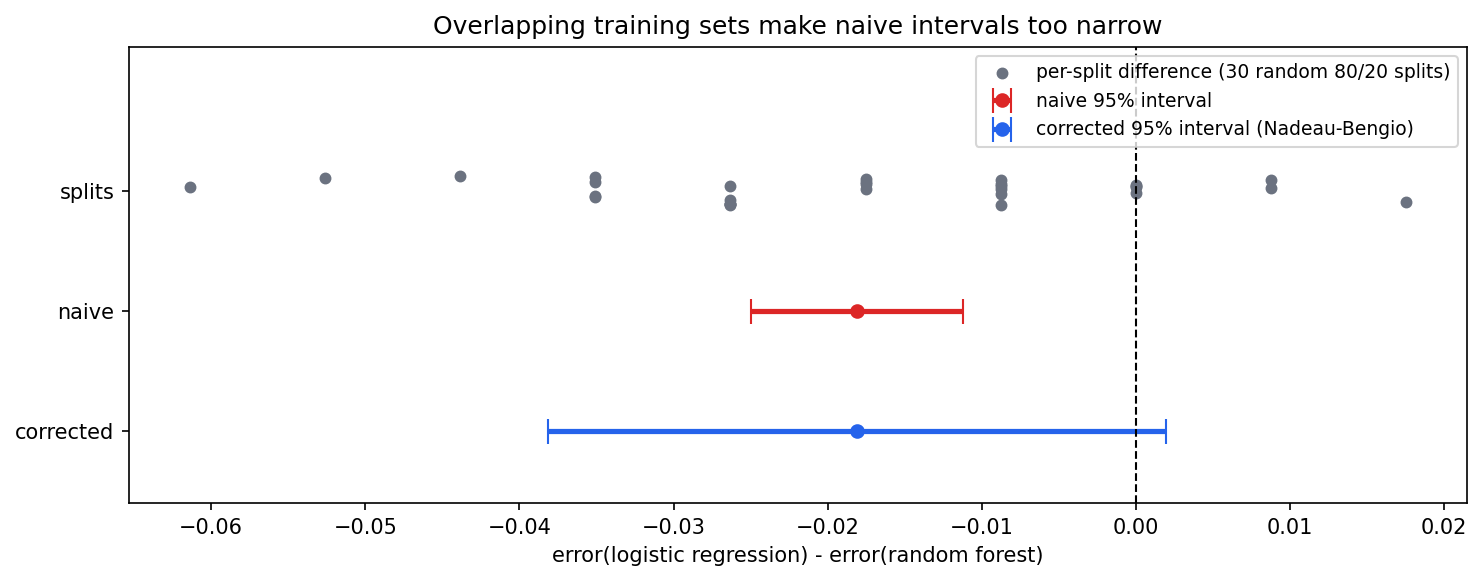
A tempting alternative is to repeat random train/test splits times, record the error differences , and run a paired -test on them. Dietterich showed this resampled -test has a badly inflated Type I error [14]: the training sets overlap heavily, so the are positively correlated and the usual standard error is far too small. Two fixes are common.
- 5×2cv paired -test [14]. Do five replications of 2-fold CV. In replication , let be the error differences on the two folds, their mean and . The statistic is compared with a distribution with 5 degrees of freedom.
- Corrected resampled -test (Nadeau and Bengio [15]). Keep random splits with test and training points, but inflate the variance to account for overlap:
where and are the mean and sample variance of the , compared with a distribution with degrees of freedom. The extra term does not shrink as grows, which is the point: more resamples of the same data cannot create more information.
Code · Python · 38 lines
import numpy as np
from scipy import stats
from sklearn.datasets import load_breast_cancer
from sklearn.model_selection import train_test_split, ShuffleSplit
from sklearn.pipeline import make_pipeline
from sklearn.preprocessing import StandardScaler
from sklearn.linear_model import LogisticRegression
from sklearn.ensemble import RandomForestClassifier

X, y = load_breast_cancer(return_X_y=True)
A = make_pipeline(StandardScaler(), LogisticRegression(max_iter=2000))
B = RandomForestClassifier(n_estimators=200, random_state=0)

# 1) McNemar's test on one held-out test set (paired predictions).
Xtr, Xte, ytr, yte = train_test_split(X, y, test_size=0.4, stratify=y,
                                      random_state=0)
ca = A.fit(Xtr, ytr).predict(Xte) == yte
cb = B.fit(Xtr, ytr).predict(Xte) == yte
n01 = int(np.sum(ca & ~cb))      # A right, B wrong
n10 = int(np.sum(~ca & cb))      # A wrong, B right
p_exact = stats.binomtest(n01, n01 + n10, 0.5).pvalue if n01 + n10 else 1.0
chi2 = (abs(n01 - n10) - 1) ** 2 / (n01 + n10) if n01 + n10 else 0.0
print(f"McNemar: n01={n01} n10={n10} chi2_cc={chi2:.3f} "
      f"p_chi2={stats.chi2.sf(chi2, 1):.3f} p_exact={p_exact:.3f}")

# 2) Corrected resampled t-test (Nadeau & Bengio) over J random splits.
J, test_frac = 30, 0.2
d = []
for tr, te in ShuffleSplit(J, test_size=test_frac, random_state=0).split(X):
    ea = np.mean(A.fit(X[tr], y[tr]).predict(X[te]) != y[te])
    eb = np.mean(B.fit(X[tr], y[tr]).predict(X[te]) != y[te])
    d.append(ea - eb)
d = np.array(d)
naive_se = np.sqrt(d.var(ddof=1) / J)
corr_se = np.sqrt(d.var(ddof=1) * (1 / J + test_frac / (1 - test_frac)))
for name, se in [("naive", naive_se), ("corrected", corr_se)]:
    t = d.mean() / se
    print(f"{name:>9} t={t:.3f}  p={2 * stats.t.sf(abs(t), J - 1):.3f}")
Our run gives , and McNemar : no evidence of a difference on one test set of 228 cases. Over 30 random 80/20 splits, logistic regression has on average about 1.8 percentage points lower error. The naive -test reports , ; the corrected test reports , (Figure 5). Same data, opposite conclusions at the 5% level: the naive test mistakes 30 heavily overlapping resamples for 30 independent experiments.
Many classifiers on many datasets
When comparing algorithms over datasets, Demšar recommends non-parametric tests on ranks [16]: the Wilcoxon signed-rank test for two classifiers, and for more the Friedman test. Rank the algorithms on each dataset (1 = best) and let be the average rank of algorithm . Under the null hypothesis that all are equivalent,
is approximately with degrees of freedom (Demšar also gives a less conservative -distributed variant). If the null is rejected, the Nemenyi post-hoc test declares two algorithms different when their average ranks differ by more than the critical difference , where comes from the Studentized range statistic divided by ; Demšar’s critical difference diagrams display the result compactly [16]. The datasets, not the folds, are the independent units here.
Benavoli, Corani, Demšar and Zaffalon argue for going further and replacing null-hypothesis significance testing with Bayesian analysis of the differences, which reports the probability that one classifier is practically better, practically equivalent within a region of practical equivalence, or worse [17]. Whatever the test, remember that a -value says nothing about how large the difference is; report effect sizes and intervals as well.
Measure decisions and probabilities
Accuracy measures the proportion correct; balanced accuracy averages per-class recall, so it is not dominated by the majority class. Macro-F1 weights classes equally when averaging classwise F1. A confusion matrix shows which errors occur. For rare positives, examine precision and recall at an operational threshold, and the full precision–recall or ROC curve when no threshold is fixed yet.
Log loss and the Brier score assess probability predictions:
where is the probability the model gave to the true class of example , and in the Brier score (binary case) is the predicted probability of the positive class and . Both are proper scoring rules: they are optimized in expectation by reporting the true probabilities. A reliability diagram compares predicted probability with observed frequency in bins. Good ranking, good accuracy and good calibration are different properties: random forests average votes and tend to push probabilities toward the middle, boosting with many rounds can push them toward the extremes, and a model can have excellent ROC AUC with poorly calibrated scores.
Fit a calibrator (scikit-learn offers sigmoid and isotonic mappings [26]) on predictions from data excluded from the corresponding base-model fitting. If observations are grouped, the calibration folds must respect those groups too. Calibration does not automatically repair domain shift.
Cluster validity as model selection
Clustering has no labels, so “validation” means something different. Theodoridis and Koutroumbas devote Chapter 16 to cluster validity because a tidy partition need not serve the task [1]. The full set of indices (silhouette, Davies–Bouldin, Calinski–Harabasz, gap statistic, BIC for mixtures) is developed alongside the algorithms in PR 07; here we place them in the validation framework of this chapter.
Internal criteria use only features and assignments. The silhouette of point compares its mean distance to its own cluster, , with the smallest mean distance to another cluster, :
It favors separation in the selected geometry. Choosing the number of clusters by maximizing an internal index is a model-selection step, exactly like tuning a hyperparameter, and a high score is not evidence that groups represent the intended semantic categories.
External criteria compare assignments with independent reference labels. The adjusted Rand index (ARI) corrects pairwise agreement for chance and is invariant to label permutations, so it does not matter which cluster is called “1.” If labels select the algorithm or the number of clusters, those labels are no longer an untouched external assessment; the separation between selection and evaluation applies here too.
Stability compares partitions after resampling or perturbation, much like the bootstrap: cluster several subsamples and measure agreement (for example ARI) on the observations they share, accounting for label permutation. Stable groups can still reflect an irrelevant camera or acquisition artifact.
Modern view
Surveys of ensemble learning. Dong, Yu, Cao, Shi and Ma survey ensemble learning broadly [21]: they review the mainstream ensemble approaches, classify them by their characteristics, list challenges and research directions for each, and discuss combining ensembles with deep learning and reinforcement learning. Ganaie, Hu, Malik, Tanveer and Suganthan review ensemble deep learning [22], organizing methods into bagging-, boosting- and stacking-based deep ensembles, negative-correlation learning, explicit versus implicit ensembles (for example snapshot or dropout-style ensembles that share weights), homogeneous versus heterogeneous members, and decision-fusion strategies. Across all of these categories the practical question is the one posed by the variance formula above: how to obtain diverse members cheaply.
Tree ensembles on tabular data. Despite the rise of deep networks, gradient-boosted trees (XGBoost [9] and its histogram-based successors) and random forests [5] remain the default for medium-sized tabular problems, which in recognition include hand-crafted descriptors, metadata and the outputs of other models. Grinsztajn, Oyallon and Varoquaux benchmarked tree-based models and deep architectures on 45 datasets and found that tree-based models remained state of the art at around 10,000 samples, attributing the gap to neural networks’ sensitivity to uninformative features, their rotation invariance, and their difficulty learning irregular functions [23].
Ensembles for uncertainty. Lakshminarayanan, Pritzel and Blundell showed that deep ensembles, several networks trained from different random initializations with a proper scoring rule, give predictive uncertainty that matched or beat approximate Bayesian methods in their experiments and degrade more gracefully on out-of-distribution inputs [24]. This links the bagging intuition (disagreement signals variance) to the Bayesian model averaging of PR 08, and it is the baseline that newer uncertainty methods are compared against.
Bias–variance revisited. Belkin, Hsu, Ma and Mandal documented double descent [25]: as capacity grows past the point where a model can interpolate the training data, test error can fall again. It does not overturn the decomposition, but it warns that “more parameters means more variance” is not a law, and that the classical U-shaped curve describes only part of the capacity range.
What cross-validation estimates. Arlot and Celisse’s survey [18] remains the reference on CV’s theory for risk estimation and model selection. Bates, Hastie and Tibshirani showed that CV estimates the average error of models fit on other training sets of the same size, not the error of the particular model in hand, and that standard CV confidence intervals can have poor coverage; they proposed a nested-CV estimate of the variance that gives intervals with better coverage [19]. Cawley and Talbot’s warning about overfitting the selection criterion [13] has grown more relevant with automated hyperparameter search, where thousands of configurations are compared on the same folds.
Comparing algorithms. Practice has moved from naive resampled -tests toward McNemar and corrected tests for one dataset [14], [15], rank-based Friedman/Nemenyi tests with critical-difference diagrams across datasets [16], and Bayesian comparisons with a region of practical equivalence [17]. Raschka’s tutorial [20] is a practical guide to all of these.
Open problems. Honest evaluation under distribution shift (new cameras, sites or populations), where no random split mirrors deployment; leakage through large pretrained models whose pretraining data may contain the test images; reliable uncertainty from ensembles that are cheap at inference time; and statistical comparison when only a single large benchmark exists. ML 11 continues these themes for deep vision models.
Key takeaways
- For squared error, expected test error = noise + bias² + variance; flexible learners such as deep trees trade bias for variance.
- Averaging predictors with pairwise correlation leaves variance : bagging and random forests help unstable learners, and decorrelating members (random feature subsets) is the lever.
- AdaBoost is greedy forward-stagewise minimization of exponential loss; gradient boosting fits trees to the negative gradient of any differentiable loss, with shrinkage and early stopping as the main regularizers.
- Voting, boosting, Bayesian model averaging and stacking combine models differently; stacking must be trained on out-of-fold predictions.
- Validation estimates a procedure: every adaptive choice belongs inside the loop, splits must respect groups and time, and nested CV is needed to report a tuned model’s performance.
- The bootstrap’s .632+ estimator corrects .632’s optimism for overfitting learners; out-of-bag scores ignore group structure.
- Do not run a naive -test on overlapping CV folds; use McNemar, 5×2cv, the corrected resampled -test, or Friedman/Nemenyi across datasets, and report effect sizes.
- Internal cluster indices, external agreement (ARI) and stability answer different questions; choosing with them is model selection.
Exercises
- Correlation floor. Derive the averaging-variance formula by expanding the variance of a sum. With , how many predictors are needed to bring the variance within 1% of its limit? What does this say about bagging very similar models?
Hint
The sum has variance terms and ordered covariance terms . The limit is ; the excess is . Requiring gives . Beyond a few dozen highly correlated models almost nothing is gained; the only way to go lower is to reduce .
- AdaBoost by hand. Five points have weights each. The first stump misclassifies exactly one of them. Compute , and the new normalized weights. What weighted error does the same stump have under the new weights, and why is that no accident?
Hint
, . Unnormalized weights: for the misclassified point and for the others; total , so the new weights are and (four times). The stump’s new weighted error is exactly : with the optimal , AdaBoost always reweights so that the last learner is no better than chance, forcing the next learner to find something new.
- Leaky folds. In the nested-CV code, replace every
GroupKFoldbyKFold(3, shuffle=True, random_state=0)(and drop thegroupsarguments). Compare the outer scores with the group-disjoint test score, and explain which deployment question each split answers.
Hint
With row-level folds, two of a subject’s three near-identical measurements are often in training when the third is validated, so the forest can recognize the subject rather than the class; inner and outer scores should rise above the independent group test. Row-level folds answer “new measurements of known subjects”; group folds answer “new subjects.”
- Bootstrap vs. CV for a stable learner. Rerun the bootstrap code with
KNeighborsClassifier(n_neighbors=15). How do resubstitution, out-of-bootstrap, .632, .632+ and 10-fold CV compare now, and why does the gap between .632 and .632+ shrink?
Hint
A 15-NN classifier no longer has zero training error, so the relative overfitting rate is much smaller, is close to 0.632, and the two estimators nearly coincide. All estimates should land within a few points of each other.
- Choosing a test. You have (a) one fixed benchmark split and the predictions of two detectors; (b) one small dataset and enough compute to retrain each model ten times; (c) five algorithms evaluated on twelve public datasets. Which test fits each case, and what are the independent units in each?
Hint
(a) McNemar’s test (or an exact binomial test) on the paired disagreements; the units are test images, and training-set variability is not captured. (b) The 5×2cv -test or the corrected resampled -test; the units are resamples, corrected for overlap. (c) Friedman test with Nemenyi post-hoc (or a Bayesian hierarchical comparison); the units are datasets.
- Clusters that mean the wrong thing. Construct (on paper or with
make_blobs) a dataset of object images that clusters strongly by camera while the class labels describe object identity. Which validity measures would expose the mismatch, and which would not?
Hint
Internal indices such as silhouette would score the camera clusters highly, because they are well separated. External ARI against object labels would be low, while ARI against camera metadata would be high. Stability would also be high, so stability alone cannot reveal that the grouping is semantically wrong.
References
-
S. Theodoridis and K. Koutroumbas, Pattern Recognition, 4th ed., Academic Press, 2009. Chapter 4 (decision trees, combining classifiers, boosting), Chapter 10 (“Supervised Learning: The Epilogue”) and Chapter 16 (“Cluster Validity”). doi
-
C. M. Bishop, Pattern Recognition and Machine Learning, Springer, 2006. Sections 1.3 and 3.2 (model selection, bias–variance) and 14.1–14.5 (Bayesian model averaging, committees, boosting, trees, conditional mixtures). official book and PDF
-
S. Geman, E. Bienenstock and R. Doursat, “Neural networks and the bias/variance dilemma,” Neural Computation, vol. 4, no. 1, pp. 1–58, 1992. doi
-
L. Breiman, “Bagging predictors,” Machine Learning, vol. 24, no. 2, pp. 123–140, 1996. doi
-
L. Breiman, “Random forests,” Machine Learning, vol. 45, no. 1, pp. 5–32, 2001. doi
-
Y. Freund and R. E. Schapire, “A decision-theoretic generalization of on-line learning and an application to boosting,” Journal of Computer and System Sciences, vol. 55, no. 1, pp. 119–139, 1997. doi
-
J. Friedman, T. Hastie and R. Tibshirani, “Additive logistic regression: A statistical view of boosting (with discussion),” The Annals of Statistics, vol. 28, no. 2, 2000. doi
-
J. H. Friedman, “Greedy function approximation: A gradient boosting machine,” The Annals of Statistics, vol. 29, no. 5, 2001. doi
-
T. Chen and C. Guestrin, “XGBoost: A scalable tree boosting system,” in Proc. 22nd ACM SIGKDD International Conference on Knowledge Discovery and Data Mining, pp. 785–794, 2016. doi
-
D. H. Wolpert, “Stacked generalization,” Neural Networks, vol. 5, no. 2, pp. 241–259, 1992. doi
-
B. Efron and R. Tibshirani, “Improvements on cross-validation: The .632+ bootstrap method,” Journal of the American Statistical Association, vol. 92, no. 438, pp. 548–560, 1997. doi
-
S. Varma and R. Simon, “Bias in error estimation when using cross-validation for model selection,” BMC Bioinformatics, vol. 7, 91, 2006. doi
-
G. C. Cawley and N. L. C. Talbot, “On over-fitting in model selection and subsequent selection bias in performance evaluation,” Journal of Machine Learning Research, vol. 11, pp. 2079–2107, 2010. JMLR
-
T. G. Dietterich, “Approximate statistical tests for comparing supervised classification learning algorithms,” Neural Computation, vol. 10, no. 7, pp. 1895–1923, 1998. doi
-
C. Nadeau and Y. Bengio, “Inference for the generalization error,” Machine Learning, vol. 52, no. 3, pp. 239–281, 2003. doi
-
J. Demšar, “Statistical comparisons of classifiers over multiple data sets,” Journal of Machine Learning Research, vol. 7, pp. 1–30, 2006. JMLR
-
A. Benavoli, G. Corani, J. Demšar and M. Zaffalon, “Time for a change: A tutorial for comparing multiple classifiers through Bayesian analysis,” Journal of Machine Learning Research, vol. 18, no. 77, pp. 1–36, 2017. JMLR
-
S. Arlot and A. Celisse, “A survey of cross-validation procedures for model selection,” Statistics Surveys, vol. 4, pp. 40–79, 2010. doi
-
S. Bates, T. Hastie and R. Tibshirani, “Cross-validation: What does it estimate and how well does it do it?,” Journal of the American Statistical Association, vol. 119, no. 546, pp. 1434–1445, 2024. doi
-
S. Raschka, “Model evaluation, model selection, and algorithm selection in machine learning,” arXiv:1811.12808, 2018. arXiv
-
X. Dong, Z. Yu, W. Cao, Y. Shi and Q. Ma, “A survey on ensemble learning,” Frontiers of Computer Science, vol. 14, no. 2, pp. 241–258, 2020. doi
-
M. A. Ganaie, M. Hu, A. K. Malik, M. Tanveer and P. N. Suganthan, “Ensemble deep learning: A review,” Engineering Applications of Artificial Intelligence, vol. 115, 105151, 2022. doi
-
L. Grinsztajn, E. Oyallon and G. Varoquaux, “Why do tree-based models still outperform deep learning on typical tabular data?,” in Advances in Neural Information Processing Systems (NeurIPS) Datasets and Benchmarks Track, 2022 (arXiv:2207.08815). arXiv
-
B. Lakshminarayanan, A. Pritzel and C. Blundell, “Simple and scalable predictive uncertainty estimation using deep ensembles,” in Advances in Neural Information Processing Systems (NIPS), 2017 (arXiv:1612.01474). arXiv
-
M. Belkin, D. Hsu, S. Ma and S. Mandal, “Reconciling modern machine-learning practice and the classical bias–variance trade-off,” Proceedings of the National Academy of Sciences, vol. 116, no. 32, pp. 15849–15854, 2019. doi
-
scikit-learn developers, scikit-learn User Guide: ensemble methods, cross-validation, probability calibration and clustering performance evaluation.
-
NumPy developers, “numpy.linalg.lstsq,” API documentation, accessed 2026-11-05. documentation
Check your understanding
This tutorial has 6 exercises. Can you solve them without opening the hints?
Go to the exercises ↑Next PR 10 · Recognition Capstone: Rejection, Shift and Learned Features · 32 min