PR 01 · Patterns, Probability and Bayes Decisions
Needs: ML 01B · Probability and Information Theory
Navigate: this page and this track: Navigate: this page and this track
On this page
- What you’ll learn1 min
- The big picture2 min
- Start with the experiment1 min
- Bayes’ rule connects evidence and belief3 min
- Minimum-error decisions1 min
- Loss matrices and minimum risk2 min
- The reject option2 min
- Discriminant functions and decision regions1 min
- The Gaussian case: LDA and QDA boundaries3 min
- ROC analysis and the Neyman–Pearson view3 min
- Where the assumptions can fail1 min
- Modern view3 min
- Key takeaways1 min
- Exercises2 min
- References
Pattern Recognition
Explore this chapter 1 interactive experiment
Move a decision boundary by changing class frequency and the cost of a false alarm.
What you’ll learn
- Turn a recognition problem into observations, features, predictions and actions, and decide what one “sample” means.
- Distinguish a class prior, a class likelihood and a class posterior, and see how a change in the prior moves a decision boundary.
- Derive the minimum-error rule, the minimum-risk rule for any loss matrix, and Chow’s reject rule.
- Write classifiers as discriminant functions and derive the linear (LDA) and quadratic (QDA) boundaries of the Gaussian case.
- Read ROC and precision–recall curves, connect them to the Neyman–Pearson criterion, and choose an operating point from costs.
The big picture
A camera records a manufactured component. A system measures its shape, estimates whether it is defective, and decides whether to send it for manual inspection. These are different stages. The recorded pixels are observations; shape measurements are features; a defect probability is a prediction; sending the part to inspection is an action. Bayes decision theory is the part of pattern recognition that connects the last two: given what we believe, what should we do?
This track follows the classic pattern-recognition textbooks: Duda, Hart and Stork’s Pattern Classification [1], Bishop’s Pattern Recognition and Machine Learning [2], and Theodoridis and Koutroumbas’s Pattern Recognition [3], with Hastie, Tibshirani and Friedman [4] for the statistical view. The chapters use original examples and derivations; the textbooks are where to go for longer proofs. Bayes decision theory comes first in all of them because every later method can be judged against it: a classifier is good to the extent that it approximates the decision the Bayes rule would take if we knew the true distributions.
Recognition is not limited to images. An observation can be a sound recording, a sequence of pen strokes or a document. Classification predicts categories, regression predicts quantities, and clustering discovers groups without labels. This chapter is about classification, but the way of thinking (model the uncertainty, then choose the action with the lowest expected cost) carries over to all three.
Start with the experiment
Plain version. Before any formula, write down what one sample is and how the data were collected. Most surprising failures of recognition systems come from this step, not from the classifier.
One image, one patient, one video and one crop of a video are different sampling units. If twenty frames come from the same recording, treating them as twenty independent cases can make a test look much easier than deployment, because the test frames are near-copies of training frames.
Precise version. A recognition pipeline can be written as
Here is a raw observation (an image, a waveform); is the preprocessing and feature extraction that maps it to a feature vector ; is one of classes; is the model’s belief about the class; and is the action finally taken. Learning adjusts the parameters of and of the probability model from training samples; validation samples choose settings such as thresholds and regularization; a held-out test set estimates the performance of the whole chosen procedure once (PR 09 treats this carefully: validation and ensembles).
Handcrafted features (edge histograms, shape moments) and learned embeddings (the output of a pretrained network) occupy the same slot . Changing the feature extractor changes which information the classifier receives. Information removed by cropping, quantization or pooling cannot be recovered by any classifier downstream, however clever. In decision-theoretic language: the Bayes error of the problem is defined relative to the features, and a poor raises the floor that no classifier can go below.
Bayes’ rule connects evidence and belief
Plain version. Bayes’ rule says how to update “how common is each class” into “how likely is each class for this object”, using “how typical is this measurement for each class”.
Precise version. Let the classes be . Bayes’ rule gives
- The prior is the probability of class before examining this observation, for example the fraction of defective parts on the production line.
- The likelihood (or class-conditional density) describes how measurements are distributed within class .
- The evidence is the overall density of ; it is the same for every class and only normalizes.
- The posterior is the probability of class after observing .
For continuous measurements, a likelihood is a density. Its value need not lie between zero and one, and it is not the probability of observing that exact real number. Posterior class probabilities do lie in and sum to one over . Confusing the two directions of conditioning, versus , is the classic base-rate error that the code example below makes concrete.
Because the evidence is shared, a decision only needs the products . Figure 1 shows what that means geometrically for two one-dimensional Gaussian classes: the boundary sits where the two prior-weighted likelihoods cross. When the prior of class drops from to , its weighted curve shrinks, and the boundary moves towards ‘s mean: the system now needs stronger evidence before declaring the rarer class.
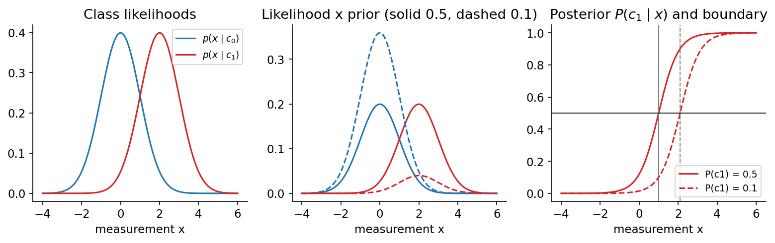
For the unit-variance case in Figure 1 the boundary has a closed form. With means , and variance , the log ratio of the weighted likelihoods is , which is zero at . That is for equal priors and for .
Code: rare events change the posterior
This NumPy example uses hypothetical inspection statistics: a detector flags of defective parts (sensitivity) and of good parts (false-positive rate), and of parts are defective. It computes the posterior after a positive and after a negative detector output, then compares the minimum-error and minimum-risk actions (derived in the next sections).
Code · Python · 18 lines
import numpy as np

prior = 0.02
sensitivity = 0.90
false_positive_rate = 0.08
p_positive = (sensitivity * prior /
              (sensitivity * prior + false_positive_rate * (1 - prior)))
p_negative = ((1 - sensitivity) * prior /
              ((1 - sensitivity) * prior + (1 - false_positive_rate) * (1 - prior)))
p = np.array([p_negative, p_positive])
c_fp, c_fn = 1.0, 9.0
threshold = c_fp / (c_fp + c_fn)
risks = np.column_stack([c_fn * p, c_fp * (1 - p)])
decisions = risks.argmin(axis=1)
assert np.array_equal(decisions, (p > threshold).astype(int))
print("posteriors [negative observation, positive observation]:", p)
print("minimum-risk actions:", decisions, "threshold:", threshold)
print("minimum-error actions:", (p > 0.5).astype(int))
The output is a posterior of about after a negative flag and only after a positive one. A positive observation does not imply a defect probability: sensitivity conditions on the true class, while the posterior conditions on the observation, and with a prior most positive flags come from the large pool of good parts. Under equal costs, neither observation leads to “defective” (). With a missed defect costing nine times as much as an unnecessary inspection, the threshold drops to and a positive flag does lead to inspection. The probability model did not change; only the decision rule did.
Minimum-error decisions
Plain version. If every mistake costs the same, always pick the class that is most probable for this observation. No other rule makes fewer mistakes on average.
Precise version. A decision rule assigns each to a class, which partitions feature space into decision regions , where . The probability of error is
Here is the posterior of the class we chose. The integrand is non-negative and does not depend on the rule, so the integral is minimized by minimizing separately at every , that is, by choosing
This is the maximum a posteriori (MAP) rule or Bayes classifier. Its error,
is the Bayes error: the lowest error any classifier can achieve with these features. It is zero only when the classes do not overlap in feature space. A classifier with test error on a problem whose Bayes error is is close to optimal; the same on a problem with Bayes error leaves a lot on the table. We rarely know the Bayes error of a real task, but thinking about it separates two different questions: “are my features informative enough?” (the Bayes error) and “does my classifier extract what the features contain?” (the gap above it).
For two classes the MAP rule becomes a likelihood-ratio test:
Choose when the ratio exceeds the threshold on the right, otherwise. The data enter only through ; priors and, as we will see next, costs only move the threshold. This is why one score can serve many decision policies.
Loss matrices and minimum risk
Plain version. Some mistakes are worse than others. Assign a cost to each kind of mistake, compute the average cost of each possible action given the current beliefs, and take the cheapest action.
Precise version. Let the available actions be (usually “decide class ”, possibly also “reject”). A loss matrix gives the cost of taking action when the true class is . The conditional risk of an action is its expected loss under the posterior:
The overall risk is minimized by the same pointwise argument as before, so this Bayes decision rule achieves the minimum possible expected loss, the Bayes risk [1, 2]. With the zero-one loss ( if , otherwise), and the rule reduces to MAP.
For two classes, write for the cost of deciding when the truth is (a false positive) and for deciding when the truth is (a false negative). Choosing is cheaper when , which rearranges to
This ratio form assumes positive class priors and , as in ordinary classification costs. If that difference is zero, compare the risks directly; if negative, dividing reverses the inequality. With free correct decisions, doubling the false-negative cost has the same effect as doubling the prior odds , not the positive-class probability alone. The two priors must still sum to one. With correct decisions free (), , and , the rule becomes a threshold on the posterior:
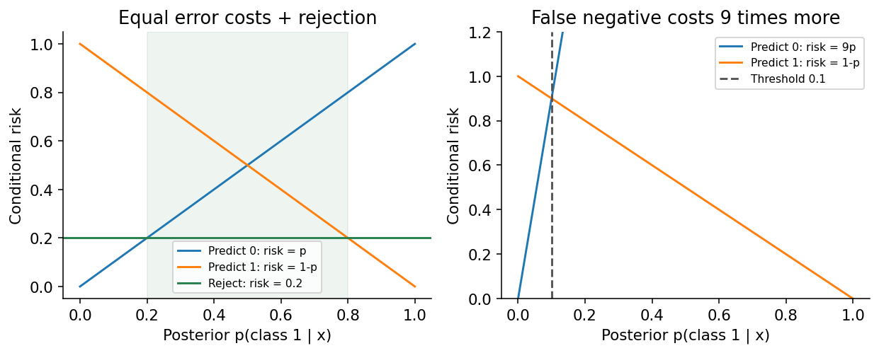
When missing a defect costs nine times as much as an unnecessary inspection, the threshold is , not (Figure 2, right).
Two remarks matter in practice. First, a loss matrix is a modelling decision, often made by people outside the machine-learning team (clinicians, safety engineers, product owners); write it down explicitly so that it can be reviewed. Second, the posterior threshold is only meaningful if the posterior is calibrated, meaning that among cases given probability , about really are positive. Many modern classifiers are not, which is one theme of the Modern view below.
The reject option
Plain version. When the system is unsure, it can hand the case to a person. Refusing to decide has a fixed cost; deciding has an expected cost that is high when the posterior is spread out. Refuse exactly when deciding is expected to cost more.
Precise version. Add an action with constant loss regardless of the true class, and keep the zero-one loss for the classification actions. The best classification action has risk , so the Bayes rule becomes Chow’s rule [5]:
If rejection costs , the system accepts only when the top posterior is at least (Figure 2, left). Two edge cases help intuition. If (asking a person is free), the system rejects everything that is not certain. If , it never rejects, because the top posterior is always at least .
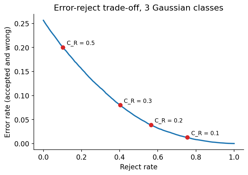
Chow showed that sweeping the threshold traces an error–reject trade-off curve: each extra percent of rejected samples buys a reduction in the error on the remaining ones, with diminishing returns [5]. Figure 3 shows it for three overlapping Gaussian classes whose true posteriors are known. Without rejection about a quarter of all samples are misclassified; rejecting the least certain cuts the error on all samples to about .
Code: Chow’s rule
Code · Python · 20 lines
import numpy as np

rng = np.random.default_rng(2)
means = np.array([[0, 0], [2, 0], [1, 1.7]])
y = rng.integers(0, 3, 20000)
X = means[y] + rng.normal(0, 1, (len(y), 2))

# exact posteriors: equal priors, identity covariance
logits = -0.5 * ((X[:, None, :] - means[None]) ** 2).sum(-1)
post = np.exp(logits - logits.max(1, keepdims=True))
post /= post.sum(1, keepdims=True)
pred, pmax = post.argmax(1), post.max(1)

for c_r in [0.5, 0.3, 0.2, 0.1]:
    accept = pmax >= 1 - c_r                     # Chow's rule
    reject_rate = 1 - accept.mean()
    err_accepted = np.mean(pred[accept] != y[accept])
    risk = np.mean(np.where(accept, pred != y, c_r))
    print(f"C_R={c_r}: reject {reject_rate:.3f}, "
          f"error on accepted {err_accepted:.3f}, average loss {risk:.3f}")
With this seed, rejects about of samples and leaves an error of about among the accepted ones; rejects about and leaves about . The average loss always falls as falls because the reject action itself becomes cheaper. Subtracting the max logit before exponentiating (logits.max) is the standard trick that keeps the softmax numerically stable.
Rejection helps only when the uncertainty estimate is meaningful. Chow’s rule handles ambiguity: observations that lie between known classes. It does not handle novelty: an object of a kind never seen in training can land far from every class and still receive a confident posterior, because posteriors are normalized over the known classes only. Detecting such inputs is the subject of open-set recognition and out-of-distribution detection (Modern view).
Discriminant functions and decision regions
Plain version. A classifier can be written as a set of scoring functions, one per class: compute every score and pick the largest. Many different scores give the same decisions.
Precise version. A classifier is defined by discriminant functions and the rule “assign to if for all ” [1]. The Bayes minimum-error classifier is obtained with , but any monotonically increasing function applied to all discriminants leaves every decision unchanged. Three equivalent choices are therefore
The log form is the one used in practice: it turns products of many small densities into sums and avoids numerical underflow. For minimum risk, use .
The decision boundary between and is the set where and both are larger than all other scores. For two classes a single function suffices, a dichotomizer:
This is the log-likelihood ratio plus the log prior odds. It also equals the logit of the posterior, because with the logistic sigmoid . Remember this identity: in PR 03, logistic regression models directly as a linear function instead of deriving it from densities.
The view through discriminants is useful because it separates what the classifier computes (the shape of the boundaries) from how it was obtained (densities, direct fitting, margins). Linear discriminants produce boundaries that are hyperplanes and regions that are convex; quadratic discriminants produce conics in 2-D and hyperquadrics in general. The Gaussian case shows exactly when each arises.
The Gaussian case: LDA and QDA boundaries
Plain version. If each class looks like a “cloud” shaped like a multivariate Gaussian, the Bayes rule measures how far is from each cloud’s center, in units that respect the cloud’s shape. When all clouds have the same shape, the boundaries are straight; when shapes differ, they bend.
Precise version. Suppose with mean and covariance matrix (symmetric, positive definite):
where is the determinant. The log discriminant is
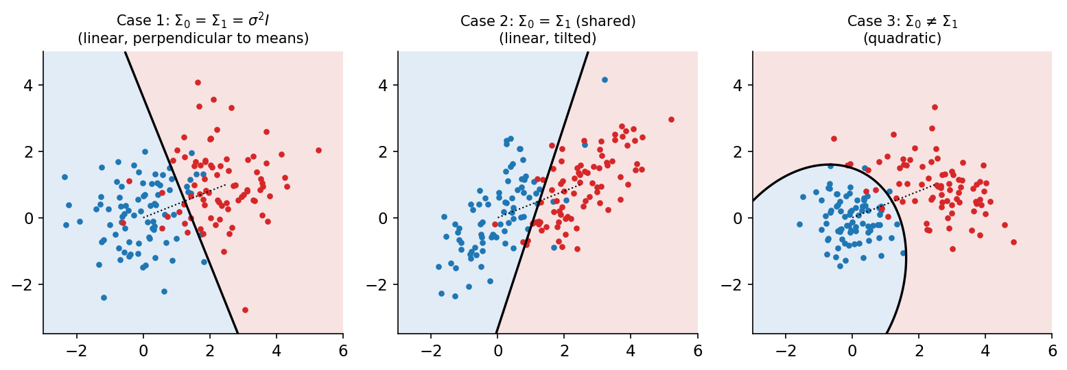
after dropping the constant shared by all classes. The quadratic form is the squared Mahalanobis distance from to : Euclidean distance after “whitening” the class so its cloud becomes a unit sphere. Three cases, shown in Figure 4, cover what happens [1, 4].
Case 1: for all . Features are uncorrelated with equal variance . Expanding and dropping the class-independent gives a linear discriminant
The boundary between classes and is the hyperplane with and
It is perpendicular to the line joining the means. With equal priors it passes through their midpoint, and the classifier is exactly the minimum-distance (nearest-mean) classifier of IP 13. Unequal priors slide the plane away from the more probable mean.
Case 2: shared by all classes. The quadratic term is again common and cancels, leaving
The boundaries are still hyperplanes, with , but no longer perpendicular to the mean difference: they tilt to follow the shared correlation (Figure 4, middle). This is linear discriminant analysis (LDA) in its probabilistic form. With equal priors it is a minimum-Mahalanobis-distance classifier. The direction is the same as the one Fisher derived from a projection criterion in 1936, which PR 03 re-derives.
Case 3: arbitrary . Nothing cancels:
The boundaries are hyperquadrics: lines, parabolas, ellipses or hyperbolas in 2-D. This is quadratic discriminant analysis (QDA). In Figure 4 (right) the tight blue class is enclosed by an ellipse, because a point far from the blue mean in any direction is better explained by the broad red class. A region can even be disconnected, which never happens for linear discriminants.
For two classes with a shared covariance and equal priors, the Bayes error has a closed form,
where is the standard normal cumulative distribution function and is the Mahalanobis distance between the means. Two classes three standard deviations apart () still give unavoidable error. This formula is a good sanity check for any classifier you train on Gaussian toy data.
Which case should you use? It is a bias–variance choice. A full covariance per class has free entries per class; with that is numbers per class, which needs far more samples than many datasets have. Sharing one covariance (LDA), restricting to diagonals (which gives Gaussian naive Bayes) or shrinking towards a simple target trades flexibility for stability. Estimating these parameters is the subject of the next chapter, PR 02: density estimation.
Code: Gaussian discriminants from scratch
This example fits Gaussian class models, evaluates the log discriminants with a Cholesky factorization (never an explicit inverse), and checks that the decisions match scikit-learn’s LinearDiscriminantAnalysis and QuadraticDiscriminantAnalysis on the Case 3 data of Figure 4.
Code · Python · 37 lines
import numpy as np
from sklearn.discriminant_analysis import (LinearDiscriminantAnalysis,
                                           QuadraticDiscriminantAnalysis)

rng = np.random.default_rng(0)
means = [np.array([0.0, 0.0]), np.array([2.5, 1.0])]
covs = [np.array([[0.4, 0.0], [0.0, 0.4]]), np.array([[2.0, -0.6], [-0.6, 1.0]])]
X = np.vstack([rng.multivariate_normal(m, S, 300) for m, S in zip(means, covs)])
y = np.repeat([0, 1], 300)

def fit_gaussians(X, y, shared):
    params = []
    pooled = sum(np.cov(X[y == k].T, bias=True) * (y == k).sum()
                 for k in (0, 1)) / len(y)
    for k in (0, 1):
        Xk = X[y == k]
        S = pooled if shared else np.cov(Xk.T, bias=True)
        params.append((Xk.mean(0), S, len(Xk) / len(y)))
    return params

def discriminants(X, params):
    g = []
    for mu, S, prior in params:
        L = np.linalg.cholesky(S)               # S = L L^T
        z = np.linalg.solve(L, (X - mu).T)      # whitened residuals
        maha = (z ** 2).sum(0)                  # squared Mahalanobis distance
        logdet = 2 * np.log(np.diag(L)).sum()
        g.append(-0.5 * maha - 0.5 * logdet + np.log(prior))
    return np.stack(g, axis=1)

for shared, ref in [(True, LinearDiscriminantAnalysis(store_covariance=True)),
                    (False, QuadraticDiscriminantAnalysis())]:
    mine = discriminants(X, fit_gaussians(X, y, shared)).argmax(1)
    theirs = ref.fit(X, y).predict(X)
    name = "LDA (shared)" if shared else "QDA (separate)"
    print(f"{name}: training error {np.mean(mine != y):.3f}, "
          f"agrees with scikit-learn on {np.mean(mine == theirs):.1%} of points")
Both hand-written classifiers agree with scikit-learn on every point. On these data, whose true covariances differ, QDA’s training error () is below LDA’s (). That is training error, though: with few samples in high dimensions the ordering often reverses on held-out data.
ROC analysis and the Neyman–Pearson view
Plain version. A two-class score can be cut at many thresholds. Each threshold trades catching more positives against raising more false alarms. The ROC curve draws all those trade-offs at once, so you can pick the threshold later, when costs or priors are known.
Precise version. Let be any score where larger values favor (the log-likelihood ratio, a posterior, a network logit), and decide when . For each threshold define
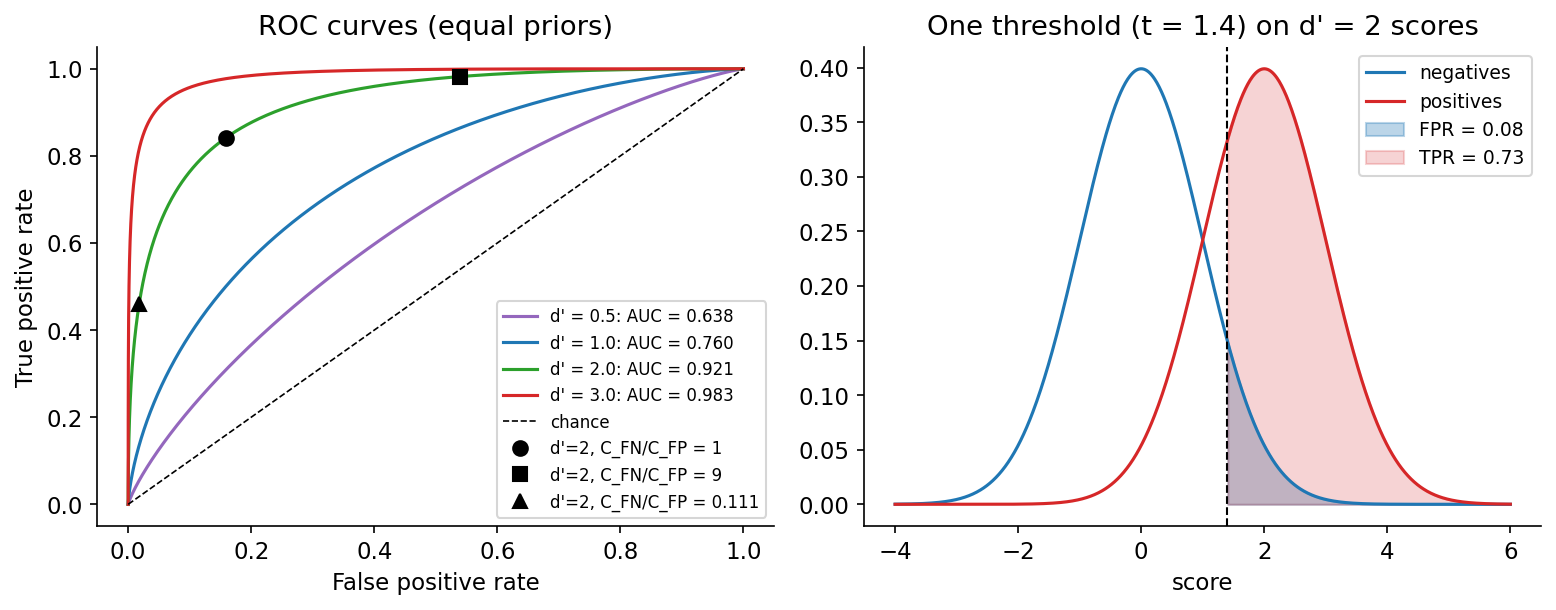
The true-positive rate (sensitivity, recall) is the fraction of positives caught; the false-positive rate ( specificity) is the fraction of negatives flagged. The receiver operating characteristic (ROC) curve plots TPR against FPR as sweeps from to [7]. A useless score lies on the diagonal; a perfect one passes through the top-left corner. Because both rates condition on the true class, the ROC curve does not change when the class priors change.
The Neyman–Pearson criterion. Sometimes costs are hard to state but a constraint is easy: “at most false alarms”. The Neyman–Pearson lemma [6] says that among all decision rules with , the one with the highest TPR is a likelihood-ratio test , with chosen so the false-positive rate equals (with randomization at the boundary if needed). So the ROC curve of the likelihood ratio is the best achievable curve; any other score’s ROC lies on or below it. Both the Bayes rule and the Neyman–Pearson rule are likelihood-ratio tests; they differ only in how the threshold is chosen.
Choosing an operating point from costs. The expected cost per sample at threshold is
Points of equal cost lie on straight iso-cost lines in ROC space with slope ; all these lines have the same fixed slope. Slide the line toward higher TPR (a larger vertical intercept) until it last touches an achievable point; that point minimizes cost [7]. For the likelihood-ratio score this tangent point is exactly the Bayes threshold derived earlier.
Area under the curve. The AUC summarizes the curve in one number. It equals the probability that a randomly chosen positive receives a higher score than a randomly chosen negative (ties counted half) [7]. For two unit-variance Gaussian score distributions separated by standard deviations, : Figure 5 shows gives . AUC ignores costs, priors and calibration, so two classifiers with the same AUC can have very different costs at the threshold you actually deploy.
Precision–recall curves. When positives are rare (fraud, defects, small objects in detection), a small FPR can still mean many false alarms in absolute numbers, because negatives are so numerous. Precision depends on the prior and exposes this. Davis and Goadrich [8] proved that one curve dominates another in ROC space if and only if it dominates in precision–recall space, and that linear interpolation between PR points is not valid. Saito and Rehmsmeier [9] showed with simulations and published studies that for imbalanced data the PR plot is more informative than ROC. Object-detection benchmarks report average precision for this reason (see DLCV 03).
Code: ROC, AUC and the cost-optimal threshold
Code · Python · 25 lines
import numpy as np
from sklearn.metrics import roc_auc_score, roc_curve

rng = np.random.default_rng(1)
n_neg, n_pos = 9000, 1000                       # prevalence 10%
scores = np.r_[rng.normal(0, 1, n_neg), rng.normal(2, 1, n_pos)]
labels = np.r_[np.zeros(n_neg), np.ones(n_pos)]

fpr, tpr, thr = roc_curve(labels, scores)
auc = roc_auc_score(labels, scores)
# Mann-Whitney view of AUC: P(score_pos > score_neg)
pos, neg = scores[labels == 1], scores[labels == 0]
auc_pairs = (pos[:, None] > neg[None, :]).mean()
print(f"AUC = {auc:.4f}, pairwise estimate = {auc_pairs:.4f}")

# choose the operating point with minimum expected cost per sample
c_fp, c_fn, prior = 1.0, 9.0, n_pos / (n_pos + n_neg)
cost = c_fp * fpr * (1 - prior) + c_fn * (1 - tpr) * prior
i = np.argmin(cost)
print(f"best threshold {thr[i]:.2f}: FPR {fpr[i]:.3f}, TPR {tpr[i]:.3f}, "
      f"expected cost {cost[i]:.3f}")
# Bayes threshold from the true model: predict 1 when the likelihood ratio
# exceeds c_fp (1 - prior) / (c_fn prior); for unit Gaussians, log LR = 2s - 2
t_bayes = (np.log(c_fp * (1 - prior) / (c_fn * prior)) + 2) / 2
print(f"Bayes threshold from the true densities: {t_bayes:.2f}")
The empirical AUC () matches the pairwise-ranking estimate exactly, and is close to the theoretical . With a prior and a 9:1 cost ratio, prior odds and cost ratio cancel, so the Bayes threshold is ; the empirical search finds . In a real project the threshold search must run on validation data, never on the test set.
Where the assumptions can fail
The Bayes rule is optimal relative to the assumed distributions and the specified loss. Each ingredient can be wrong in deployment.
Prior shift. Class frequencies may differ between the training set and deployment, for example between two factories or between a balanced research dataset and a real clinic. If the class-conditional distributions stay fixed (label shift), the posterior can be corrected without retraining: multiply each posterior by the ratio of new to old priors and renormalize,
When the new priors are unknown, Saerens, Latinne and Decaestecker [10] estimate them with an EM procedure on the unlabeled deployment data, and Lipton, Wang and Smola’s black-box shift estimation [11] estimates them from a classifier’s confusion matrix. If a new camera changes the likelihoods themselves (covariate or concept shift), a prior correction is not enough.
Miscalibrated posteriors. Every threshold in this chapter assumes that means what it says. Scores from SVMs, boosted trees or deep networks are often systematically over- or under-confident; recalibration on held-out data (Platt scaling, isotonic regression, temperature scaling) is a standard fix [12, 14].
Label noise and proxies. A label may record an imperfect inspection rather than physical truth. The model then learns the inspector’s posterior, not the world’s.
Single-number summaries. Two classifiers with identical accuracy can have different false-negative rates and very different expected loss. Report the confusion matrix, the operating point and the costs.
Modern view
Bayes decision theory is more than fifty years old, and its vocabulary (posterior, risk, reject, operating point) is now the vocabulary of trustworthy deep learning. Research since 2017 has mostly been about making the inputs to the Bayes rule trustworthy when the classifier is a large network.
Calibration. Guo et al. [12] found that modern deep networks were much more overconfident than the shallower networks of a decade earlier. They related this to depth, width, weight decay and batch normalization, and showed that temperature scaling (dividing all logits by one scalar fitted on validation data, a one-parameter version of Platt scaling) is surprisingly effective. Minderer et al. [13] revisited the question for 2021-era image classifiers and found that the most recent models, notably those not using convolutions, are among the best calibrated, and that the earlier trend of calibration decaying with model size or under distribution shift is less pronounced. The survey by Silva Filho et al. [14] is the best entry point: it covers proper scoring rules and calibration metrics, reliability diagrams, and a comprehensive account of post-hoc calibration methods for binary and multiclass problems. Gawlikowski et al. [23] review the wider field of uncertainty in neural networks, separating reducible model uncertainty from irreducible data uncertainty and covering Bayesian networks, ensembles and test-time augmentation.
Rejection and selective classification. Chow’s reject rule [5] has been rediscovered as selective classification. Geifman and El-Yaniv [16] showed how to wrap a trained network with a rejection threshold chosen so that the risk on accepted samples stays below a user-specified level with high probability, trading coverage for guaranteed accuracy. The survey by Hendrickx et al. [15] formalizes two kinds of rejection, ambiguity rejection (Chow’s case) and novelty rejection (inputs unlike the training data), reviews how to evaluate a model’s predictive and rejective quality together, and categorizes the architectures used to learn models with a reject option.
Distribution-free guarantees. Conformal prediction replaces a single label with a set of labels that is guaranteed to contain the true class with a chosen probability, such as , under the sole assumption that calibration and test data are exchangeable. Angelopoulos and Bates [17] give a hands-on introduction with code. Large prediction sets play the role of rejection: the model is telling you that it cannot narrow things down.
Open-set recognition and out-of-distribution detection. A posterior normalized over known classes cannot say “none of the above”. Geng, Huang and Chen [18] survey open-set recognition: definitions, model families, datasets and evaluation, and its relationship to classification with reject option and to zero- and few-shot learning. Yang et al. [19] unify anomaly detection, novelty detection, open-set recognition, out-of-distribution detection and outlier detection as sub-tasks of one generalized OOD detection framework. Two results connect directly to this chapter. Hendrycks and Gimpel [20] showed that the maximum softmax probability, Chow’s statistic, is a strong baseline for detecting both misclassified and out-of-distribution inputs. Vaze et al. [21] found that a classifier’s ability to say “none of the above” is highly correlated with its closed-set accuracy, so improving the ordinary classifier improves open-set performance. Lee et al. [22] fit class-conditional Gaussians with a shared covariance (exactly Case 2 / LDA above) to the features of a pretrained network and use the Mahalanobis distance as a confidence score. A 1970s-style generative classifier, placed on top of learned features, remains a competitive OOD detector.
Open problems. Costs are rarely known precisely, and they change over time; calibration measured on one distribution may not transfer to another; and guarantees such as conformal coverage are marginal (on average over inputs) rather than conditional on a particular input or subgroup. Deciding what the loss matrix should be, and who decides, remains a human question that no estimator answers.
Key takeaways
- A recognition system maps observations to features, features to beliefs, and beliefs to actions; the sampling unit and data split are part of the problem definition.
- Prior, likelihood and posterior answer different questions. Rare classes need strong evidence: a -sensitive test at prevalence gives a posterior below .
- Maximum posterior minimizes the error rate; minimum conditional risk handles any loss matrix. For two classes both are likelihood-ratio tests whose threshold depends on priors times costs.
- Chow’s rule rejects when the top posterior falls below ; it handles ambiguity, not novelty.
- Discriminant functions are defined up to a monotone transform. Gaussian classes give linear boundaries when covariances are shared (LDA) and quadratic ones when they differ (QDA).
- ROC curves separate the score from the threshold; the Neyman–Pearson lemma makes the likelihood ratio the optimal score; PR curves are more informative when positives are rare.
- All of this relies on calibrated probabilities and stable priors, which modern work on calibration, selective classification, conformal prediction and OOD detection tries to secure.
Exercises
- Asymmetric costs. Derive the binary decision threshold on the posterior when a false positive costs four and a false negative costs one. Which class does the rule now favor, and why?
Hint
Choose when , so the threshold is . False alarms are now the expensive mistake, so the rule needs strong evidence before saying “positive”.
- Reject or not. For posterior and reject cost , choose the minimum-risk action under zero-one classification loss. For which values of would the answer change?
Hint
The best classification risk is , so reject. The system classifies (as ) when .
- A moving boundary. Two 1-D classes have and . Find the minimum-error boundary for equal priors and for . Then find the minimum-risk boundary for equal priors when a false negative costs four times a false positive.
Hint
The log-likelihood ratio is . Equal priors: . With : , so . With : , so . The prior and the cost act through the same threshold, in opposite directions here.
- Mahalanobis versus Euclidean. Two classes share with means and and equal priors. Classify with the Euclidean nearest-mean rule and with the Bayes (LDA) rule. Explain the disagreement.
Hint
Euclidean squared distances: to and to , so nearest-mean says . Mahalanobis: to and to , a tie: lies exactly on the LDA boundary. The first feature varies a lot, so a 2-unit offset along it is weak evidence; the Euclidean rule over-weights it.
- ROC from scratch. Using NumPy only, compute the ROC curve and the AUC of the scores in the ROC code example by sorting the scores, and verify against
roc_auc_score. Then change the prevalence to and explain which of ROC, AUC and precision at a fixed threshold change.
Hint
Sort scores in decreasing order; cumulative sums of labels give TP counts and of labels give FP counts; integrate TPR over FPR with the trapezoid rule. ROC and AUC depend only on the two class-conditional score distributions, so they stay (up to sampling noise) the same; precision at a fixed threshold falls sharply because false positives now come from a much larger pool of negatives.
- The sampling unit. A test set contains adjacent frames from the same videos used for training. Explain what its accuracy estimates, and propose a split that estimates performance on new videos, new cameras or new subjects.
Hint
It estimates accuracy on near-duplicates of training frames (an interpolation task). Split by recording (group-wise splitting), and, if deployment will meet new cameras or people, hold out entire cameras or subjects as well.
References
- R. O. Duda, P. E. Hart and D. G. Stork, Pattern Classification, 2nd ed., Wiley, 2001 (Ch. 2, Bayesian decision theory). publisher page
- C. M. Bishop, Pattern Recognition and Machine Learning, Springer, 2006 (Sections 1.2 and 1.5). official page and free PDF
- S. Theodoridis and K. Koutroumbas, Pattern Recognition, 4th ed., Academic Press, 2008 (Ch. 1–2). publisher page
- T. Hastie, R. Tibshirani and J. Friedman, The Elements of Statistical Learning, 2nd ed., Springer, 2009 (Section 4.3, linear discriminant analysis). official page
- C. K. Chow, “On optimum recognition error and reject tradeoff,” IEEE Transactions on Information Theory, vol. 16, no. 1, pp. 41–46, 1970. doi
- J. Neyman and E. S. Pearson, “On the problem of the most efficient tests of statistical hypotheses,” Philosophical Transactions of the Royal Society of London, Series A, vol. 231, pp. 289–337, 1933. doi
- T. Fawcett, “An introduction to ROC analysis,” Pattern Recognition Letters, vol. 27, no. 8, pp. 861–874, 2006. doi
- J. Davis and M. Goadrich, “The relationship between precision-recall and ROC curves,” in Proc. International Conference on Machine Learning (ICML), 2006. doi
- T. Saito and M. Rehmsmeier, “The precision-recall plot is more informative than the ROC plot when evaluating binary classifiers on imbalanced datasets,” PLOS ONE, vol. 10, no. 3, e0118432, 2015. doi
- M. Saerens, P. Latinne and C. Decaestecker, “Adjusting the outputs of a classifier to new a priori probabilities: a simple procedure,” Neural Computation, vol. 14, no. 1, pp. 21–41, 2002. doi
- Z. C. Lipton, Y.-X. Wang and A. Smola, “Detecting and correcting for label shift with black box predictors,” in Proc. ICML, PMLR 80, 2018. paper
- C. Guo, G. Pleiss, Y. Sun and K. Q. Weinberger, “On calibration of modern neural networks,” in Proc. ICML, PMLR 70, 2017. paper
- M. Minderer, J. Djolonga, R. Romijnders, F. Hubis, X. Zhai, N. Houlsby, D. Tran and M. Lucic, “Revisiting the calibration of modern neural networks,” in Advances in Neural Information Processing Systems (NeurIPS), 2021. paper
- T. Silva Filho, H. Song, M. Perello-Nieto, R. Santos-Rodriguez, M. Kull and P. Flach, “Classifier calibration: a survey on how to assess and improve predicted class probabilities,” Machine Learning, vol. 112, pp. 3211–3260, 2023. doi
- K. Hendrickx, L. Perini, D. Van der Plas, W. Meert and J. Davis, “Machine learning with a reject option: a survey,” Machine Learning, vol. 113, pp. 3073–3110, 2024. doi
- Y. Geifman and R. El-Yaniv, “Selective classification for deep neural networks,” in Advances in Neural Information Processing Systems (NeurIPS), 2017. paper
- A. N. Angelopoulos and S. Bates, “Conformal prediction: a gentle introduction,” Foundations and Trends in Machine Learning, vol. 16, no. 4, pp. 494–591, 2023. doi
- C. Geng, S.-J. Huang and S. Chen, “Recent advances in open set recognition: a survey,” IEEE Transactions on Pattern Analysis and Machine Intelligence, vol. 43, no. 10, pp. 3614–3631, 2021. doi
- J. Yang, K. Zhou, Y. Li and Z. Liu, “Generalized out-of-distribution detection: a survey,” International Journal of Computer Vision, vol. 132, pp. 5635–5662, 2024. doi
- D. Hendrycks and K. Gimpel, “A baseline for detecting misclassified and out-of-distribution examples in neural networks,” in Proc. International Conference on Learning Representations (ICLR), 2017. arXiv
- S. Vaze, K. Han, A. Vedaldi and A. Zisserman, “Open-set recognition: a good closed-set classifier is all you need,” in Proc. ICLR, 2022. arXiv
- K. Lee, K. Lee, H. Lee and J. Shin, “A simple unified framework for detecting out-of-distribution samples and adversarial attacks,” in Advances in Neural Information Processing Systems (NeurIPS), 2018. paper
- J. Gawlikowski et al., “A survey of uncertainty in deep neural networks,” Artificial Intelligence Review, vol. 56, suppl. 1, pp. 1513–1589, 2023. doi
Check your understanding
This tutorial has 6 exercises. Can you solve them without opening the hints?
Go to the exercises ↑Next PR 02 · Density Estimation and Bayesian Learning · 22 min