PR 10 · Recognition Capstone: Rejection, Shift and Learned Features
Needs: PR 09 · Ensembles, Validation and Cluster Validity
Navigate: this page and this track: Navigate: this page and this track
On this page
- What you’ll learn1 min
- The big picture1 min
- The project at a glance2 min
- Step 1 — Frame the task3 min
- Step 2 — Split the data and lock the test set1 min
- Step 3 — Look at the data and set baselines1 min
- Step 4 — Decide on features1 min
- Step 5 — Compare candidate classifiers1 min
- Step 6 — Tune and select without fooling yourself3 min
- Step 7 — Error analysis on development data2 min
- Step 8 — Open the test set, once1 min
- Step 9 — Beyond closed-set accuracy7 min
- Bridge to learned and foundation features1 min
- What to submit1 min
- Modern view3 min
- Key takeaways1 min
- Exercises3 min
- References
Pattern Recognition
Explore this chapter 1 interactive experiment
Set a rejection threshold, shift both class distributions and compare accepted coverage with selective error.
What you’ll learn
- How to turn a vague goal (“recognize handwritten digits”) into a written protocol: observation, sampling unit, loss, reject option and what each data split may be used for.
- How to run an honest comparison of the track’s classifiers (templates, naive Bayes, k-NN, LDA, logistic regression, kernel SVM, random forest) with one shared pipeline and nested cross-validation.
- How to decide whether a difference between two models is real, using a corrected resampled t-test instead of eyeballing fold means.
- How to do error analysis on development data, read a learning curve, and open the locked test set exactly once.
- How to separate closed-set accuracy from selective classification, unknown-class rejection and robustness to distribution shift, and how all of this carries over to pretrained neural features.
The big picture
The first nine chapters each studied one part of a recognizer: decisions and risk (PR 01), density estimation (PR 02), linear and kernel classifiers (PR 03, PR 04), features (PR 05), templates (PR 06), clustering (PR 07), approximate inference (PR 08) and ensembles and validation (PR 09). A real project needs all of them at once, in the right order, with discipline about which data each decision is allowed to see.
Why it matters: most disappointing recognition systems do not fail because someone picked the “wrong” classifier. They fail because the evaluation answered a different question from the deployment: the test set leaked into model selection, the split mixed samples from the same person, the system was never asked what to do with something it had not seen, or nobody checked what happens when the camera moves by one pixel. Theodoridis and Koutroumbas treat system design and evaluation as part of pattern recognition itself [1], and Bishop frames the final step as a decision under a loss, with an explicit reject option [2]. This chapter builds one complete project around those ideas.
The project at a glance
Plain version. We follow nine steps. The first seven use only development data. Step 8 opens the locked test set once. Step 9 asks harder questions than “how accurate is it?”
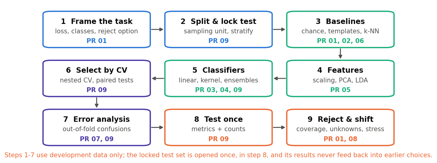
| Step | Question it answers | Main tools | Track chapter |
|---|---|---|---|
| 1 Frame | What is an observation, a class, a mistake? | loss matrix, reject option | PR 01 |
| 2 Split | Which data may inform which decision? | stratified, grouped splits | PR 09 |
| 3 Baselines | What does “good” mean here? | chance, class means, k-NN, naive Bayes | PR 01, 02, 06 |
| 4 Features | What representation do classifiers see? | scaling, PCA, LDA | PR 05 |
| 5 Classifiers | Which model families are plausible? | linear, kernel, ensemble | PR 03, 04, 09 |
| 6 Select | Which configuration, and is the gap real? | nested CV, corrected t-test | PR 09 |
| 7 Analyze | Why does it fail, and would more data help? | out-of-fold confusions, learning curve | PR 07, 09 |
| 8 Test | How well does the frozen procedure do? | accuracy with interval, per-class report | PR 09 |
| 9 Stress | What about doubt, novelty and shift? | coverage–risk, unknown classes, perturbations | PR 01, 08 |
All code below runs on a laptop CPU in well under a minute and uses only scikit-learn’s bundled data [4]. The snippets in steps 2 to 8 form one script: run them in order in the same Python session.
Step 1 — Frame the task
Plain version. Before touching a model, write down what one example is, what the possible answers are, what a mistake costs, and when the system is allowed to say “I don’t know”.
A written protocol
A protocol is a short document you write before experimenting. It protects you from changing the question after seeing the answer. For any recognition project, answer at least these questions:
- Observation. What is one input? An image, a crop, a video clip, a whole document?
- Sampling unit. Which observations share a source (a person, a camera, a patient, a day)? Observations from the same source are not independent and must stay on the same side of every split.
- Label space. Which classes are known during training? What should happen to inputs from other categories?
- Loss. Are all mistakes equally bad? Is abstaining allowed, and what does it cost?
- Data roles. What may training data, validation data and test data each be used for?
- Deployment conditions. Which devices, writers, lighting or time periods must the evaluation cover?
The decision rule we are aiming for
PR 01 showed that under zero–one loss the Bayes classifier picks the class with the largest posterior probability. Adding a reject option with cost (where a correct decision costs 0 and an error costs 1) gives the reject-option rule that Bishop presents in his decision-theory section [2]:
Here is the feature vector, is class , is its posterior probability, and is the cost of rejecting relative to the cost of an error. If , rejecting is free and we reject everything that is not certain; if for classes, we never reject. Everything that follows (classifier choice, validation, threshold setting) is an attempt to approximate this rule with finite data. Keep in mind one limitation: the rule only protects against doubt among known classes. A completely new category can still receive a large posterior, which is why step 9 treats unknowns separately.
Our project and its data card
We will recognize handwritten digits using sklearn.datasets.load_digits [4]. Writing a short “data card” for it is part of the framing (this is the spirit of datasheets for datasets [24]):
- Origin. The data are a copy of the test portion of the UCI “Optical Recognition of Handwritten Digits” dataset by Alpaydin and Kaynak [3].
- Observations. 1,797 images. Each started as a binary bitmap that was divided into non-overlapping blocks; each of the resulting cells counts the “on” pixels, so values are integers from 0 to 16 [3].
- Classes. Ten digits, roughly balanced (174 to 183 images per class).
- Sources. According to the dataset description, this portion was written by 13 people, different from the 30 who wrote the UCI training portion [3]. Writer IDs are not provided.
The last point shapes every claim we can make. Because we cannot group by writer, our random splits place images by the same 13 people on both sides. The test accuracy we report will therefore estimate performance on new images from these writers, not on new writers. The UCI training portion, written by different people, would allow a writer-disjoint test, but it is not bundled with scikit-learn and we do not use it here. Stating this limitation openly is part of an honest result.
Step 2 — Split the data and lock the test set
Plain version. Put a quarter of the data in a “locked drawer” right away. Every decision until step 8 is made without it.
Code · Python · 15 lines
import numpy as np
import warnings
warnings.filterwarnings("ignore", message=".*within_class_std_dev_.*")
from sklearn.datasets import load_digits
from sklearn.model_selection import train_test_split

digits = load_digits()
X, y = digits.data, digits.target          # 1797 x 64, integer intensities 0..16
print("shape:", X.shape, "range:", X.min(), X.max())
print("class counts:", np.bincount(y))

idx = np.arange(len(y))
dev, test = train_test_split(idx, test_size=0.25, stratify=y, random_state=0)
assert not set(dev) & set(test)
print("development:", len(dev), "test (locked):", len(test))
Output: shape: (1797, 64) range: 0.0 16.0, class counts between 174 and 183, development: 1347 test (locked): 450. (The warnings filter only silences a harmless notice that NearestCentroid prints because some border pixels are constant within a class.)
Why stratify? With 450 test images, a random split could easily leave one digit under-represented. Stratification keeps the class proportions the same in both parts. It does not fix dependence between observations; only grouping by the sampling unit does that (PR 09).
Leakage: the most common way to fool yourself
Kapoor and Narayanan surveyed reproducibility failures in machine-learning-based science and found data leakage across many fields; they organize it into a taxonomy that includes no clean train–test separation, preprocessing fitted on all data, duplicates across splits, illegitimate features, and test sets that do not match the population of interest [5]. In a recognition project, the most frequent forms are:
- fitting a scaler, PCA or feature selector on all data before splitting;
- choosing hyperparameters, features or thresholds by looking at test scores;
- near-duplicate images (consecutive video frames, augmented copies, the same person) on both sides of a split;
- a test set from a different population than the deployment (for example, one writer group when deployment involves new writers).
The remedy is structural: keep every fitted transformation inside a scikit-learn Pipeline, so cross-validation refits it on each training fold, and keep the test indices out of every function call until step 8.
Step 3 — Look at the data and set baselines
Plain version. Before training anything clever, look at examples and compute what simple methods achieve. A fancy model that barely beats a trivial one is not a success.
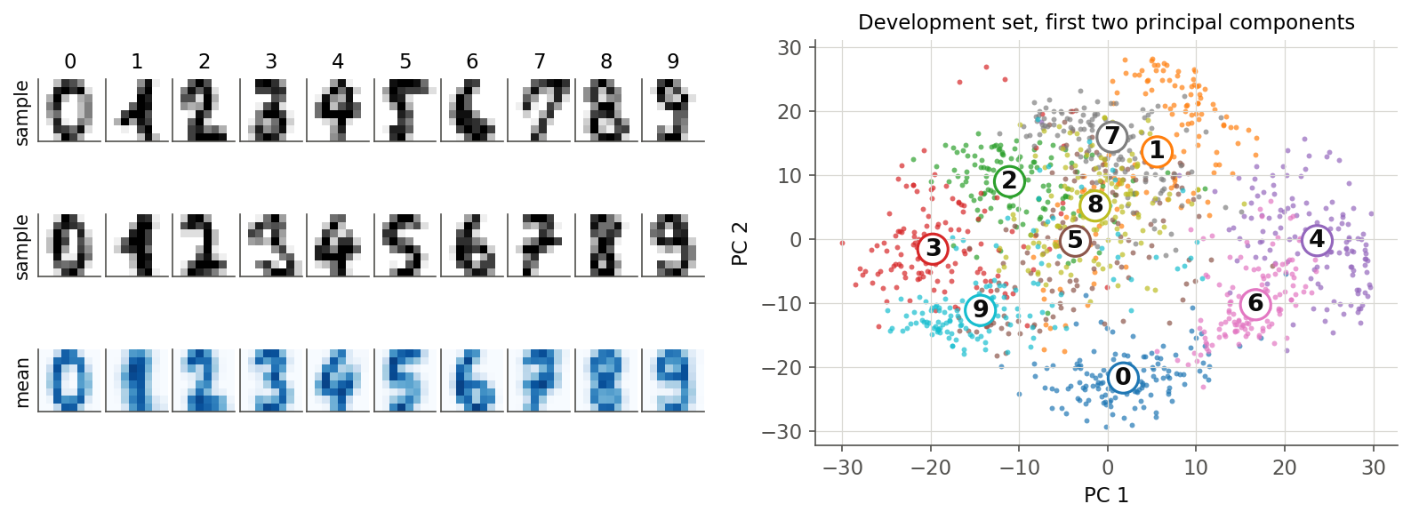
Figure 2 already suggests the difficulty structure. The class means look like clean digits, so template matching (PR 06) should work reasonably. In two principal components, some classes are well separated and others overlap; PR 05 explained why high-variance directions need not be the most discriminative, so overlap in two components says little about overlap in 64 dimensions.
We use four baselines, each tied to a chapter:
- Majority class. Always predict the most common digit. With ten balanced classes this gives about 10% accuracy. It is the floor.
- Nearest class mean. Compare an image with each class mean and pick the closest: the simplest template matcher.
- Gaussian naive Bayes. A Bayes classifier (PR 01) with class-conditional Gaussian densities whose covariance is diagonal. Pixels are strongly correlated, so the independence assumption is badly wrong here, and we expect it to suffer.
- k-nearest neighbors. A nonparametric density-based rule (PR 02): vote among the closest training images.
Step 4 — Decide on features
Plain version. A classifier only sees numbers. Decide which numbers, how they are scaled, and whether to compress them, and fit any of those transformations on training folds only.
Our raw features are the 64 block counts. Three common transformations are worth comparing:
Standardization. Subtract each feature’s training mean and divide by its standard deviation:
where is pixel , and are its mean and standard deviation over the training fold, and is the standardized value. This matters for distance-based and gradient-based methods when features have very different units. Here all features already share the same unit (a count from 0 to 16). Worse, the border pixels are almost always 0, so their is tiny: standardizing them amplifies rare stray strokes into large values. We will see that this choice measurably hurts the kernel SVM.
Principal component analysis. PCA projects onto the directions of largest variance (PR 05). With components the representation is , where holds the top eigenvectors of the training covariance. It removes noise directions and speeds up kernels, but variance is not the same as class information.
Linear discriminant analysis. LDA (PR 03, PR 05) finds at most directions that maximize between-class over within-class scatter. We use it as a classifier with shrinkage, which regularizes the within-class covariance estimate.
For real images, this is also where you would add engineered features (HOG, LBP, moments, see the feature extraction chapter) or pretrained embeddings. At resolution, the raw counts are a reasonable starting representation.
Step 5 — Compare candidate classifiers
Plain version. Run every candidate through the same cross-validation splits of the development set and compare their score distributions, not just their best fold.
Code · Python · 33 lines
from sklearn.model_selection import RepeatedStratifiedKFold, cross_val_score
from sklearn.pipeline import make_pipeline
from sklearn.preprocessing import StandardScaler
from sklearn.decomposition import PCA
from sklearn.dummy import DummyClassifier
from sklearn.neighbors import NearestCentroid, KNeighborsClassifier
from sklearn.naive_bayes import GaussianNB
from sklearn.discriminant_analysis import LinearDiscriminantAnalysis
from sklearn.linear_model import LogisticRegression
from sklearn.svm import SVC
from sklearn.ensemble import RandomForestClassifier

candidates = {
    "majority class (PR 01)": DummyClassifier(strategy="most_frequent"),
    "nearest class mean (PR 06)": NearestCentroid(),
    "Gaussian naive Bayes (PR 01)": GaussianNB(),
    "k-NN, k=3 (PR 02)": KNeighborsClassifier(n_neighbors=3),
    "LDA, shrinkage (PR 03/05)": LinearDiscriminantAnalysis(
        solver="lsqr", shrinkage="auto"),
    "logistic regression (PR 03)": make_pipeline(
        StandardScaler(), LogisticRegression(C=1.0, max_iter=3000)),
    "PCA-30 + RBF SVM (PR 04/05)": make_pipeline(
        StandardScaler(), PCA(n_components=30, random_state=0),
        SVC(C=10, gamma="scale")),
    "random forest (PR 09)": RandomForestClassifier(
        n_estimators=300, random_state=0, n_jobs=1),
}
cv = RepeatedStratifiedKFold(n_splits=5, n_repeats=2, random_state=0)
cv_scores = {}
for name, model in candidates.items():
    s = cross_val_score(model, X[dev], y[dev], cv=cv, scoring="accuracy")
    cv_scores[name] = s
    print(f"{name:30s} {s.mean():.3f} +/- {s.std():.3f}")
Output (mean ± standard deviation over the 10 folds):
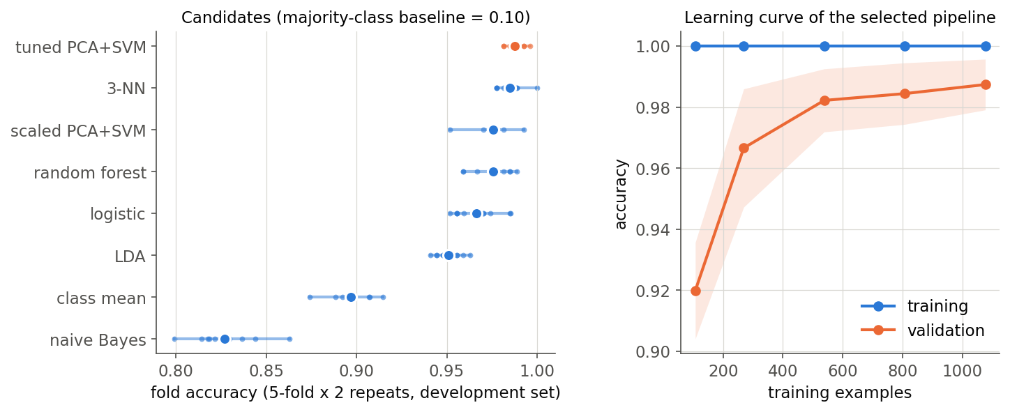
| Candidate | Mean CV accuracy | Std |
|---|---|---|
| majority class | 0.100 | 0.000 |
| Gaussian naive Bayes | 0.827 | 0.017 |
| nearest class mean | 0.897 | 0.011 |
| LDA with shrinkage | 0.951 | 0.007 |
| logistic regression (scaled) | 0.966 | 0.012 |
| random forest, 300 trees | 0.975 | 0.010 |
| scaled PCA-30 + RBF SVM | 0.976 | 0.010 |
| 3-nearest neighbors | 0.985 | 0.007 |
Several lessons are already visible:
- The ranking of simple models follows their assumptions. Naive Bayes, whose independence assumption is violated by correlated neighboring pixels, is the weakest real model. A single template per class (nearest mean) cannot capture different writing styles of the same digit. LDA, which models a shared full covariance, does much better.
- The best untuned model is the simplest nonparametric one. 3-NN beats every untuned parametric model. With 1,347 small images and only 13 writers, many test images have a near twin in the training folds, which is exactly the situation where nearest neighbors shine. This also reminds us that our split measures “new images from known writers”.
- Defaults are not a fair comparison. The SVM and the logistic regression ran with a standardization step and default-ish settings. Before concluding anything, the strong candidates deserve tuning, under a protocol that does not bias the comparison.
Step 6 — Tune and select without fooling yourself
Plain version. Tuning is part of the method. To estimate how good “SVM with tuning” is, you must repeat the whole tuning inside each outer fold. Then ask whether the remaining gap to the next-best model is bigger than the noise.
Nested cross-validation
The inner loop chooses hyperparameters; the outer loop scores the whole procedure. If you report the best inner score directly, you report the maximum of many noisy numbers, which is optimistically biased. Varma and Simon showed this bias empirically for cross-validated model selection [6], and Cawley and Talbot showed that over-fitting the model-selection criterion can produce performance differences as large as the differences between learning algorithms [7]. Raschka’s tutorial review collects the practical recipes [9].
Code · Python · 17 lines
from sklearn.model_selection import GridSearchCV, StratifiedKFold
from sklearn.pipeline import Pipeline

svm = Pipeline([("scale", StandardScaler()), ("pca", PCA(random_state=0)),
                ("svc", SVC())])
grid = {"scale": [StandardScaler(), "passthrough"],
        "pca": [PCA(30, random_state=0), "passthrough"],
        "svc__C": [1, 10],
        "svc__gamma": ["scale", 0.001]}
inner = StratifiedKFold(5, shuffle=True, random_state=1)
outer = StratifiedKFold(5, shuffle=True, random_state=2)
search = GridSearchCV(svm, grid, cv=inner, scoring="accuracy")
nested = cross_val_score(search, X[dev], y[dev], cv=outer)
print("nested-CV accuracy of the tuning procedure:",
      nested.round(3), "mean", nested.mean().round(3))
search.fit(X[dev], y[dev])
print("chosen on all development data:", search.best_params_)
Output: outer-fold accuracies [0.993 0.993 0.985 0.985 0.993], mean 0.99. The configuration chosen on all development data is no standardization, PCA with 30 components, , .
Two observations. First, the grid includes the preprocessing decision itself ("passthrough" means “skip this step”), and validation rejected standardization, confirming the argument of step 4. Second, the nested estimate (0.990) describes the procedure “run this grid search, then refit”, which is what we will deploy. It is not a property of one particular hyperparameter setting.
Is the winner really better?
The tuned SVM (0.990 nested) and 3-NN (0.985) differ by half a percentage point. Is that real? A naive paired t-test on fold scores treats the folds as independent samples, but the training sets of different folds overlap heavily, so the fold scores are positively correlated and the naive test is too confident. Nadeau and Bengio proposed a corrected variance for resampled designs [8]:
where is the score difference between the two models on resample , and are the mean and sample variance of the differences, and and are the training and test sizes of each resample. The extra term inflates the variance to account for overlap. The statistic is compared with a distribution with degrees of freedom. PR 09 derives this and discusses alternatives such as McNemar’s test.
Code · Python · 16 lines
from scipy import stats

def corrected_t(a, b, n_train, n_test):
    """Nadeau-Bengio corrected resampled t-test on paired fold scores."""
    d = np.asarray(a) - np.asarray(b)
    k = len(d)
    var = d.var(ddof=1) * (1 / k + n_test / n_train)
    t = d.mean() / np.sqrt(var)
    return t, 2 * stats.t.sf(abs(t), df=k - 1)

n_test_fold = len(dev) // 5
tuned = cross_val_score(search.best_estimator_, X[dev], y[dev], cv=cv)
t, p = corrected_t(tuned,
                   cv_scores["k-NN, k=3 (PR 02)"],
                   n_train=len(dev) - n_test_fold, n_test=n_test_fold)
print(f"tuned SVM vs k-NN: corrected t = {t:.2f}, p = {p:.3f}")
Output: tuned SVM vs k-NN: corrected t = 1.03, p = 0.331.
Treat this output as an exploratory illustration of variance correction, not a confirmatory significance test. The SVM configuration was selected using all development labels before these repeated folds were made; the correction addresses overlapping folds, not that selection bias [7, 8]. A nonsignificant number also does not prove equivalence. For a fresh comparison, run cross_val_score(search, ...) so tuning is repeated inside every evaluation fold, evaluate the predeclared comparator on the same outer splits, and state the remaining approximation in the statistical test. Here we retain 3-NN as a strong alternative and proceed with the tuned SVM based on the earlier nested evaluation and practical storage/prediction requirements, without claiming a statistically established tie.
Step 7 — Error analysis on development data
Plain version. Look at the mistakes, but look at development mistakes. Once you start redesigning the system because of test errors, the test set stops being a test.
Out-of-fold predictions
cross_val_predict returns, for each development image, the prediction of a model that did not train on it. These predictions are useful for development error analysis. However, chosen was selected using all development labels: each image was excluded from coefficient fitting, not from hyperparameter selection. Do not report this error count as an unbiased evaluation of tuning; pass the full search into the outer prediction loop when that is the goal [7].
Code · Python · 15 lines
from sklearn.model_selection import cross_val_predict
from sklearn.metrics import confusion_matrix

chosen = search.best_estimator_
oof = cross_val_predict(chosen, X[dev], y[dev],
                        cv=StratifiedKFold(5, shuffle=True, random_state=3))
cm_dev = confusion_matrix(y[dev], oof)
off = cm_dev.copy()
np.fill_diagonal(off, 0)
order = np.argsort(off.ravel())[::-1][:5]
print("out-of-fold errors:", int(off.sum()), "of", len(dev))
for t_, p_ in zip(*np.unravel_index(order, off.shape)):
    print(f"  true {t_} -> predicted {p_}: {off[t_, p_]}")
dev_errors = dev[oof != y[dev]]
print("first misclassified dataset indices:", dev_errors[:8])
Output: 17 errors out of 1,347. The most frequent confusions are 9 → 8 (3 times), 5 → 9 (3), 8 → 1 (2), then single errors such as 9 → 5 and 6 → 8.
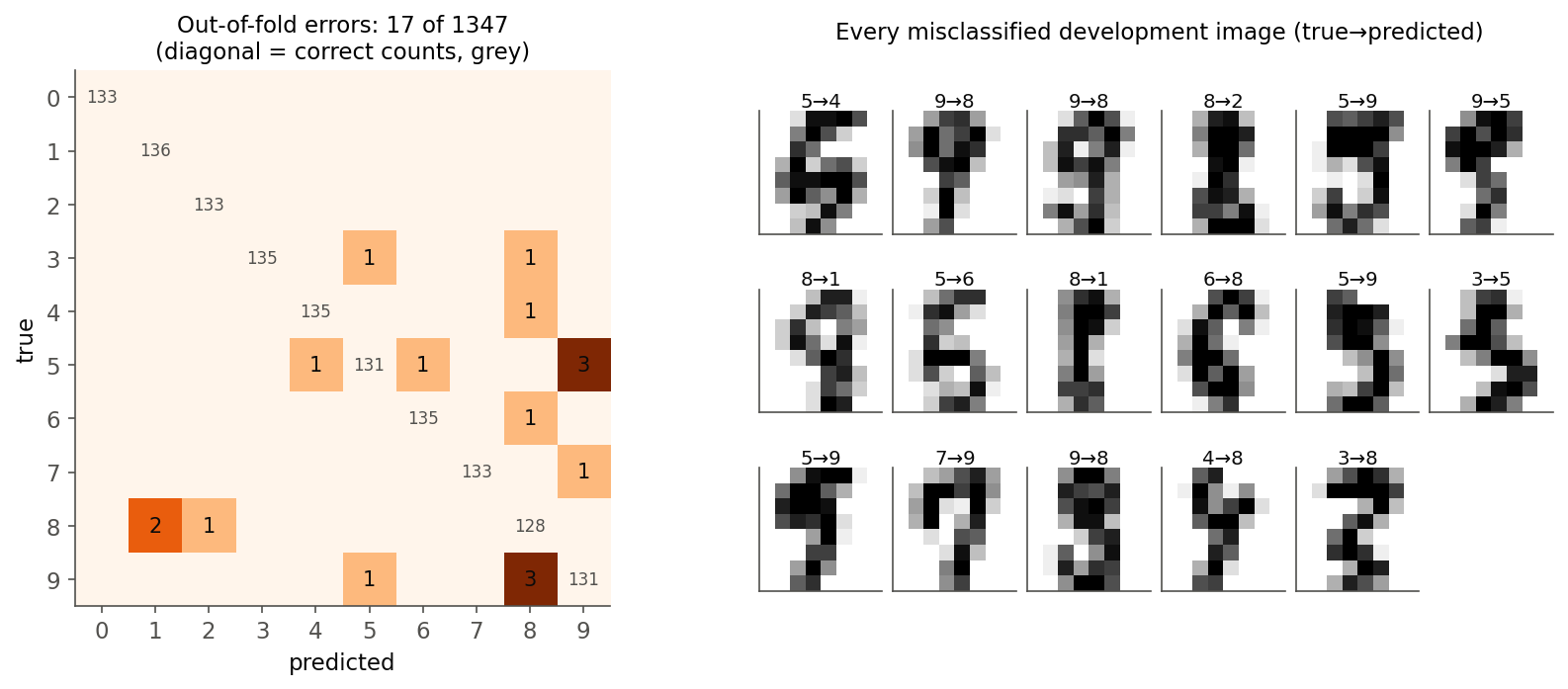
Reading Figure 4 is where domain knowledge enters:
- Systematic confusions. The errors are concentrated among digits with closed upper loops (5, 8, 9) and thin vertical strokes (1, 8). At resolution, the gap that distinguishes a 9 from an 8 may be a single cell.
- Label or quality issues. Some misclassified images are ambiguous even to a human. In a larger project you would review such cases and decide whether they are labeling errors (to fix), genuinely ambiguous inputs (candidates for rejection, step 9), or ordinary failures (to address with features or data).
- Grouping errors. With hundreds of errors you cannot inspect them one by one. A common trick is to cluster the misclassified examples in a feature space (PR 07) and inspect a few members of each cluster; clusters often correspond to one failure mode, such as a writing style or an acquisition problem.
A good error analysis ends with hypotheses, each paired with an experiment that can be run on development data: “a one-pixel shift invariance might help 5/9 confusions; try augmenting training folds with shifted copies and re-run the nested comparison.”
Would more data help? The learning curve
Code · Python · 7 lines
from sklearn.model_selection import learning_curve

sizes, tr, va = learning_curve(
    chosen, X[dev], y[dev], cv=StratifiedKFold(5, shuffle=True, random_state=3),
    train_sizes=[0.1, 0.25, 0.5, 0.75, 1.0])
for n, a, b in zip(sizes, tr.mean(1), va.mean(1)):
print(f"n={n:4d} train={a:.3f} validation={b:.3f}")| Training images | Training accuracy | Validation accuracy |
|---|---|---|
| 107 | 1.000 | 0.920 |
| 269 | 1.000 | 0.967 |
| 538 | 1.000 | 0.982 |
| 807 | 1.000 | 0.984 |
| 1,077 | 1.000 | 0.987 |
The training accuracy is perfect at every size, and the validation accuracy is still rising slowly at the right edge (Figure 3, right). In bias–variance terms (PR 09) the remaining error is mostly variance: the model is flexible enough, and more (or more varied) training data would likely help a little. Had both curves plateaued together at a low value, the advice would be the opposite: a more expressive model or better features.
Step 8 — Open the test set, once
Plain version. Freeze every choice, run the final pipeline on the locked test images, and report the result with its uncertainty and its limits.
Code · Python · 17 lines
from sklearn.metrics import (accuracy_score, balanced_accuracy_score,
                             classification_report)

final = search.best_estimator_            # already refit on all of dev
pred = final.predict(X[test])
print("TEST accuracy:", round(accuracy_score(y[test], pred), 4),
      "balanced:", round(balanced_accuracy_score(y[test], pred), 4),
      "errors:", int((pred != y[test]).sum()), "of", len(test))
cm = confusion_matrix(y[test], pred)
print(cm)
print(classification_report(y[test], pred, digits=3))

k, n, z = int((pred == y[test]).sum()), len(test), 1.96   # Wilson interval
phat = k / n
centre = (phat + z**2 / (2 * n)) / (1 + z**2 / n)
half = z * np.sqrt(phat * (1 - phat) / n + z**2 / (4 * n**2)) / (1 + z**2 / n)
print(f"95% Wilson interval for accuracy: [{centre - half:.3f}, {centre + half:.3f}]")
Output: test accuracy 0.9933 (3 errors out of 450: one each of 3 → 7, 8 → 1 and 9 → 5), balanced accuracy 0.9933, per-class recall between 0.977 and 1.000, and a 95% Wilson interval of [0.981, 0.998].
How to read and report this:
- Report counts, not just percentages. “3 errors out of 450” tells the reader immediately how much the third decimal can be trusted.
- Report an interval. For an accuracy close to 1, the usual normal approximation can exceed 1 and is unreliable; the Wilson score interval used above stays inside and behaves better near the boundary. With test examples, correct and , its center is with for 95% coverage.
- Compare with the development estimate. The test result (0.993) is consistent with the nested estimate (0.990). If it had been much lower, the likely causes would be leakage in development or a test population that differs from development, and either deserves investigation, but a fix would then need a new untouched test set.
- State the scope. This is accuracy on new images from the same 13 writers (step 1). It is not evidence about new writers, scanners or preprocessing.
The protocol note in the code matters: search.best_estimator_ was refit on all development data once, before testing. Refitting again on development plus test and then reporting the test score would be meaningless. For deployment you may refit the frozen procedure on all labeled data, but the reported number must come from the run above.
Step 9 — Beyond closed-set accuracy
A recognizer that is 99% accurate on a balanced test of known digits can still be useless if it confidently labels a letter as a digit, or collapses when the scanner shifts the image. This step tests three questions the closed-set number cannot answer.
Four tasks that are easy to confuse
| Task | What the system must do | What the evaluation must contain |
|---|---|---|
| Closed-set classification | choose among trained classes | independent examples of known classes |
| Selective classification | abstain on difficult known examples | coverage and error on accepted known examples |
| Open-set recognition | classify known classes and reject unknown categories | held-out categories as well as known examples |
| Anomaly detection | flag deviations from a reference population | a defined normal population and relevant deviations |
A low-confidence known example is not necessarily an unknown category; an unfamiliar category can receive a high confidence; and a valid known object photographed badly may be rejected. These tasks need different data and different metrics.
Selective classification: coverage and risk
Plain version. Let the classifier skip the inputs it is least sure about and measure two things: how many inputs it still answers, and how often those answers are wrong.
For a confidence score and an acceptance threshold , over known-class test examples with predictions and labels :
Here is 1 when its condition holds and 0 otherwise. Selective risk is undefined when nothing is accepted. Plotting risk against coverage while sweeping gives the risk–coverage curve; Geifman and El-Yaniv showed how to choose a threshold for deep networks that guarantees a desired risk with high probability [11]. A useful threshold must be chosen on validation data and then only reported on test data.
Open-set recognition: held-out categories
Plain version. Pretend some digits do not exist during training, then check whether the system rejects them when they show up.
Scheirer and colleagues formalized open-set recognition: a classifier must limit the “open space” it labels as known, because a model trained on classes will otherwise assign every input on Earth to one of them [13]. The simplest baseline score is the maximum softmax (or class) probability, proposed by Hendrycks and Gimpel for detecting misclassified and out-of-distribution examples [12].
We redo the experiment with a reduced label space. Digits 0–5 are known; digits 6–7 are proxy unknowns that development may look at; digits 8–9 are test unknowns reserved for the final evaluation. Validation chooses between two predefined pipelines, and the rejection threshold is the 5th percentile of validation confidences, which targets roughly 95% acceptance of known digits. All choices are frozen before the final block. This script is self-contained.
This is a separate six-class experiment. Its variables live inside open_set_demo() so the original ten-class model, development indices and locked test indices remain unchanged for the later stress tests.
Code · Python · 62 lines
def open_set_demo():
    import numpy as np
    from sklearn.datasets import load_digits
    from sklearn.model_selection import train_test_split
    from sklearn.pipeline import make_pipeline
    from sklearn.preprocessing import StandardScaler
    from sklearn.decomposition import PCA
    from sklearn.linear_model import LogisticRegression
    from sklearn.svm import SVC
    from sklearn.metrics import balanced_accuracy_score, confusion_matrix, roc_auc_score

    digits = load_digits()
    X, y = digits.data, digits.target
    known = np.flatnonzero(y < 6)
    train, rest = train_test_split(known, test_size=0.4,
                                  stratify=y[known], random_state=10)
    valid, test = train_test_split(rest, test_size=0.5,
                                  stratify=y[rest], random_state=10)
    proxy_unknown = np.flatnonzero((y == 6) | (y == 7))
    test_unknown = np.flatnonzero(y >= 8)
    assert not set(train) & (set(valid) | set(test))
    assert not set(proxy_unknown) & set(test_unknown)

    candidates = {
        "linear": make_pipeline(
            StandardScaler(), LogisticRegression(C=1.0, max_iter=1500)),
        "PCA + RBF": make_pipeline(
            StandardScaler(), PCA(n_components=24, random_state=10),
            SVC(C=4.0, gamma=0.02, probability=True, random_state=10)),
    }
    scores = {}
    for name, model in candidates.items():
        model.fit(X[train], y[train])
        validation_p = model.predict_proba(X[valid])
        validation_pred = model.classes_[validation_p.argmax(axis=1)]
        scores[name] = balanced_accuracy_score(y[valid], validation_pred)
    name = max(scores, key=scores.get)
    model = candidates[name]
    threshold = np.quantile(model.predict_proba(X[valid]).max(axis=1), 0.05)
    proxy_conf = model.predict_proba(X[proxy_unknown]).max(axis=1)
    print("Validation candidates:", scores, "selected:", name)
    print("Fixed threshold:", threshold)
    print("Proxy-unknown acceptance:", np.mean(proxy_conf >= threshold))

    # Final evaluation begins here; do not revise choices from these results.
    known_p = model.predict_proba(X[test])
    known_conf = known_p.max(axis=1)
    known_pred = model.classes_[known_p.argmax(axis=1)]
    accept = known_conf >= threshold
    unknown_conf = model.predict_proba(X[test_unknown]).max(axis=1)
    print("Known test balanced accuracy:",
          balanced_accuracy_score(y[test], known_pred))
    print("Known coverage:", accept.mean())
    print("Accepted known accuracy:",
          np.mean(known_pred[accept] == y[test][accept]) if accept.any() else np.nan)
    print("Unknown-test acceptance:", np.mean(unknown_conf >= threshold))
    is_unknown = np.r_[np.zeros(len(test)), np.ones(len(test_unknown))]
    unknown_score = 1 - np.r_[known_conf, unknown_conf]
    print("Unknown detection AUROC:", roc_auc_score(is_unknown, unknown_score))
    print("Known-class confusion matrix:\n", confusion_matrix(y[test], known_pred))

open_set_demo()
Output, in the order printed: validation balanced accuracy 0.982 (linear) versus 0.995 (PCA + RBF), so the RBF pipeline is selected; threshold 0.741; proxy-unknown acceptance 0.083; known test balanced accuracy 0.981; known coverage 0.949; accepted known accuracy 0.995; unknown-test acceptance 0.350; unknown-detection AUROC 0.944.
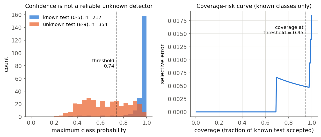
The numbers carry the main lesson of open-set evaluation:
- On known digits, rejection works as intended: 95% coverage and 99.5% accuracy on what is accepted.
- The proxy unknowns (6 and 7) were rejected 92% of the time, which might have suggested that confidence thresholding “solves” unknowns.
- The real test unknowns (8 and 9) were accepted 35% of the time. An 8 looks like a 3 or a 5 with extra strokes, and a 9 looks like a 5 or a 3; the classifier confidently maps them onto those known digits.
- AUROC of 0.944 summarizes ranking over these particular unknowns. It does not fix an operating threshold and does not describe other kinds of novelty.
Performance on one set of proxy unknowns does not transfer to other unknowns. Report which categories were held out, and never claim rejection of “all unfamiliar inputs”. Vaze and colleagues found that a stronger closed-set classifier tends to be a better open-set recognizer, with closed-set and open-set performance strongly correlated across methods [16], so improving the base model and using better scores (feature distances, energy or logit-based scores) are complementary.
Other families of scores model the reference population directly: a one-class SVM estimates a region that contains most of the training data [17], and an Isolation Forest flags points that random axis-aligned splits isolate quickly [18]. An “outlier” may be an acquisition error, a rare valid case or a new class; statistical unusualness does not tell you which.
Distribution shift and stress tests
Plain version. The world changes after you deploy. Ask “what if” questions with controlled perturbations and, better, with real data from new conditions.
Let and be the joint distributions of features and labels during training and deployment. Moreno-Torres and colleagues organized the vocabulary of dataset shift in classification [19]. Three cases matter most:
- Prior (label) shift: class frequencies change, while stays the same. Example: one digit becomes much more common in a new form layout.
- Covariate shift: changes, while stays the same. Example: a new scanner makes strokes thicker.
- Concept shift: itself changes. Example: a new convention for writing 7 with a bar.
These are modeling assumptions, not diagnoses you can read off the data’s name. A camera change can alter class-conditional features; adding a new class breaks the label space entirely.
We cannot collect new handwriting here, but we can probe sensitivity with controlled perturbations of the test images. The model is not retrained; the perturbations were decided before looking at their results.
Code · Python · 16 lines
rng = np.random.default_rng(0)
def shift_right(X, k=1):
    imgs = X.reshape(-1, 8, 8)
    out = np.zeros_like(imgs)
    out[:, :, k:] = imgs[:, :, :-k]
    return out.reshape(len(X), 64)

conditions = {
    "clean": X[test],
    "noise sd=2": np.clip(X[test] + rng.normal(0, 2, X[test].shape), 0, 16),
    "noise sd=4": np.clip(X[test] + rng.normal(0, 4, X[test].shape), 0, 16),
    "shift 1 px right": shift_right(X[test], 1),
    "contrast x0.5": X[test] * 0.5,
}
for name, Xc in conditions.items():
    print(f"{name:18s} accuracy = {accuracy_score(y[test], final.predict(Xc)):.3f}")
(Run this after the step 8 block, not after the open-set script, because it uses the 10-class X, test and final.)
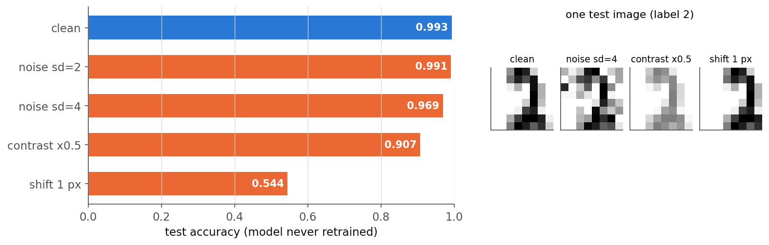
| Condition | Test accuracy |
|---|---|
| clean | 0.993 |
| additive noise, sd = 2 | 0.991 |
| additive noise, sd = 4 | 0.969 |
| contrast halved | 0.907 |
| shifted right by one cell | 0.544 |
Additive noise barely matters. Halving the contrast costs about 9 points, because the RBF kernel compares raw intensities and was tuned for full-contrast strokes. A one-cell translation cuts accuracy almost in half: a pixel-vector classifier has no notion that a shifted 3 is still a 3. One cell corresponds to a 4-pixel block of the original bitmap, an eighth of the image width, so this is a realistic misalignment for a sloppy crop. This is the classic argument for building translation tolerance into the model, by augmentation or by convolution and pooling, which LeCun and colleagues demonstrated for document recognition [10] (see ML 03).
Synthetic perturbations are a cheap first check, not a substitute for real new-condition data. Benchmarks such as WILDS collect real distribution shifts across hospitals, cameras and regions and show sizable drops from in-distribution to out-of-distribution performance [21]; Recht and colleagues rebuilt the CIFAR-10 and ImageNet test sets following the original procedures and observed accuracy drops for many models, even without any deliberate shift [20]. Report results per meaningful condition (writer, device, site, time), not just pooled.
Probabilities that mean what they say
If downstream users act on confidence values, they must be calibrated: among predictions made with confidence 0.8, about 80% should be correct. Guo and colleagues showed that modern deep networks are often overconfident and that a single scalar temperature fitted on validation data is a strong fix [22]. For SVMs, SVC(probability=True) fits Platt scaling internally with cross-validation; CalibratedClassifierCV gives explicit control. Calibration must be fitted on data not used for training the base model, and it does not repair distribution shift.
Bridge to learned and foundation features
Plain version. Swap the hand-made features for a pretrained network’s features. Everything else in this chapter stays the same.
Replace the feature map with a pretrained encoder:
where is the raw image, is a frozen network (for example a self-supervised vision transformer such as DINOv2 [25]), is its embedding, and is a classifier with parameters trained on your labels. A linear probe (logistic regression on frozen embeddings) is the standard baseline; compare it with k-NN on embeddings, a regularized nonlinear head and fine-tuning, holding splits and metrics fixed. ML 06 explains how such features are learned and ML 10 how they are adapted.
The protocol extends naturally:
- record the checkpoint, input resizing, normalization, pooling and embedding dimension;
- fit downstream preprocessing (scaling, PCA) only on training embeddings;
- count the choice of checkpoint, prompt or layer as model selection, made on validation data;
- if evaluation images could have appeared in the pretraining data, state what evidence you have about overlap;
- distance-based unknown scores (k-NN distance to training embeddings) often work much better on good embeddings than on raw pixels, but they still need held-out unknown categories to evaluate.
Representation learning changes how measurements are obtained. It does not change minimum-risk decisions, honest validation or the separation of known-class accuracy from rejection and shift, which is the framework of this track [1], [2].
What to submit
A finished recognition project should include, at minimum:
- Task definition: observation, label space, loss, reject policy.
- Data card: provenance, licensing, sampling unit, class counts, known limitations (here: 13 writers, no writer IDs) [24].
- Split description: what each split was used for, the unit of splitting, seeds.
- Baselines and candidates: all models tried, not just the winner, with development scores and their variability.
- Selection evidence: nested estimate of the chosen procedure and a statistical comparison with the runner-up.
- Error analysis: confusion structure, examples, hypotheses, learning curve.
- Final test result: counts, interval, per-class results, scope statement.
- Stress results: rejection (coverage and risk), held-out unknown categories, shift or perturbation tests, calibration if probabilities are used.
- Reproducibility: environment and library versions, the full pipeline object, class ordering, runtime and memory if they matter.
Model cards formalize the deployment-facing part of this list (intended use, evaluation conditions, performance across relevant groups, caveats) [23]. If the original test set informed any redesign, the revised system needs a new protected test.
Modern view
The capstone workflow is old in its principles and still evolving in practice. The following reviews and studies are good entry points.
Raschka, “Model evaluation, model selection, and algorithm selection in machine learning” (2018) [9]. A long tutorial review that organizes evaluation into three distinct goals: estimating generalization performance, selecting hyperparameters and models, and comparing algorithms. It covers holdout, bootstrap and cross-validation, nested cross-validation and statistical tests (McNemar, 5×2cv and related tests), with practical recommendations by dataset size. It is the closest single reference to steps 2 and 6 of this chapter.
Kapoor and Narayanan, “Leakage and the reproducibility crisis in machine-learning-based science” (Patterns, 2023) [5]. Collects published leakage failures across many scientific fields and proposes a taxonomy of leakage types together with “model info sheets” that ask authors to justify the absence of each type. Its main takeaway is that leakage is common, often invisible in the reported numbers, and best prevented by protocol rather than detected afterwards.
Geng, Huang and Chen, “Recent advances in open set recognition: a survey” (TPAMI, 2021) [14]. Distinguishes known known, known unknown, unknown known and unknown unknown classes and organizes open-set methods into discriminative (traditional ML and deep network based) and generative (instance and non-instance generation) families. It also relates open-set recognition to zero-shot, one-shot and classification-with-reject settings and reviews the datasets and evaluation criteria in use.
Yang, Zhou, Li and Liu, “Generalized out-of-distribution detection: a survey” (IJCV, 2024) [15]. Unifies anomaly detection, novelty detection, open-set recognition, out-of-distribution detection and outlier detection in one framework, distinguishing them by whether shift is semantic or covariate and by what the in-distribution task is. This is the vocabulary to use when deciding which of the “four tasks” table rows your project belongs to.
Vaze, Han, Vedaldi and Zisserman, “Open-set recognition: a good closed-set classifier is all you need?” (ICLR, 2022) [16]. Shows a strong correlation between closed-set accuracy and open-set performance and that a well-trained baseline with a maximum-logit score is competitive with specialized methods; it also proposes the “Semantic Shift Benchmark” to separate semantic novelty from low-level shift.
Koh et al., “WILDS” (ICML, 2021) [21] and Recht et al. (ICML, 2019) [20]. Two complementary views of evaluation under shift: WILDS curates real deployment shifts across domains, while Recht et al. show that even a careful re-collection of a test set “from the same distribution” can lower accuracy. Together they argue for reporting results per condition and treating a single i.i.d. test score as an upper bound.
Guo et al., “On calibration of modern neural networks” (ICML, 2017) [22] and Geifman and El-Yaniv (NeurIPS, 2017) [11] are the starting points for confidence quality and selective prediction in deep models.
State of the art (2023–2026). In practice, recognition projects increasingly begin from frozen or lightly fine-tuned foundation features (for example DINOv2 [25]) with a linear or k-NN head, and spend the saved effort on data quality, evaluation design and documentation. Out-of-distribution evaluation has moved toward unified benchmarks and the semantic-versus-covariate distinction of [15]. Datasheets [24] and model cards [23] provide ready-made templates for documenting data and models alongside these results.
Open problems.
- Unknown unknowns. Any held-out set of “unknown” categories is a sample; there is no general way to certify rejection of all novel inputs.
- Evaluation under shift. Collecting labeled data for every deployment condition is expensive, and synthetic perturbations do not reliably predict real shifts.
- Pretraining overlap. With web-scale pretraining, it is increasingly hard to guarantee that test images were never seen, which complicates the “locked test” principle.
- Small-sample comparisons. Many applied projects have hundreds, not millions, of labeled examples, where the variance of every estimate in this chapter is large and statistical comparison is essential.
Key takeaways
- Write the protocol first: observation, sampling unit, label space, loss, reject policy and the role of each split. Most evaluation failures are protocol failures.
- Lock the test set before any modeling, keep every fitted transformation inside a pipeline, and treat features and preprocessing as hyperparameters.
- Compare all candidates on identical folds; baselines tell you what “good” means, and on these digits a 3-NN baseline is hard to beat.
- Estimate the tuned procedure with nested cross-validation, and use a corrected resampled test before claiming one model is better.
- Do error analysis on out-of-fold development predictions; use learning curves to decide between more data and a richer model.
- Open the test set once and report counts, an interval and the scope (here: new images from the same 13 writers).
- Closed-set accuracy, selective risk, unknown-class rejection and robustness to shift are different properties: a 99%-accurate digit classifier still accepted 35% of unseen digits and lost almost half its accuracy under a one-cell shift.
Exercises
- Distance-based rejection. In the open-set experiment, replace maximum class probability with the distance from a test image to its nearest training image in the train-fitted PCA space. Choose the threshold with validation known digits only, then report known coverage and unknown acceptance on the test sets. Does it beat confidence thresholding?
Hint
Fit StandardScaler and PCA on X[train] only, then use NearestNeighbors(n_neighbors=1) on the transformed training set. The score is the distance (larger means “more unknown”); set the threshold at the 95th percentile of validation distances so about 95% of known validation digits are accepted. Report both numbers; do not change the threshold after seeing the test results.
- Risk–coverage without cheating. Draw the risk–coverage curve of the 10-class tuned SVM using its decision values as confidence, first with out-of-fold development predictions, then (for reporting only) on the test set. Explain how selective accuracy can improve while useful coverage collapses, and what happens at zero coverage.
Hint
Sort examples by decreasing confidence; at each cut, coverage is the fraction kept and risk is the error rate among them. At very low coverage only a few examples remain, so risk is noisy, and at zero coverage it is undefined. Choose any operating point on the development curve, then read off its test value.
- Fix the shift weakness. Augment each training fold with copies of its images shifted by one cell left, right, up and down. Re-run the nested comparison of step 6 and the stress test of step 9. Which accuracies change, and why must augmentation happen inside the folds?
Hint
Write a small transformer or a custom loop that augments only the training part of each split; augmenting before splitting puts shifted copies of validation images into training, which is leakage. Expect the shifted-test accuracy to rise sharply and clean accuracy to stay similar or change slightly.
- Writer-disjoint evaluation by design. The UCI dataset’s training portion was written by 30 people and its test portion by 13 different people [3]. Design (on paper) an experiment that measures generalization to new writers. Which numbers in this chapter would you expect to change, and which conclusions would you no longer be able to draw from the bundled data alone?
Hint
Train and select on one writer group and test on the other. Expect lower accuracy for k-NN in particular, since its advantage relies on near-duplicates from the same writers. Without writer IDs inside a portion, you still cannot do grouped cross-validation within development, so validation remains writer-mixed.
- Is it significant? Using the 10 fold scores from step 5, apply the corrected resampled t-test to logistic regression versus random forest, and to LDA versus logistic regression. Then compute the naive paired t-test without the term. In which case would the two tests lead to different conclusions?
Hint
With 5-fold CV, , which is much larger than , so the corrected variance is about 3.5 times the naive one and the statistic shrinks by a factor of about . Small but consistent differences are where the conclusions diverge.
- Frozen features versus fine-tuning. Design an experiment comparing a linear probe on frozen pretrained features with full fine-tuning for a real image dataset of your choice. List every decision that could leak test information.
Hint
Include checkpoint and layer choice, image resizing and normalization, augmentation, learning-rate and epoch selection (early stopping), threshold and calibration fitting, prompt design if a vision–language model is used, and possible overlap between pretraining data and your test images.
References
- S. Theodoridis and K. Koutroumbas, Pattern Recognition, 4th ed., Academic Press (Elsevier), 2009; Ch. 1 “Introduction”, Ch. 5–7 on feature selection and generation, Ch. 10 “Supervised Learning: The Epilogue”. doi
- C. M. Bishop, Pattern Recognition and Machine Learning, Springer, 2006; Sec. 1.5 (decision theory and the reject option), Sec. 1.3 (model selection), Ch. 14 (combining models). official page and PDF
- E. Alpaydin and C. Kaynak, “Optical Recognition of Handwritten Digits,” UCI Machine Learning Repository, 1998. doi
- F. Pedregosa et al., “Scikit-learn: Machine learning in Python,” Journal of Machine Learning Research, vol. 12, pp. 2825–2830, 2011. JMLR; dataset loader: load_digits
- S. Kapoor and A. Narayanan, “Leakage and the reproducibility crisis in machine-learning-based science,” Patterns, vol. 4, no. 9, 2023. doi
- S. Varma and R. Simon, “Bias in error estimation when using cross-validation for model selection,” BMC Bioinformatics, vol. 7, 91, 2006. doi
- G. C. Cawley and N. L. C. Talbot, “On over-fitting in model selection and subsequent selection bias in performance evaluation,” Journal of Machine Learning Research, vol. 11, pp. 2079–2107, 2010. JMLR
- C. Nadeau and Y. Bengio, “Inference for the generalization error,” Machine Learning, vol. 52, pp. 239–281, 2003. doi
- S. Raschka, “Model evaluation, model selection, and algorithm selection in machine learning,” arXiv:1811.12808, 2018. arXiv
- Y. LeCun, L. Bottou, Y. Bengio and P. Haffner, “Gradient-based learning applied to document recognition,” Proceedings of the IEEE, vol. 86, no. 11, pp. 2278–2324, 1998. doi
- Y. Geifman and R. El-Yaniv, “Selective classification for deep neural networks,” in Advances in Neural Information Processing Systems 30 (NIPS), 2017. proceedings
- D. Hendrycks and K. Gimpel, “A baseline for detecting misclassified and out-of-distribution examples in neural networks,” in Proc. ICLR, 2017. arXiv
- W. J. Scheirer, A. de Rezende Rocha, A. Sapkota and T. E. Boult, “Toward open set recognition,” IEEE Transactions on Pattern Analysis and Machine Intelligence, vol. 35, no. 7, pp. 1757–1772, 2013. doi
- C. Geng, S.-J. Huang and S. Chen, “Recent advances in open set recognition: A survey,” IEEE Transactions on Pattern Analysis and Machine Intelligence, vol. 43, no. 10, 2021. doi
- J. Yang, K. Zhou, Y. Li and Z. Liu, “Generalized out-of-distribution detection: A survey,” International Journal of Computer Vision, 2024. doi
- S. Vaze, K. Han, A. Vedaldi and A. Zisserman, “Open-set recognition: A good closed-set classifier is all you need?,” in Proc. ICLR, 2022. arXiv
- B. Schölkopf, J. C. Platt, J. Shawe-Taylor, A. J. Smola and R. C. Williamson, “Estimating the support of a high-dimensional distribution,” Neural Computation, vol. 13, no. 7, pp. 1443–1471, 2001. doi
- F. T. Liu, K. M. Ting and Z.-H. Zhou, “Isolation forest,” in Proc. IEEE International Conference on Data Mining (ICDM), 2008. doi
- J. G. Moreno-Torres, T. Raeder, R. Alaiz-Rodríguez, N. V. Chawla and F. Herrera, “A unifying view on dataset shift in classification,” Pattern Recognition, vol. 45, no. 1, pp. 521–530, 2012. doi
- B. Recht, R. Roelofs, L. Schmidt and V. Shankar, “Do ImageNet classifiers generalize to ImageNet?,” in Proc. ICML, PMLR 97, pp. 5389–5400, 2019. PMLR
- P. W. Koh, S. Sagawa, H. Marklund et al., “WILDS: A benchmark of in-the-wild distribution shifts,” in Proc. ICML, PMLR 139, pp. 5637–5664, 2021. PMLR
- C. Guo, G. Pleiss, Y. Sun and K. Q. Weinberger, “On calibration of modern neural networks,” in Proc. ICML, 2017. arXiv
- M. Mitchell, S. Wu, A. Zaldivar, P. Barnes, L. Vasserman, B. Hutchinson, E. Spitzer, I. D. Raji and T. Gebru, “Model cards for model reporting,” in Proc. Conference on Fairness, Accountability, and Transparency (FAT*), 2019. doi
- T. Gebru, J. Morgenstern, B. Vecchione, J. W. Vaughan, H. Wallach, H. Daumé III and K. Crawford, “Datasheets for datasets,” Communications of the ACM, vol. 64, no. 12, 2021. doi
- M. Oquab, T. Darcet, T. Moutakanni et al., “DINOv2: Learning robust visual features without supervision,” arXiv:2304.07193, 2023. arXiv
Check your understanding
This tutorial has 6 exercises. Can you solve them without opening the hints?
Go to the exercises ↑This is the last tutorial in Pattern Recognition. Back to the learning map →