PR 04 · Neighbors, Kernels and Nonlinear Classifiers
Needs: PR 03 · Linear Models for Regression and Classification
Navigate: this page and this track: Navigate: this page and this track
On this page
- What you’ll learn1 min
- The big picture1 min
- Nearest-neighbor classification2 min
- Kernels: the kernel trick and Mercer’s condition4 min
- Support vector machines4 min
- Gaussian processes and relevance vectors2 min
- Radial basis function networks1 min
- Decision trees3 min
- Multilayer perceptrons as nonlinear classifiers2 min
- Choosing among nonlinear classifiers1 min
- Modern view3 min
- Key takeaways1 min
- Exercises3 min
- References
Pattern Recognition
Explore this chapter 1 interactive experiment
Run leave-one-out k-nearest-neighbour classification on the real iris measurements, then change the unit of one feature: no flower moves, yet the neighbours and the accuracy do.
What you’ll learn
- How nearest-neighbor rules produce nonlinear decision regions without fitting any parameters, and why the distance metric matters as much as .
- What the kernel trick is, what makes a function a valid (Mercer) kernel, and how to check it on a finite Gram matrix.
- The soft-margin support vector machine: its primal and dual problems, support vectors, and how the hyperparameters and shape the boundary.
- How Gaussian processes and relevance vector machines reuse kernels with a probabilistic interpretation.
- Three other routes to nonlinearity: radial basis function (RBF) networks, decision trees grown with impurity measures (CART), and multilayer perceptrons.
- How to compare these families fairly, and where they stand in 2026.
The big picture
PR 03 built classifiers whose decision boundary is a straight line, a plane or a hyperplane. Many real problems are not like that. Points inside a ring cannot be separated from points outside it by any straight line. Handwritten “1”s and “7”s overlap in pixel space along curved, twisted regions. We need boundaries that bend.
There are only a few basic ways to make them bend:
- Compare with stored examples. Label a new point by looking at the most similar training points (nearest neighbors).
- Change the representation, then stay linear. Map each input to new features in which a hyperplane does work. Kernels do this implicitly; RBF networks and multilayer perceptrons do it explicitly, with learned or fixed basis functions.
- Cut the space into pieces. A decision tree asks a sequence of yes/no questions, and each answer path ends in a small box with its own label.
One warning applies to every method in this chapter. A nonlinear classifier can only use information that the measurements contain. If two classes look identical in the features you recorded, no amount of boundary-bending will separate them. Feature design is the subject of PR 05. The textbook background for this chapter is Theodoridis and Koutroumbas, Chapters 2 and 4 [1], and Bishop, Sections 2.5.2, 5.1–5.3, 6.1–6.4, 7.1–7.2 and 14.4 [2].
Nearest-neighbor classification
In plain words. To classify a new point, find the training points closest to it and let them vote. Nothing is “learned” beyond storing the data, yet the resulting boundary can follow any shape the data have.
The rule and its guarantee
Given training pairs , , and a query , let be the indices of the training points nearest to under some distance . The -nearest-neighbor (-NN) rule predicts
where runs over the classes, is 1 when its argument is true and 0 otherwise, and is a vote weight: for plain majority voting, or a decreasing function of for distance-weighted voting.
The vote fractions are a crude estimate of the class posteriors : -NN is a nonparametric density method in disguise (PR 02), with the neighborhood size set by rather than by a fixed bandwidth [2]. Cover and Hart proved the classic result for the 1-NN rule: as the number of training samples grows without bound, its error rate is at most twice the Bayes error rate [3]. This is an asymptotic statement. With finite data, especially in high dimension, -NN can be far from that bound.
The metric is a modeling decision
Euclidean distance treats a one-unit difference in every coordinate as equally important. If one feature is measured in millimeters and another in kilometers, the first will dominate every neighborhood. Standardizing features, learning a Mahalanobis metric with a positive semidefinite matrix , or comparing normalized embeddings by cosine similarity all change who counts as a neighbor.
For vectors and normalized to unit length,
So the nearest neighbor by Euclidean distance is exactly the neighbor with the largest cosine similarity: the two criteria rank candidates in reverse order of each other and pick the same neighbors. This is why nearest-neighbor search over normalized deep features (ML 06) can use either.
Choosing , and the cost of prediction
A small (such as 1) gives a jagged boundary that follows every noisy training point: low bias, high variance. A large averages over a wide region and smooths the boundary, but it can wash out a small class entirely. Choose , the metric and the scaling by cross-validation on training data only.
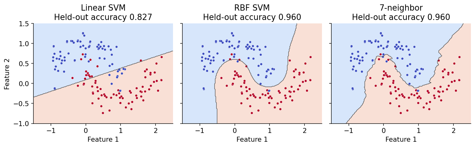
-NN shifts all the cost to prediction time. A naive query compares with all training points, which costs for -dimensional inputs. Tree-based indices and approximate nearest-neighbor search reduce this in practice. In high dimension, a further problem appears: when many coordinates carry irrelevant variation, distances between random points concentrate around a common value, and “nearest” stops meaning “most similar.” The right panel of Figure 3 later in this chapter shows a 7-NN boundary on a two-dimensional toy problem, where none of these problems arise.
Kernels: the kernel trick and Mercer’s condition
In plain words. Many linear algorithms only ever use inputs through inner products . If we replace every inner product by a “similarity function” that equals an inner product in some richer feature space, we get a nonlinear algorithm for the price of a linear one, without ever computing the rich features.
Lifting the data
Take the ring data on the left of Figure 1. No line separates the inner disc from the outer ring. Add a third feature, the squared radius . In the new three-dimensional space the inner points sit low and the outer points sit high, and a flat plane separates them perfectly. A linear classifier in the lifted space is a circle in the original space.
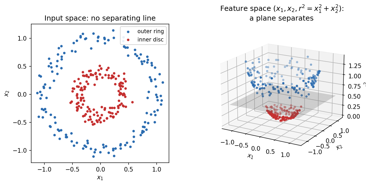
Explicit lifting gets expensive quickly. All monomials of degree up to in variables number ; for a image () and that is about 2.9 million features. Kernels avoid building them.
The kernel trick
A kernel is a function for which there exists a feature map into some inner-product space with
Here and are inputs, is the (possibly very long, even infinite) feature vector of , and the right-hand side is their inner product. For example, in two dimensions, with ,
Evaluating the left side costs one inner product and one square. The right side needs six features per point. For degree in dimensions, the left side still costs .
The kernel trick is the observation that any algorithm written entirely in terms of inner products between data points can be “kernelized” by replacing with [7]. The SVM dual, kernel ridge regression, kernel PCA (PR 05) and Gaussian processes are all of this kind. The result is collected in the Gram matrix , .
The code below checks the identity numerically, and then shows a popular “similarity” that is not a valid kernel.
Code · Python · 18 lines
import numpy as np

rng = np.random.default_rng(0)
x, z = rng.normal(size=2), rng.normal(size=2)

def phi(v):  # explicit feature map of (v.w + 1)^2 in 2-D
    a, b = v
    s = np.sqrt(2)
    return np.array([1, s * a, s * b, a * a, b * b, s * a * b])

lhs = (x @ z + 1) ** 2
rhs = phi(x) @ phi(z)
print("kernel:", round(lhs, 6), " explicit:", round(rhs, 6))
assert np.isclose(lhs, rhs)

X = rng.normal(size=(40, 2))
K_sig = np.tanh(2.0 * X @ X.T - 1.0)        # "sigmoid kernel"
print("sigmoid Gram min eigenvalue:", np.linalg.eigvalsh(K_sig).min().round(3))
The two numbers agree. The “sigmoid kernel” Gram matrix has a clearly negative eigenvalue (about here), so for these parameters no feature map can reproduce it.
Which functions are kernels? Mercer’s condition
A function is a valid kernel exactly when it is symmetric, , and positive semidefinite: for every finite set of points and every real vector ,
Equivalently, every Gram matrix has nonnegative eigenvalues. Symmetry alone is not enough, as the sigmoid example shows.
Mercer’s theorem [4] gives the continuous version. For a continuous symmetric on a compact domain , positive semidefiniteness in the integral sense,
guarantees an expansion with eigenvalues and orthonormal eigenfunctions . The feature map is then . In modern terms, every positive semidefinite kernel defines a reproducing kernel Hilbert space (RKHS) of functions, and the representer theorem says that regularized fits in that space are finite combinations [7].
Valid kernels can be built from valid kernels. If and are kernels, so are , for , , , and for any function [2]. The common kernels follow:
| Kernel | Formula | Parameters | Notes |
|---|---|---|---|
| Linear | none | Recovers the linear model | |
| Polynomial | , , integer | All monomials up to degree (: degree only) | |
| Gaussian RBF | Infinite-dimensional feature space; local similarity | ||
| Laplacian | Rougher functions than the Gaussian | ||
| Sigmoid | Not positive semidefinite in general |
The Gaussian RBF kernel is the default nonlinear choice. Its parameter (sometimes written with a bandwidth ) sets how far similarity reaches. A large makes each training point influence only a tiny neighborhood; a small makes the kernel nearly constant over the data, so the model approaches a very smooth, almost linear function. Because multiplies squared distances, it is tied to the scale of the features: scaling is part of the model. Standardization is a useful default for mixed units, but features already sharing meaningful units may work better without it, as the PR 10 capstone illustrates. Compare these choices inside validation, and fit any scaler only on each training fold [27].
Kernel ridge regression: the trick in one line
Ridge regression with features minimizes . Its solution can be written as , which leads to
where are the targets, is the regularization strength, is the identity, and holds the similarities of a query to the training points. The -dimensional feature-space solve has become an sample-space solve: attractive when features are many and samples few, expensive ( time, memory) when is large.
Code · Python · 16 lines
import numpy as np
from sklearn.kernel_ridge import KernelRidge
from sklearn.metrics.pairwise import rbf_kernel

rng = np.random.default_rng(1)
X = rng.uniform(-3, 3, size=(60, 1))
t = np.sin(X[:, 0]) + 0.1 * rng.normal(size=60)
lam, gamma = 0.1, 0.5

K = rbf_kernel(X, X, gamma=gamma)
alpha = np.linalg.solve(K + lam * np.eye(len(X)), t)
Xq = np.linspace(-3, 3, 5)[:, None]
f_ours = rbf_kernel(Xq, X, gamma=gamma) @ alpha
f_skl = KernelRidge(alpha=lam, kernel="rbf", gamma=gamma).fit(X, t).predict(Xq)
print(np.round(f_ours, 4))
assert np.allclose(f_ours, f_skl)
The hand-written solve and scikit-learn’s KernelRidge agree, and the predictions follow at the five query points.
Support vector machines
In plain words. Among all boundaries that separate the classes, pick the one with the widest empty “street” between them. Only the points on the edges of the street, or inside it, matter; they are the support vectors. Allowing a few points into the street, at a price , makes the method work on overlapping data. Replacing inner products by a kernel makes the street curve.
Hard and soft margins
Use labels and a score , with weight vector and bias ; predict the sign of . If the data are separable, scale and so that the closest points satisfy . The distance between the two lines , the margin, is then . Maximizing it means minimizing subject to for all : the hard-margin SVM of Boser, Guyon and Vapnik [5].
Real data overlap, so Cortes and Vapnik introduced slack variables that measure how far each point violates the margin [6]. The soft-margin SVM solves
A point with is on the correct side with margin at least one. At an optimum, means a point is inside the street but correctly classified; lies on the decision boundary, and is misclassified. The constant sets the price of violations. Eliminating gives the equivalent unconstrained form
regularized hinge loss. A point with contributes no loss at all; this is the source of the SVM’s sparsity. (Some texts average the losses and put the constant on the regularizer instead, writing . The two forms match when .)
The dual problem and support vectors
Introducing a Lagrange multiplier for each margin constraint and eliminating , and gives the dual problem [2], [6]:
It is a convex quadratic program in the multipliers , and the data appear only through kernel values . That is where the kernel trick enters. The optimal weight vector is , so predictions need only kernels too:
The Karush–Kuhn–Tucker (KKT) optimality conditions sort the training points into three groups:
- : the point is outside the street () and has no influence on ;
- : the point lies exactly on the margin (); these points determine ;
- : the point is inside the street or misclassified ().
Points with are the support vectors. Deleting any other point and retraining gives the same classifier. How many there are depends on the data: on a heavily overlapping problem, a large fraction of the training set can end up as support vectors, and prediction becomes as expensive as nearest-neighbor search.
How and shape an RBF-SVM
With the Gaussian kernel, two numbers control everything. sets how much the training errors cost relative to a wide margin; sets how local the kernel is. Figure 2 sweeps both on the same noisy data.
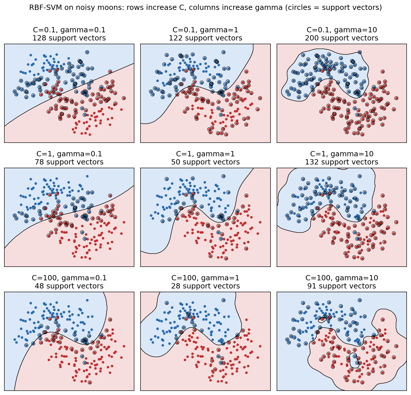
Read the grid like this. Moving down (larger ) makes the boundary chase individual training points, and the number of support vectors drops because fewer points are allowed inside the margin. Moving right (larger ) shrinks each point’s sphere of influence; at the classifier draws little islands, which is overfitting. The good region is a diagonal band: when grows, a smaller is usually needed. In practice one searches and on a logarithmic grid with cross-validation.
Code · Python · 30 lines
import numpy as np
from sklearn.datasets import make_moons
from sklearn.model_selection import GridSearchCV, train_test_split
from sklearn.neighbors import KNeighborsClassifier
from sklearn.pipeline import make_pipeline
from sklearn.preprocessing import StandardScaler
from sklearn.svm import SVC

X, y = make_moons(n_samples=500, noise=0.18, random_state=2)
Xtr, Xte, ytr, yte = train_test_split(
    X, y, test_size=0.3, stratify=y, random_state=2)
models = {
    "linear SVM": SVC(kernel="linear", C=1),
    "RBF SVM": SVC(kernel="rbf", C=3, gamma=0.7),
    "7-neighbor": KNeighborsClassifier(n_neighbors=7),
}
for name, estimator in models.items():
    model = make_pipeline(StandardScaler(), estimator).fit(Xtr, ytr)
    print(name, "test accuracy:", round(model.score(Xte, yte), 4))

search = GridSearchCV(
    make_pipeline(StandardScaler(), SVC(kernel="rbf")),
    {"svc__C": [0.1, 1, 10, 100], "svc__gamma": [0.01, 0.1, 1, 10]},
    cv=5)
search.fit(Xtr, ytr)
best = search.best_estimator_
print("best:", search.best_params_,
      "CV acc:", round(search.best_score_, 4),
      "test acc:", round(best.score(Xte, yte), 4),
      "support vectors:", best[-1].n_support_.sum(), "of", len(Xtr))
On this split the linear SVM reaches 0.827 test accuracy, the hand-picked RBF-SVM and the 7-NN rule both 0.96. The grid search chooses , (cross-validated accuracy 0.971) with 59 of 350 training points as support vectors, and scores 0.953 on the test set. The tuned model is not “worse” than the hand-picked one in any meaningful sense: with 150 test points, one test point is 0.0067 of accuracy, and the two differ by one point. Treat single-split differences of this size as noise (PR 09). The scaler lives inside the pipeline so that it is refitted on each training fold.
Scores are not probabilities
The SVM output is a signed distance-like score, not . Its training objective never asks it to be calibrated. If probabilities are needed (for a reject option, PR 01, or for combining models), fit a separate monotone mapping from scores to probabilities on held-out data, and check it with a reliability diagram (PR 09). Multiclass SVMs are usually built from binary ones, either one-versus-rest or one-versus-one (scikit-learn’s SVC uses one-versus-one).
Gaussian processes and relevance vectors
In plain words. A Gaussian process uses the same kernels, but instead of returning one best function it returns a whole distribution of plausible functions, so each prediction comes with an error bar.
A Gaussian process (GP) is a prior over functions such that any finite set of values is jointly Gaussian with mean zero (typically) and covariance [8]. The kernel must therefore be a valid covariance, that is, positive semidefinite. For regression with Gaussian observation noise of variance , the posterior at a query is Gaussian with
where is the predictive mean and the variance of the latent function. The mean is exactly kernel ridge regression with . The variance is new: it is small near training inputs and grows back to the prior variance far from them. Kernel hyperparameters (such as and ) can be chosen by maximizing the marginal likelihood instead of cross-validation [2], [8].
Two cautions. The uncertainty is conditional on the chosen kernel; a confident GP with the wrong kernel can be confidently wrong. And GP classification is harder: a Bernoulli likelihood on top of a Gaussian latent function makes the posterior non-Gaussian, so Laplace, expectation propagation or variational approximations are needed (PR 08).
The relevance vector machine (RVM), introduced by Tipping [9] and presented in Bishop, Section 7.2 [2], uses the same functional form as the SVM, , but places a separate zero-mean Gaussian prior on each weight with its own precision hyperparameter. Maximizing the marginal likelihood drives many precisions to infinity, which switches the corresponding basis functions off. The surviving training points, the “relevance vectors,” are typically far fewer than an SVM’s support vectors, the outputs are probabilistic, and the basis functions do not need to satisfy Mercer’s condition. The price is a non-convex training problem. “Sparse” thus has different meanings: few stored basis functions (SVM, RVM), few nonzero input weights (lasso), or sparse input data. Say which one you mean.
Radial basis function networks
In plain words. Put a few Gaussian “bumps” at representative places in the input space, measure how strongly a new point activates each bump, and feed those activations to a linear classifier. It is the lifting idea of Figure 1, but with a small, explicit set of features.
An RBF network computes
where are centers, sets the width of each bump, are output weights and is a bias. Moody and Darken proposed the classic two-stage training [10]: first place the centers without labels, for example by -means clustering (PR 07); then, with centers fixed, the output weights solve an ordinary linear least-squares or logistic regression problem. Park and Sandberg showed that RBF networks are universal approximators: with enough centers they can approximate any continuous function on a compact set arbitrarily well [11].
Compare this with the kernel machines above. A kernel SVM effectively places one bump on every support vector, chosen by the margin criterion. An RBF network uses bumps whose positions come from clustering (or from gradient descent if all parameters are trained jointly), which makes prediction cheap. Its weakness is that unsupervised center placement ignores the labels, so centers may be wasted where the classes do not meet.
Code · Python · 24 lines
import numpy as np
from sklearn.cluster import KMeans
from sklearn.datasets import make_moons
from sklearn.model_selection import train_test_split
from sklearn.preprocessing import StandardScaler

X, y = make_moons(n_samples=500, noise=0.18, random_state=2)
Xtr, Xte, ytr, yte = train_test_split(
    X, y, test_size=0.3, stratify=y, random_state=2)
scaler = StandardScaler().fit(Xtr)
Xtr, Xte = scaler.transform(Xtr), scaler.transform(Xte)

M, gamma, lam = 12, 1.0, 1e-3
centers = KMeans(M, n_init=10, random_state=0).fit(Xtr).cluster_centers_

def design(X):  # N x (M+1): Gaussian bumps plus a bias column
    d2 = ((X[:, None, :] - centers[None, :, :]) ** 2).sum(-1)
    return np.c_[np.exp(-gamma * d2), np.ones(len(X))]

Phi = design(Xtr)
t = 2.0 * ytr - 1.0                      # targets in {-1, +1}
w = np.linalg.solve(Phi.T @ Phi + lam * np.eye(M + 1), Phi.T @ t)
pred = (design(Xte) @ w > 0).astype(int)
print("RBF network test accuracy:", round((pred == yte).mean(), 4))
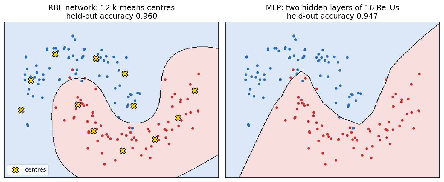
Twelve bumps and a least-squares output layer give 0.953 test accuracy on the moons split, on par with the RBF-SVM that keeps dozens of support vectors. Figure 5 (left) shows the same network with a logistic output layer.
Decision trees
In plain words. A decision tree plays twenty questions with the data. Each question looks at one feature and asks “is it at most this threshold?” Each answer sends the point left or right, until it reaches a leaf that holds a label. The tree is grown greedily: at every step, pick the question that makes the two resulting groups as “pure” as possible.
Impurity measures
Let a node contain training points with class proportions (fraction of the node’s points in each class ). An impurity function is zero when one class has all the points and largest when the classes are evenly mixed. The three standard choices are
The Gini index is the probability that two points drawn at random (with replacement) from the node have different labels. Entropy is the information-theoretic uncertainty of the label, in bits. Misclassification error is the error rate if the node predicted its majority class. Figure 4 (left) plots the three for two classes.
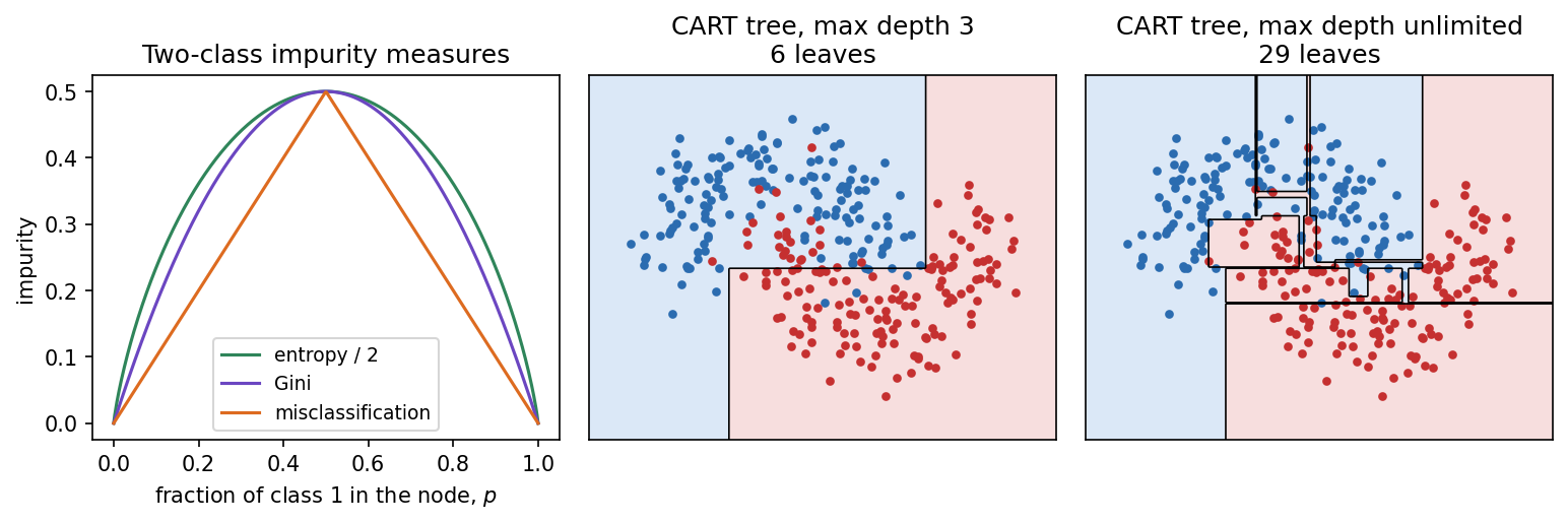
Gini and entropy are strictly concave, so splitting a node never increases their weighted average. Misclassification error is piecewise linear and often fails to reward a split that makes the children purer without changing either child’s majority label. That is why trees are grown with Gini or entropy and evaluated with error rate.
Growing a tree: the CART algorithm
The CART procedure of Breiman, Friedman, Olshen and Stone [12] grows a binary tree top-down. At a node with point set , it considers every feature and every threshold between consecutive observed values, splitting into and . It chooses the split with the largest impurity decrease
where is the chosen impurity and counts the points in a set. It then recurses on both children until a stopping rule fires (pure node, minimum node size, maximum depth). Quinlan’s ID3 [13] is a close relative that uses entropy, calls the information gain, and makes multiway splits on categorical features.
The code finds the best root split by brute force and checks it against scikit-learn, whose DecisionTreeClassifier implements an optimized version of CART.
Code · Python · 26 lines
import numpy as np
from sklearn.datasets import make_moons
from sklearn.tree import DecisionTreeClassifier

def gini(labels):
    p = np.bincount(labels, minlength=2) / len(labels)
    return 1.0 - (p ** 2).sum()

def best_split(X, y):
    best = (np.inf, None, None)
    for j in range(X.shape[1]):
        values = np.unique(X[:, j])
        for thr in (values[:-1] + values[1:]) / 2:
            left = X[:, j] <= thr
            n_l, n_r = left.sum(), (~left).sum()
            score = (n_l * gini(y[left]) + n_r * gini(y[~left])) / len(y)
            if score < best[0]:
                best = (score, j, thr)
    return best

X, y = make_moons(n_samples=300, noise=0.25, random_state=1)
score, j, thr = best_split(X, y)
root = DecisionTreeClassifier(max_depth=1).fit(X, y).tree_
print(f"ours: feature {j}, threshold {thr:.4f}, weighted Gini {score:.4f}")
print(f"sklearn: feature {root.feature[0]}, threshold {root.threshold[0]:.4f}")
assert j == root.feature[0] and np.isclose(thr, root.threshold[0])
Both choose feature 1 with threshold 0.0547, reducing the impurity from 0.5 at the root to a weighted 0.287.
Pruning and the character of trees
A tree grown until every leaf is pure memorizes the training set (Figure 4, right). CART’s answer is cost-complexity pruning [12]: grow a large tree , then for each subtree obtained by collapsing internal nodes, measure
where is the training misclassification rate, is the number of leaves and is a complexity price. Increasing traces a nested sequence of smaller and smaller trees; choose by cross-validation (ccp_alpha in scikit-learn).
Trees have a distinctive profile. They need no feature scaling, handle mixed numeric and categorical inputs, ignore irrelevant features if they never help a split, and produce rules a person can read. Their boundaries are axis-aligned staircases, so a diagonal boundary costs many splits. And they are unstable: a small change in the data can change the root split and hence the whole tree. Averaging many randomized trees (bagging, random forests) or adding them sequentially (boosting) fixes the instability, and that is the topic of PR 09.
Multilayer perceptrons as nonlinear classifiers
In plain words. A multilayer perceptron (MLP) is an RBF network whose bumps are replaced by learned “ramps,” and whose ramps are themselves learned from the labels. Each hidden unit draws one line; the next layer combines the lines into curved regions.
A one-hidden-layer MLP for classes computes
where map the inputs to hidden units, is an elementwise nonlinearity (ReLU , logistic or ), and map hidden units to class scores. All weights are trained jointly by minimizing cross-entropy with gradient descent, the gradients being computed by backpropagation [14]. Unlike every method above, both the features () and the classifier are learned from the labels. The universal approximation theorems of Cybenko [15] and Hornik [16] guarantee that one hidden layer with enough units can approximate any continuous function on a compact set; they say nothing about how many units are needed or whether gradient descent will find them. The full story, from neurons and activations to backpropagation and training tricks, is in ML 02; the image-classification version is in IP 13.
Geometrically, with ReLU units each hidden unit splits the input space with a hyperplane, and the network output is piecewise linear on the resulting cells, which is why the MLP boundary in Figure 5 is made of straight segments.
Code · Python · 16 lines
from sklearn.datasets import make_moons
from sklearn.model_selection import train_test_split
from sklearn.neural_network import MLPClassifier
from sklearn.pipeline import make_pipeline
from sklearn.preprocessing import StandardScaler

X, y = make_moons(n_samples=500, noise=0.18, random_state=2)
Xtr, Xte, ytr, yte = train_test_split(
    X, y, test_size=0.3, stratify=y, random_state=2)
for hidden in [(2,), (16,), (16, 16)]:
    mlp = make_pipeline(
        StandardScaler(),
        MLPClassifier(hidden_layer_sizes=hidden, alpha=1e-3,
                      max_iter=3000, random_state=0))
    mlp.fit(Xtr, ytr)
    print(hidden, "test accuracy:", round(mlp.score(Xte, yte), 4))
With two hidden units the network can only bend the boundary once and reaches 0.833. Sixteen units reach 0.947, and a second layer of 16 does not help on this easy two-dimensional problem. Depth pays off on high-dimensional inputs such as images, where it lets the network build features hierarchically (ML 03).
Choosing among nonlinear classifiers
| Method | Boundary shape | Training cost | Prediction cost | Key hyperparameters | Typical strengths |
|---|---|---|---|---|---|
| -NN | Any; follows data | None (store data) | per query | , metric, scaling | Simple baseline; good with good embeddings |
| Kernel SVM | Smooth (RBF) | Roughly – | , kernel, | Small/medium data, strong theory | |
| Gaussian process | Smooth, with uncertainty | exact | mean, variance | Kernel; set by marginal likelihood | Calibrated uncertainty (regression) |
| RBF network | Smooth, local | Clustering + linear solve | , | Cheap prediction | |
| Decision tree | Axis-aligned boxes | per level | Depth, leaf size, | Interpretable; mixed feature types | |
| MLP | Piecewise linear (ReLU) | Iterative SGD | Width, depth, decay, learning rate | Scales to large data; learns features |
Here is the number of support vectors and the number of RBF centers. The complexity entries are orders of magnitude, not exact counts. No row wins everywhere. Compare candidates under one validation protocol, and remember the lesson of the grid-search example: differences of a fraction of a percent on one split are rarely real.
Modern view
Kernel methods dominated pattern recognition from the late 1990s until deep networks took over large-scale perception around 2012. They did not disappear; they changed roles. Six strands summarize the current picture.
Surveys of the classical field. Hofmann, Schölkopf and Smola’s review in the Annals of Statistics [7] is the standard map of kernel methods: positive definite kernels and their RKHS, the representer theorem, kernel construction for structured data such as strings and graphs, and the statistical learning theory behind large margins. Cervantes et al. [19] survey SVM classification from the application side: variants developed where the basic SVM struggles (very large data sets, many classes, imbalanced classes), combinations with evolutionary parameter search, a long catalogue of applications, and the method’s limitations. For trees, Costa and Pedreira [20] review recent decision-tree research around the three goals of any predictive learner: fitting the training data, generalizing beyond it, and staying interpretable.
Scaling kernels. The memory of a Gram matrix was the main barrier. Rahimi and Recht’s random features [17] approximate a shift-invariant kernel such as the RBF by an explicit random map with , so that a linear model on random features stands in for the kernel machine. Liu et al.’s survey [18] organizes a decade of follow-ups: sampling schemes for the random features, theory on how many features are needed for a given accuracy, and connections to deep networks. Combining such approximations with GPU linear algebra, the FALKON line of work trains kernel ridge regression on billions of points [23], and GPyTorch [24] makes exact and approximate Gaussian process inference practical on GPUs with iterative matrix–matrix solvers.
Kernels as a lens on deep learning. Jacot, Gabriel and Hongler showed that, in an infinite-width limit with suitable scaling, training a neural network by gradient descent is equivalent to kernel regression with a fixed neural tangent kernel [21]. Belkin, Ma and Mandal argued that phenomena puzzling in deep learning, such as fitting the training data exactly yet still generalizing, already appear in kernel machines, so understanding kernels is a prerequisite for understanding deep networks [22]. Real networks of finite width do learn their features, which a fixed kernel cannot, so this analogy is a theoretical tool, not a replacement.
Trees still rule tabular data. For data in tables (rows of heterogeneous measurements rather than pixels or words), Grinsztajn, Oyallon and Varoquaux benchmarked tree ensembles against deep architectures on 45 medium-sized datasets and found the tree-based models still ahead, attributing the gap to neural networks’ sensitivity to uninformative features, their rotation invariance, and their bias toward smooth functions [25]. The newest challenger is a tabular foundation model: TabPFN, a transformer trained across millions of synthetic datasets, predicts on a new small dataset in a single forward pass. Its authors report that it outperforms previous methods, including tuned gradient-boosted tree ensembles, on datasets with up to 10,000 samples, with far less training time [26].
Neighbors on learned features. The nearest-neighbor rule has had a revival as a classifier on top of large pretrained embeddings. Once features are good, a -NN or cosine-similarity classifier is often the simplest strong baseline, and it can add new classes without retraining. IP 13 and ML 06 discuss this pattern.
Open problems. Exact kernel methods and GPs still scale poorly in ; approximation quality versus speed remains an active trade-off [18]. Choosing kernels for structured data is still largely manual. Single trees remain unstable, and globally optimal trees are expensive to compute [20]. And for tabular data, whether foundation-style models will displace tuned tree ensembles beyond small datasets is an open question as of 2026.
Key takeaways
- Nonlinear boundaries come from three ideas: comparing with stored examples (-NN), lifting to a feature space where a linear rule works (kernels, RBF networks, MLPs), or partitioning the space (trees).
- -NN’s behavior is set by the metric and scaling as much as by ; for unit vectors, Euclidean and cosine neighbors coincide.
- A kernel is valid exactly when every Gram matrix is symmetric positive semidefinite (Mercer’s condition). The kernel trick replaces inner products by kernel values in any algorithm written in inner products.
- The soft-margin SVM minimizes plus times hinge loss. Its dual depends on the data only through the kernel, and only support vectors () affect predictions. Tune and jointly, on standardized features, by cross-validation.
- GPs give kernel predictions with uncertainty; the RVM (Tipping) gives sparse probabilistic kernel models. SVM scores are not probabilities.
- RBF networks use a few explicit Gaussian bumps; trees grow greedily by impurity decrease (Gini or entropy) and need pruning; MLPs learn their own features and are covered in depth in ML 02.
- No family wins everywhere: kernels for small/medium smooth problems, trees and their ensembles for tabular data, deep networks for raw perceptual data, neighbors on top of good embeddings.
Exercises
- Distance and cosine. Derive for unit vectors, and show that the 1-NN under Euclidean distance equals the 1-NN under cosine similarity. Does this still hold if the vectors are not normalized?
Hint
Expand . With unit norms, distance is a decreasing function of , so the minimizer of one is the maximizer of the other. Without normalization the norms enter: a long vector pointing in a slightly different direction can be closer in Euclidean distance than a short, perfectly aligned one.
- Building a kernel. Show that is a valid kernel in by writing down its feature map. Then use the closure rules to argue that the Gaussian kernel is valid.
Hint
. For the Gaussian, write . The middle factor is of a valid (scaled linear) kernel, and the outer factors have the form .
- The limits of . For a fixed finite data set, what does the RBF Gram matrix tend to as and as ? Relate each limit to the leftmost and rightmost columns of Figure 2.
Hint
As every entry tends to 1 (the all-ones matrix): all points look alike and the boundary becomes nearly linear or constant. As the off-diagonal entries tend to 0 and : each point is only similar to itself, so the SVM can memorize every training label, which is the “islands” regime.
- Support vectors and cost. An RBF-SVM trained on 100,000 images keeps 90% of them as support vectors. What does this imply about the data and about prediction time? Name two things you could try.
Hint
Many points sit inside the margin or are misclassified: the classes overlap heavily in this feature space, or is small or is badly chosen. Each prediction needs about 90,000 kernel evaluations. Try re-tuning and , better features, random features with a linear SVM, or a different model family.
- Impurity by hand. A node has 40 points of class A and 40 of class B. Split 1 gives children (30 A, 10 B) and (10 A, 30 B). Split 2 gives (40 A, 20 B) and (0 A, 20 B). Compute the misclassification-error decrease and the Gini decrease for both splits. Which split does each measure prefer?
Hint
Root Gini , root error . Split 1: both children have error and Gini ; weighted error , weighted Gini . Split 2: left child error , Gini ; right child pure. Weighted error , weighted Gini . Error cannot tell them apart (both 0.25); Gini prefers split 2, which creates a pure node.
- RBF network design. In the RBF-network code, vary and . Which combinations underfit and which overfit? Why does a small with a large behave badly?
Hint
With few centers and a large , the bumps are narrow and most points activate none of them strongly, so the design matrix is nearly zero away from the centers and the classifier falls back to the bias. Many centers with a large start to behave like a kernel machine with too little regularization.
References
-
S. Theodoridis and K. Koutroumbas, Pattern Recognition, 4th ed., Academic Press, 2009, Chapters 2 and 4. publisher page
-
C. M. Bishop, Pattern Recognition and Machine Learning, Springer, 2006, Sections 2.5.2, 5.1–5.3, 6.1–6.4, 7.1–7.2 and 14.4. official book page and PDF
-
T. Cover and P. Hart, “Nearest Neighbor Pattern Classification,” IEEE Transactions on Information Theory, vol. 13, no. 1, pp. 21–27, 1967. doi:10.1109/TIT.1967.1053964
-
J. Mercer, “Functions of Positive and Negative Type, and Their Connection with the Theory of Integral Equations,” Philosophical Transactions of the Royal Society of London, Series A, vol. 209, pp. 415–446, 1909. doi:10.1098/rsta.1909.0016
-
B. E. Boser, I. M. Guyon, and V. N. Vapnik, “A Training Algorithm for Optimal Margin Classifiers,” Proceedings of the Fifth Annual Workshop on Computational Learning Theory (COLT), pp. 144–152, 1992. doi:10.1145/130385.130401
-
C. Cortes and V. Vapnik, “Support-Vector Networks,” Machine Learning, vol. 20, pp. 273–297, 1995. doi:10.1007/BF00994018
-
T. Hofmann, B. Schölkopf, and A. J. Smola, “Kernel Methods in Machine Learning,” The Annals of Statistics, vol. 36, no. 3, 2008. doi:10.1214/009053607000000677
-
C. E. Rasmussen and C. K. I. Williams, Gaussian Processes for Machine Learning, MIT Press, 2006. book page
-
M. E. Tipping, “Sparse Bayesian Learning and the Relevance Vector Machine,” Journal of Machine Learning Research, vol. 1, pp. 211–244, 2001. JMLR
-
J. Moody and C. J. Darken, “Fast Learning in Networks of Locally-Tuned Processing Units,” Neural Computation, vol. 1, no. 2, pp. 281–294, 1989. doi:10.1162/neco.1989.1.2.281
-
J. Park and I. W. Sandberg, “Universal Approximation Using Radial-Basis-Function Networks,” Neural Computation, vol. 3, no. 2, pp. 246–257, 1991. doi:10.1162/neco.1991.3.2.246
-
L. Breiman, J. H. Friedman, R. A. Olshen, and C. J. Stone, Classification and Regression Trees, Chapman and Hall/CRC, 2017 edition. doi:10.1201/9781315139470
-
J. R. Quinlan, “Induction of Decision Trees,” Machine Learning, vol. 1, pp. 81–106, 1986. doi:10.1007/BF00116251
-
D. E. Rumelhart, G. E. Hinton, and R. J. Williams, “Learning Representations by Back-Propagating Errors,” Nature, vol. 323, pp. 533–536, 1986. doi:10.1038/323533a0
-
G. Cybenko, “Approximation by Superpositions of a Sigmoidal Function,” Mathematics of Control, Signals, and Systems, vol. 2, pp. 303–314, 1989. doi:10.1007/BF02551274
-
K. Hornik, “Approximation Capabilities of Multilayer Feedforward Networks,” Neural Networks, vol. 4, no. 2, pp. 251–257, 1991. doi:10.1016/0893-6080(91)90009-T
-
A. Rahimi and B. Recht, “Random Features for Large-Scale Kernel Machines,” Advances in Neural Information Processing Systems 20 (NIPS), 2007. paper
-
F. Liu, X. Huang, Y. Chen, and J. A. K. Suykens, “Random Features for Kernel Approximation: A Survey on Algorithms, Theory, and Beyond,” IEEE Transactions on Pattern Analysis and Machine Intelligence, vol. 44, no. 10, pp. 7128–7148, 2022. doi:10.1109/TPAMI.2021.3097011
-
J. Cervantes, F. Garcia-Lamont, L. Rodríguez-Mazahua, and A. Lopez, “A Comprehensive Survey on Support Vector Machine Classification: Applications, Challenges and Trends,” Neurocomputing, vol. 408, pp. 189–215, 2020. doi:10.1016/j.neucom.2019.10.118
-
V. G. Costa and C. E. Pedreira, “Recent Advances in Decision Trees: An Updated Survey,” Artificial Intelligence Review, vol. 56, pp. 4765–4800, 2023. doi:10.1007/s10462-022-10275-5
-
A. Jacot, F. Gabriel, and C. Hongler, “Neural Tangent Kernel: Convergence and Generalization in Neural Networks,” NeurIPS, 2018. arXiv:1806.07572
-
M. Belkin, S. Ma, and S. Mandal, “To Understand Deep Learning We Need to Understand Kernel Learning,” arXiv:1802.01396, 2018. arXiv
-
G. Meanti, L. Carratino, L. Rosasco, and A. Rudi, “Kernel Methods Through the Roof: Handling Billions of Points Efficiently,” Advances in Neural Information Processing Systems 33 (NeurIPS), 2020. paper
-
J. R. Gardner, G. Pleiss, D. Bindel, K. Q. Weinberger, and A. G. Wilson, “GPyTorch: Blackbox Matrix-Matrix Gaussian Process Inference with GPU Acceleration,” NeurIPS, 2018. arXiv:1809.11165
-
L. Grinsztajn, E. Oyallon, and G. Varoquaux, “Why Do Tree-Based Models Still Outperform Deep Learning on Typical Tabular Data?,” Advances in Neural Information Processing Systems 35 (NeurIPS), Datasets and Benchmarks Track, 2022. paper
-
N. Hollmann, S. Müller, L. Purucker, A. Krishnakumar, et al., “Accurate Predictions on Small Data with a Tabular Foundation Model,” Nature, vol. 637, pp. 319–326, 2025. doi:10.1038/s41586-024-08328-6
-
scikit-learn developers, “Support Vector Machines,” user guide, accessed 2026-11-05. documentation
Check your understanding
This tutorial has 6 exercises. Can you solve them without opening the hints?
Go to the exercises ↑Next PR 05 · Feature Selection, Transforms and Dimensionality · 25 min