PR 07 · Clustering, Mixtures and EM
Needs: PR 06 · Template Matching and Structured Recognition
Navigate: this page and this track: Navigate: this page and this track
On this page
- What you’ll learn1 min
- The big picture2 min
- Similarity, scaling and what “a cluster” means1 min
- K-means and Lloyd’s algorithm4 min
- Hierarchical clustering2 min
- Density-based clustering: DBSCAN2 min
- Spectral clustering in one page1 min
- Code: one geometry, different assumptions1 min
- Gaussian mixtures and the EM algorithm4 min
- Choosing the number of clusters2 min
- Cluster validity: is the clustering any good?2 min
- Modern view3 min
- Key takeaways1 min
- Exercises2 min
- References
Pattern Recognition
Explore this chapter 1 interactive experiment
Step through Gaussian-mixture EM and observe responsibilities, likelihood and the symmetric-initialization trap.
What you’ll learn
- What a clustering algorithm actually optimizes, and why the choice of features, scaling and distance decides the answer before any algorithm runs.
- How Lloyd’s k-means works, why it always converges but only to a local optimum, and how k-means++ seeding gives a provable guarantee.
- How hierarchical clustering (single, complete, average and Ward linkage), DBSCAN and spectral clustering encode different definitions of “a group”.
- How to derive the E and M steps of expectation–maximization (EM) for a Gaussian mixture from scratch, why EM never decreases the likelihood, and where it can fail.
- How to choose the number of clusters with BIC and AIC, and how to read internal indices (silhouette, Davies–Bouldin, Calinski–Harabasz), external indices (ARI, NMI) and stability.
The big picture
So far in this track every training example came with a label. Clustering removes the labels and asks: are there natural groups in the data? The answer is never fully determined by the data alone. The same collection of images can be grouped by object, by color, by background or by the camera that took them. Each grouping is “correct” under its own notion of similarity. A clustering algorithm is therefore a precise statement of which notion of similarity we mean, plus a search procedure for the best grouping under that notion.
Why it matters in recognition: clustering builds visual vocabularies (local image descriptors quantized with k-means into “visual words”), initializes and compresses models (vector quantization, color palettes), discovers sub-classes inside a labeled class, finds outliers, segments images (pixel clustering, see IP 10), and, in modern self-supervised learning, produces pseudo-labels for training deep networks. Gaussian mixtures are also the standard example of a latent-variable model, and EM is the template for many inference algorithms we will meet in PR 08.
This chapter follows the clustering part of Theodoridis and Koutroumbas (Chapters 11–16) [1] and Bishop’s Chapter 9 on mixtures and EM [2]. It organizes the main algorithm families, derives the two most important ones in full, and ends with how to decide whether a clustering is any good.
Similarity, scaling and what “a cluster” means
Plain version. Before choosing an algorithm, decide what “close” means. Change the features or their units and the clusters change.
Precise version. Most methods start from a dissimilarity between feature vectors . Common choices are
where is the Euclidean distance, is the Mahalanobis distance with a positive-definite matrix (often a covariance estimate), and is the cosine dissimilarity, which ignores vector length and is popular for deep-network embeddings.
Three practical consequences follow.
- Scaling is a modeling decision. If one coordinate is measured in millimeters and another in kilometers, Euclidean distance is dominated by the first. Standardizing every feature to unit variance removes that, but it also removes any genuinely meaningful difference in spread. For classification we can let validation decide; for clustering there are no labels, so the choice must come from domain knowledge.
- Hard versus soft assignments. A hard partition assigns each point to exactly one cluster . A soft assignment stores degrees of membership with . In a Gaussian mixture these are posterior probabilities; in fuzzy clustering [1] they are memberships defined by an objective and should not be read as probabilities.
- Clusters are not classes. Labels are attached to clusters afterwards and arbitrarily. Cluster “3” in one run may be cluster “1” in the next, so any comparison with class labels must be invariant to permutations, which is exactly what ARI and NMI (below) are.
Theodoridis and Koutroumbas classify algorithms into sequential, hierarchical, objective-function-based (k-means, mixtures, fuzzy), and graph/density-based families [1]. We follow roughly that order.
K-means and Lloyd’s algorithm
Plain version. Choose centers. Repeat two steps: give every point to its nearest center, then move every center to the average of its points. Stop when nothing changes.
The objective
With one-hot indicators ( if point is in cluster , and ) and centers , k-means minimizes the within-cluster sum of squares
Here is the number of points and their dimension. is also called inertia or distortion.
Two alternating steps
Lloyd’s algorithm [3] (developed for quantizing signals in pulse-code modulation) minimizes by block coordinate descent:
- Assignment step. Fix . Each term involves a single , so set for .
- Update step. Fix . is a convex quadratic in each ; setting the gradient to zero,
the mean of the points currently in cluster . The name “k-means” was coined by MacQueen [4], whose version updates a center immediately after each point arrives, , where is the running count of points in cluster .
Why it converges, and why only locally
Each step can only lower or leave it unchanged: the assignment step picks the best for the current , and the update step picks the best for the current . There are finitely many partitions of points into groups, and (with a consistent tie-breaking rule) the algorithm never revisits a partition with a higher , so it stops after finitely many iterations. The fixed point is a local minimum: a partition where no single step helps. Different initial centers can lead to very different fixed points.
Two implementation details matter. An empty cluster (no point assigned) has no mean; common rules keep the old center or re-seed it at the point with the largest current error. And every iteration costs distance computations, which motivates the mini-batch variant below.
What k-means assumes
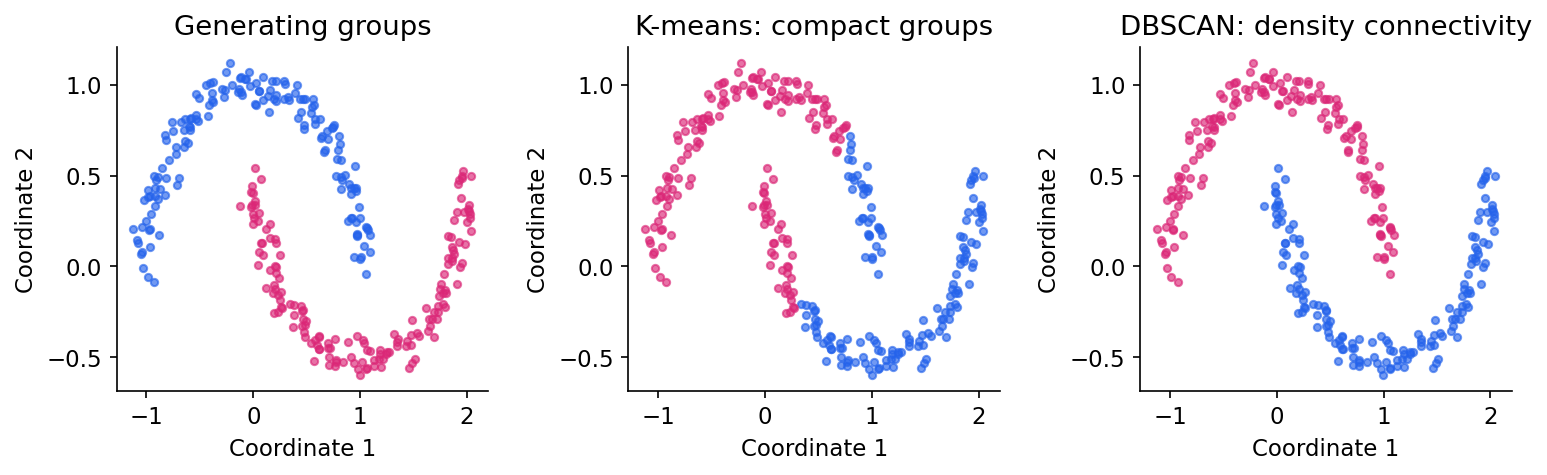
Because the objective is a sum of squared Euclidean distances to a center, the boundary between two clusters is the perpendicular bisector of their centers: k-means partitions space into Voronoi cells. It works well for compact, roughly spherical groups of similar size. It splits elongated groups, merges small groups that are close to large ones, and cannot follow curved shapes (Figure 1, middle).
k-means++ seeding
Plain version. Start with one random center, then pick each new center far from the ones you already have, but randomly, so outliers do not always win.
Arthur and Vassilvitskii [5] proposed D² seeding:
- Pick the first center uniformly at random from the data.
- For every point compute , the distance to the nearest center chosen so far.
- Pick the next center as with probability .
- Repeat steps 2–3 until centers are chosen, then run Lloyd’s algorithm.
Their main theorem states that the seeding alone already achieves, in expectation,
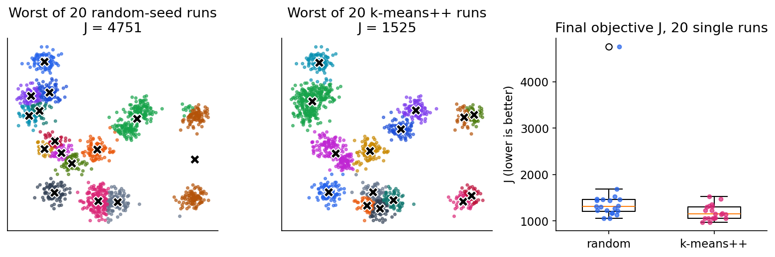
where is the optimal k-means objective. Lloyd iterations can only lower further. Uniform random seeding has no such guarantee. The bound is a worst-case statement; in practice the benefit shows up mostly as fewer catastrophic runs. Libraries combine k-means++ with several restarts (n_init in scikit-learn) and keep the run with the lowest .
Code: k-means++ and Lloyd from scratch
Code · Python · 46 lines
import numpy as np
from sklearn.datasets import make_blobs
from sklearn.cluster import KMeans

def kmeans_pp_init(X, k, rng):
    """D^2 seeding: each new center is drawn with probability proportional
    to the squared distance to the nearest center chosen so far."""
    centers = [X[rng.integers(len(X))]]
    for _ in range(k - 1):
        d2 = np.min(((X[:, None, :] - np.array(centers)[None]) ** 2).sum(-1), axis=1)
        centers.append(X[rng.choice(len(X), p=d2 / d2.sum())])
    return np.array(centers)

def lloyd(X, centers, max_iter=100):
    history = []
    for _ in range(max_iter):
        d2 = ((X[:, None, :] - centers[None]) ** 2).sum(-1)   # N x K
        z = d2.argmin(axis=1)                                 # assignment step
        history.append(d2[np.arange(len(X)), z].sum())        # objective J
        new = np.array([X[z == k].mean(axis=0) if np.any(z == k) else centers[k]
                        for k in range(len(centers))])        # update step
        if np.allclose(new, centers):
            break
        centers = new
    return centers, z, history

X, _ = make_blobs(n_samples=600, centers=4, cluster_std=1.8, random_state=7)
rng = np.random.default_rng(0)
best = None
for restart in range(10):                      # several seeds, keep the best J
    c, z, hist = lloyd(X, kmeans_pp_init(X, 4, rng))
    if best is None or hist[-1] < best[2][-1]:
        best = (c, z, hist)
c, z, hist = best
print("J per iteration:", np.round(hist, 1))
assert all(a >= b - 1e-9 for a, b in zip(hist, hist[1:]))   # monotone
ref = KMeans(n_clusters=4, n_init=10, random_state=0).fit(X)
print("from scratch J:", round(hist[-1], 2), " sklearn inertia:", round(ref.inertia_, 2))

# single runs (no restarts): uniform random seeding vs D^2 seeding, 15 clusters
X2, _ = make_blobs(n_samples=1500, centers=15, cluster_std=0.6, random_state=2)
for name, init in [("random", lambda r: X2[r.choice(len(X2), 15, replace=False)]),
                   ("k-means++", lambda r: kmeans_pp_init(X2, 15, r))]:
    finals = [lloyd(X2, init(np.random.default_rng(s)))[2][-1] for s in range(20)]
    print(f"{name:9s} final J over 20 runs: median {np.median(finals):7.1f}, "
          f"worst {np.max(finals):7.1f}")
Output (NumPy 2.0, scikit-learn 1.6):
Code · 4 lines
J per iteration: [5865.6 3633.4 3625. ]
from scratch J: 3625.0  sklearn inertia: 3625.0
random    final J over 20 runs: median  1305.1, worst  4750.8
k-means++ final J over 20 runs: median  1147.5, worst  1525.2
The from-scratch version reaches the same objective as scikit-learn, and decreases monotonically. On the 15-cluster problem, uniform seeding sometimes puts two seeds in one blob and none in another; Lloyd’s algorithm cannot repair that, and the worst run is about three times worse. Figure 2 shows the two worst runs.
Mini-batch k-means
For millions of points, Sculley’s mini-batch k-means [6] updates the centers using small random batches: each center moves toward the batch points assigned to it with a per-center learning rate that decays as . It trades a slightly higher final objective for a large speed-up, and is available as MiniBatchKMeans in scikit-learn. It is the usual choice for building large visual vocabularies.
Hierarchical clustering
Plain version. Start with every point as its own group. Repeatedly merge the two closest groups. The record of merges is a tree; cut it at some height to get clusters.
Agglomerative algorithm and linkages
Agglomerative clustering needs a definition of the distance between two groups and . The four classical linkages are
where is the number of points in and are the group means. Ward’s criterion [7] is the increase of the within-cluster sum of squares caused by merging and , so Ward agglomeration is a greedy, bottom-up way of keeping small, the same objective as k-means.
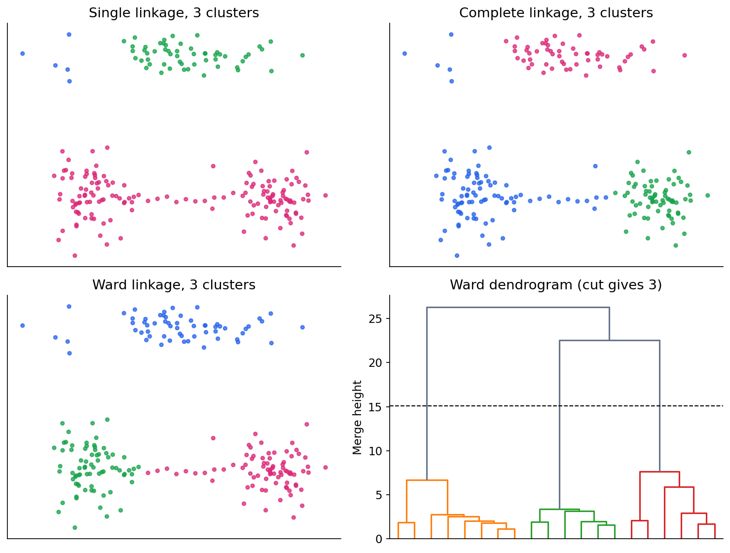
Each linkage has a personality (Figure 3):
- Single linkage merges whenever any two points are close. It follows arbitrary shapes, but a thin “bridge” of points can chain two groups together. It is equivalent to cutting the longest edges of a minimum spanning tree, one of the graph-based methods in [1].
- Complete linkage requires all pairs to be close. It produces compact groups of similar diameter and is sensitive to outliers.
- Average linkage sits between the two.
- Ward produces compact, similarly sized, roughly spherical groups, much like k-means.
The dendrogram
The merge history is a binary tree called a dendrogram; the height of each junction is the linkage value at which the merge happened. Cutting the tree at height yields the partition at that level, and a large gap between consecutive merge heights suggests a natural number of clusters. The cut height is still a choice.
Two practical limitations: merges are never undone, so an early mistake propagates; and the standard algorithm stores all pairwise distances, memory, which limits it to tens of thousands of points. Divisive (top-down) hierarchical methods exist but are less common.
Density-based clustering: DBSCAN
Plain version. A cluster is a crowded region. Points in crowded places grow the cluster; points in empty places are labeled noise.
DBSCAN (Density-Based Spatial Clustering of Applications with Noise) [8] has two parameters, a radius and a count . Let be the -neighborhood of (including itself). Then
- is a core point if ;
- is a border point if it is not core but lies in the -neighborhood of some core point;
- every other point is noise.
A point is density-reachable from a core point if there is a chain of core points, each within of the next, ending in its neighborhood. A cluster is a maximal set of mutually density-connected points. DBSCAN finds clusters of any shape, does not need , and explicitly refuses to assign isolated points.
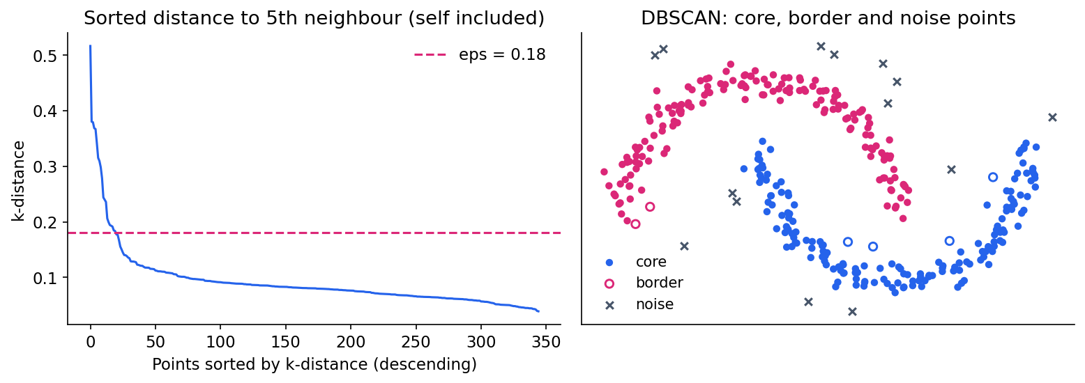
Choosing . The original paper suggests the sorted k-distance graph: for each point compute the distance to its -th nearest neighbor with , sort these values, and pick near the “knee” where the curve rises sharply (Figure 4, left). In the descending plot of Figure 4 the large values to the left of the knee are the candidates for noise. scikit-learn’s min_samples counts the point itself, which matches the definition above.
Limitations. A single means a single density level. If one cluster is dense and another sparse, no separates both. In high dimensions, distances concentrate and the neighborhood counts lose contrast. HDBSCAN [9] addresses the first issue by building a hierarchy over all density levels and extracting the most stable clusters, replacing with a minimum cluster size; it is available as HDBSCAN in scikit-learn.
Spectral clustering in one page
Plain version. Build a graph that connects nearby points, then find the cuts that sever the fewest strong connections.
Given an affinity matrix (, large for similar points, for example a -nearest-neighbor graph or ) and the diagonal degree matrix , one normalized graph Laplacian is
If the graph has connected components, has eigenvalue with multiplicity , and its eigenvectors indicate the components. For a nearly disconnected graph, the eigenvectors with the smallest eigenvalues still nearly indicate the groups. Spectral clustering stacks these eigenvectors as columns, normalizes the rows, and runs k-means on the rows [10]. The result can follow curved shapes that defeat k-means in the original space, because the eigenvectors measure connectivity, not distance to a center.
The graph is part of the model. The neighborhood size or bandwidth must be chosen; a graph that is accidentally disconnected (an isolated vertex, say) produces a trivial eigenvector that dominates the result. Von Luxburg’s tutorial [10] explains the graph-cut interpretation (ratio cut and normalized cut) and gives practical advice on choosing the graph.
Code: one geometry, different assumptions
The two-moons data set below is generated with labels, but the labels are used only to score each result afterwards with the adjusted Rand index (ARI, 1 = perfect agreement up to relabeling, about 0 = chance).
Code · Python · 30 lines
import numpy as np
from sklearn.datasets import make_moons
from sklearn.neighbors import NearestNeighbors
from sklearn.cluster import (KMeans, AgglomerativeClustering, DBSCAN,
                             HDBSCAN, SpectralClustering)
from sklearn.mixture import GaussianMixture
from sklearn.metrics import adjusted_rand_score

X, truth = make_moons(n_samples=320, noise=0.06, random_state=5)

# k-distance curve for choosing DBSCAN's eps (k = min_samples)
dist, _ = NearestNeighbors(n_neighbors=5).fit(X).kneighbors(X)
kdist = np.sort(dist[:, -1])                    # 5th neighbour, counting the point itself
print("k-distance quantiles 50/90/99%:", np.round(np.quantile(kdist, [0.5, 0.9, 0.99]), 3))

models = {
    "k-means": KMeans(n_clusters=2, n_init=10, random_state=5),
    "single linkage": AgglomerativeClustering(n_clusters=2, linkage="single"),
    "Ward linkage": AgglomerativeClustering(n_clusters=2, linkage="ward"),
    "Gaussian mixture": GaussianMixture(n_components=2, n_init=3, random_state=5),
    "DBSCAN": DBSCAN(eps=0.18, min_samples=5),
    "HDBSCAN": HDBSCAN(min_cluster_size=15),
    "spectral": SpectralClustering(n_clusters=2, affinity="nearest_neighbors",
                                   n_neighbors=20, assign_labels="kmeans",
                                   random_state=5),
}
for name, model in models.items():
    labels = model.fit_predict(X)
    print(f"{name:17s} ARI = {adjusted_rand_score(truth, labels):.3f}"
          f"   noise points = {int((labels == -1).sum())}")
Output
k-distance quantiles 50/90/99%: [0.079 0.11  0.144]
k-means           ARI = 0.260   noise points = 0
single linkage    ARI = 1.000   noise points = 0
Ward linkage      ARI = 0.242   noise points = 0
Gaussian mixture  ARI = 0.488   noise points = 0
DBSCAN            ARI = 1.000   noise points = 0
HDBSCAN           ARI = 0.988   noise points = 2
spectral          ARI = 1.000   noise points = 0
Figure 1 shows two of these results. Methods built on centers or ellipses (k-means, Ward, a two-component Gaussian mixture) cut each moon in half; connectivity-based methods (single linkage, DBSCAN, HDBSCAN, spectral) recover the moons. The chosen lies above the 99th percentile of the k-distance, so no moon point is called noise. A -nearest-neighbor graph with too few neighbors can be disconnected, and scikit-learn then warns that the spectral embedding may be unreliable; neighbors avoids that here. None of this makes connectivity methods “better”: on overlapping Gaussian blobs single linkage chains everything together and k-means wins. Comparisons must vary geometry, density, noise and dimension.
Gaussian mixtures and the EM algorithm
Plain version. Pretend every point was produced by first rolling a -sided die to pick a cloud, then sampling from that Gaussian cloud. We never see the die. EM guesses, for every point, how likely each cloud produced it (E step), then refits each cloud using those guesses as weights (M step), and repeats.
The model
A Gaussian mixture model (GMM) with components has density
where is the mixing weight (prior probability of component ), its mean, its covariance, collects all parameters, and
Introduce a latent one-hot variable with and . Summing out gives back the mixture density. Given data , the log-likelihood is
The logarithm of a sum couples all the parameters, so setting its gradient to zero has no closed-form solution. EM is the standard way around this [11], [2].
Step 1: the complete-data log-likelihood
If we knew the assignments , the log-likelihood of would be
The logarithm now acts on a single Gaussian, and the problem splits into separate weighted Gaussian fits: easy.
Step 2 (E step): the expected complete-data log-likelihood
We do not know , but with current parameters we know its posterior. By Bayes’ rule,
evaluated at . The number is the responsibility of component for point ; each row sums to one. Because the complete-data log-likelihood is linear in , its expectation under this posterior simply replaces by :
Step 3 (M step): maximize in closed form
Define the effective count .
Mixing weights. Only depends on , under the constraint . With a Lagrange multiplier ,
Summing over gives , so . (The constraint is satisfied automatically.)
Means. The gradient with respect to is . Setting it to zero and multiplying by ,
Covariances. Write , so and the quadratic term is . Using and for symmetric ,
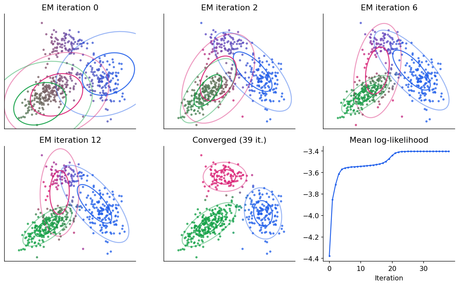
These are the familiar maximum-likelihood formulas for one Gaussian (see PR 02), with every point weighted by its responsibility. EM alternates the E step and the M step until the log-likelihood stops improving (Figure 5).
Why EM never decreases the likelihood
For any distribution over the latent assignments,
So is a lower bound on the log-likelihood, the evidence lower bound (ELBO). The E step sets , which makes the KL term zero and the bound tight at . The M step maximizes over ; since , this is the same as maximizing . The new likelihood is at least the new bound, which is at least the old bound, which equals the old likelihood. Hence [11], [2]. When the exact posterior is intractable, we restrict to a tractable family and get variational inference, the subject of PR 08.
Monotone does not mean globally optimal or safely convergent: under suitable regularity conditions EM can approach a stationary point, while an unconstrained Gaussian mixture can instead head toward the singularity described next. Practical implementations initialize from k-means and run several restarts.
Singularities and how to avoid them
The likelihood of an unconstrained GMM is unbounded. Put one component’s mean exactly on a data point, , with . That term contributes to , which goes to infinity as , while the other components keep the remaining points’ likelihood finite. The unrestricted maximum likelihood estimate therefore need not exist, and EM itself does not prevent collapse. Use a positive covariance floor (reg_covar in scikit-learn [26]), explicit variance constraints, or an appropriate prior. Diagonal or spherical covariance alone is not a cure: the collapsing covariance already has both forms. A simpler covariance reduces parameter count; it still needs protection against zero variance. Restarting a component is an operational response, not a proof that the unconstrained objective is bounded.
Identifiability and label switching
Permuting the component labels leaves the density unchanged, so there are equivalent maxima. “Component 2” has no inherent meaning, and comparing component indices with class labels requires a matching rule.
K-means as the limit of EM
Fix and for all . The responsibilities become
As , the term with the smallest distance dominates, so for the nearest center and otherwise: the E step becomes the k-means assignment step and the M step for becomes the k-means update [2]. A general GMM therefore extends k-means with soft assignments, unequal sizes () and elliptical shapes ().
Code: EM from scratch, checked against scikit-learn
Code · Python · 45 lines
import numpy as np
from scipy.special import logsumexp
from scipy.stats import multivariate_normal
from sklearn.mixture import GaussianMixture

rng = np.random.default_rng(3)
true_means = np.array([[0.0, 0.0], [4.0, 1.0], [1.0, 4.0]])
true_covs = [np.array([[1.0, 0.6], [0.6, 0.8]]),
             np.array([[0.5, -0.2], [-0.2, 1.2]]),
             np.array([[0.7, 0.0], [0.0, 0.3]])]
counts = [250, 150, 100]
X = np.vstack([rng.multivariate_normal(m, S, n)
               for m, S, n in zip(true_means, true_covs, counts)])
N, D = X.shape
K, reg = 3, 1e-6                               # reg: small covariance floor

# initialise with K random points, shared data covariance, equal weights
mu = X[rng.choice(N, K, replace=False)]
Sigma = np.array([np.cov(X.T) for _ in range(K)])
pi = np.full(K, 1.0 / K)
loglik = []
for it in range(200):
    # E step: log of pi_k N(x_n | mu_k, Sigma_k), normalised with log-sum-exp
    log_joint = np.column_stack([np.log(pi[k]) +
                                 multivariate_normal(mu[k], Sigma[k]).logpdf(X)
                                 for k in range(K)])
    log_norm = logsumexp(log_joint, axis=1)
    R = np.exp(log_joint - log_norm[:, None])     # responsibilities r_nk
    loglik.append(log_norm.sum())
    # M step: closed-form weighted updates
    Nk = R.sum(axis=0)
    pi = Nk / N
    mu = (R.T @ X) / Nk[:, None]
    for k in range(K):
        diff = X - mu[k]
        Sigma[k] = (R[:, k, None] * diff).T @ diff / Nk[k] + reg * np.eye(D)
    if it > 0 and loglik[-1] - loglik[-2] < 1e-8:
        break

assert np.all(np.diff(loglik) > -1e-6)           # EM never decreases log-likelihood
print("iterations:", len(loglik), " final mean log-lik:", round(loglik[-1] / N, 4))
print("weights:", np.round(np.sort(pi), 3))
gm = GaussianMixture(3, covariance_type="full", n_init=5, random_state=0).fit(X)
print("sklearn mean log-lik:", round(gm.score(X), 4))
print("sklearn weights:", np.round(np.sort(gm.weights_), 3))
Output
iterations: 40  final mean log-lik: -3.4032
weights: [0.202 0.299 0.499]
sklearn mean log-lik: -3.4033
sklearn weights: [0.203 0.3   0.497]
The E step works in log space: densities in high dimension underflow, and logsumexp computes stably. The recovered weights match the generating proportions and scikit-learn’s solution; the tiny difference comes from scikit-learn’s own stopping tolerance.
Choosing the number of clusters
Plain version. More clusters always fit the training data better. A model-selection criterion charges a price for every extra parameter, and the best balances fit against that price.
BIC and AIC for mixtures
For a model with maximized likelihood , free parameters and data points,
and smaller is better. The Bayesian information criterion (BIC) [12] comes from a large-sample approximation of the log marginal likelihood (model evidence, see PR 08); Akaike’s information criterion (AIC) [13] estimates expected predictive log-loss. Because once , BIC penalizes complexity more and tends to choose fewer components.
For a full-covariance GMM in dimensions,
The covariances dominate in high dimension: with (a SIFT-like descriptor) each full covariance has free numbers, which is why diagonal covariances are standard for large descriptors. The covariance type is therefore part of model selection too.
Code · Python · 20 lines
import numpy as np
from sklearn.datasets import make_blobs
from sklearn.mixture import GaussianMixture

X, _ = make_blobs(n_samples=600, centers=4, cluster_std=1.0, random_state=7)
X = X @ np.array([[1.0, 0.0], [0.6, 0.5]])        # shear: make clusters elliptical
results = []
for cov in ["spherical", "diag", "full"]:
    for K in range(1, 9):
        gm = GaussianMixture(K, covariance_type=cov, n_init=3, random_state=0).fit(X)
        results.append((gm.bic(X), gm.aic(X), cov, K))
for bic, aic, cov, K in sorted(results)[:5]:
    print(f"BIC={bic:8.1f}  AIC={aic:8.1f}  {cov:9s} K={K}")

# check the parameter count used by BIC for a full-covariance model
gm = GaussianMixture(4, covariance_type="full", random_state=0).fit(X)
D, K = X.shape[1], 4
p = (K - 1) + K * D + K * D * (D + 1) // 2
manual = -2 * gm.score(X) * len(X) + p * np.log(len(X))
print("free parameters:", p, " manual BIC:", round(manual, 1), " sklearn:", round(gm.bic(X), 1))
Output
BIC=  4301.1  AIC=  4200.0  full      K=4
BIC=  4320.7  AIC=  4193.2  full      K=5
BIC=  4357.6  AIC=  4203.7  full      K=6
BIC=  4388.4  AIC=  4208.2  full      K=7
BIC=  4414.9  AIC=  4243.4  diag      K=8
free parameters: 23  manual BIC: 4301.1  sklearn: 4301.1
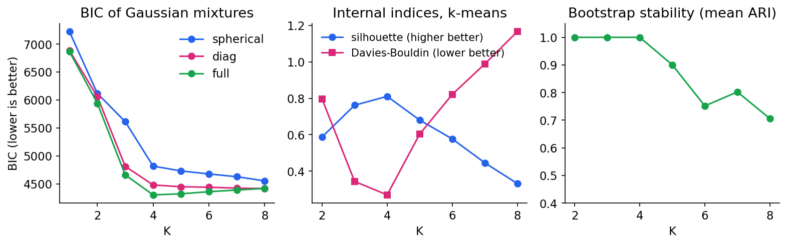
BIC picks the true with full covariances (the shear made the clusters elliptical, so spherical and diagonal models need extra components). AIC slightly prefers : its lighter penalty lets a fifth component buy a small likelihood gain. Neither criterion is “right” in general; both assume the model family is adequate, and for non-Gaussian clusters BIC will happily use several Gaussians to describe one curved group. If the goal is density estimation, that is fine; if each component is supposed to be one semantic group, it is not.
Other heuristics
The elbow method plots k-means against and looks for a bend; always decreases, so the bend is subjective. The silhouette and stability approaches in the next section give alternatives. A Bayesian treatment can also start with more components than needed and let a prior on the mixing weights switch the unnecessary ones off; Bishop works through this for a variational Gaussian mixture [2].
Cluster validity: is the clustering any good?
Plain version. Without labels, “good” has to be defined: tight and well separated (internal indices), agreeing with some trusted reference (external indices), or reproducible when the data are perturbed (stability). Theodoridis and Koutroumbas devote Chapter 16 to these questions [1]; PR 09 returns to validation in the supervised setting.
Internal indices
Silhouette [14]. For point in cluster , let be its mean distance to the other points in , and the smallest mean distance from to the points of any other cluster. Then
near means sits well inside its cluster; near , on a boundary; negative, probably in the wrong cluster. The mean silhouette over all points summarizes a partition, and the per-point silhouette plot shows which clusters are weak.
Davies–Bouldin [15]. Let be the average distance of cluster ‘s points to its centroid , and . Then
the average “worst-case similarity” of each cluster to another. Lower is better.
Calinski–Harabasz [16]. With between-cluster scatter and within-cluster scatter ( is the overall mean),
a variance-ratio statistic. Higher is better.
All three reward compact, convex, well-separated clusters in the chosen geometry. They will rate k-means’ wrong answer on the two moons higher than the correct curved answer. They measure agreement with an assumed cluster shape, not semantic correctness.
External indices
When reference labels exist (for benchmarking, or for a separate held-out annotation), compare partitions with permutation-invariant indices.
Adjusted Rand index (ARI) [17]. The Rand index counts the fraction of point pairs on which two partitions agree (both “same cluster” or both “different cluster”). ARI subtracts the value expected under random labelings with the same cluster sizes and rescales:
so random partitions score about and identical partitions (up to relabeling) score .
Normalized mutual information (NMI). Treat the two labelings and as random variables over points; then
with mutual information and entropies (the arithmetic-mean normalization shown is scikit-learn’s default; other normalizations exist). Vinh, Epps and Bailey [18] showed that unadjusted NMI is biased upward when the number of clusters is large relative to , and recommend chance-adjusted versions such as adjusted mutual information (AMI).
If the reference labels were used to tune the algorithm or , they are no longer an independent check.
Stability
Refit the clustering on bootstrap samples or perturbed data and compare each new partition with the original on the same points, using ARI. A that gives unstable partitions is suspect. But stability is necessary, not sufficient: merging two nearby blobs is perfectly reproducible (Figure 6, right, ), and a stable partition can still reflect an irrelevant factor such as the camera or the lighting.
Code: validity indices and stability
Code · Python · 30 lines
import numpy as np
from sklearn.datasets import make_blobs
from sklearn.cluster import KMeans
from sklearn.metrics import (silhouette_score, davies_bouldin_score,
                             calinski_harabasz_score, adjusted_rand_score,
                             normalized_mutual_info_score)

X, truth = make_blobs(n_samples=600, centers=4, cluster_std=1.0, random_state=7)
print(" K  silhouette(+)  Davies-Bouldin(-)  Calinski-Harabasz(+)")
for K in range(2, 8):
    z = KMeans(K, n_init=10, random_state=0).fit_predict(X)
    print(f"{K:2d}  {silhouette_score(X, z):12.3f}  {davies_bouldin_score(X, z):17.3f}"
          f"  {calinski_harabasz_score(X, z):20.1f}")

z = KMeans(4, n_init=10, random_state=0).fit_predict(X)
print("external ARI:", round(adjusted_rand_score(truth, z), 3),
      " NMI:", round(normalized_mutual_info_score(truth, z), 3))
perm = np.array([2, 0, 3, 1])[z]                       # relabel clusters
print("ARI after relabelling:", round(adjusted_rand_score(truth, perm), 3))

# stability: refit on bootstrap samples, compare on the original points
rng = np.random.default_rng(1)
for K in [3, 4, 5, 6]:
    base = KMeans(K, n_init=10, random_state=0).fit(X)
    scores = []
    for b in range(10):
        idx = rng.integers(0, len(X), len(X))
        boot = KMeans(K, n_init=10, random_state=b).fit(X[idx])
        scores.append(adjusted_rand_score(base.predict(X), boot.predict(X)))
    print(f"K={K}: bootstrap stability (mean ARI) = {np.mean(scores):.3f}")
Output
 K  silhouette(+)  Davies-Bouldin(-)  Calinski-Harabasz(+)
 2         0.588              0.796                 850.9
 3         0.762              0.343                2235.5
 4         0.811              0.270                7641.8
 5         0.680              0.603                6341.0
 6         0.577              0.821                5620.2
 7         0.446              0.988                5304.4
external ARI: 1.0  NMI: 1.0
ARI after relabelling: 1.0
K=3: bootstrap stability (mean ARI) = 1.000
K=4: bootstrap stability (mean ARI) = 1.000
K=5: bootstrap stability (mean ARI) = 0.858
K=6: bootstrap stability (mean ARI) = 0.699
On these well-separated blobs every internal index agrees on , and the external indices confirm a perfect match regardless of how the clusters are numbered. Real data are rarely this kind: indices frequently disagree, and the disagreement is informative, because it tells you the data do not have one unambiguous cluster structure at the chosen scale.
Modern view
Plain version. The algorithms in this chapter are decades old and still everywhere. What changed is the representation: today we usually cluster learned embeddings rather than raw pixels or hand-made descriptors, and deep networks are sometimes trained by clustering.
Surveys worth reading
- Xu and Wunsch, “Survey of clustering algorithms” (2005) [19] is the classic broad survey from a pattern-recognition and neural-network viewpoint. It reviews proximity measures, then organizes algorithms into hierarchical, squared-error (k-means family), mixture-density, graph-theoretic, fuzzy, neural (self-organizing maps, adaptive resonance), kernel, sequential-data, large-scale and high-dimensional methods, and closes with cluster validity. It is a good map of the classical landscape.
- Jain, “Data clustering: 50 years beyond K-means” (2010) [20] is a shorter, opinionated overview. Its main messages remain current: there is no universally best algorithm; the representation and the definition of a cluster matter more than the algorithm; the number of clusters and validity are open questions; and side information (pairwise constraints, semi-supervised clustering) and clustering ensembles are valuable directions.
- Ikotun et al., “K-means clustering algorithms: A comprehensive review, variants analysis, and advances in the era of big data” (2023) [21] reviews the many k-means variants: initialization (including k-means++), automatic choice of , handling of mixed or high-dimensional data, and scalable and distributed implementations.
- Zhou et al., “A comprehensive survey on deep clustering: Taxonomy, challenges, and future directions” (ACM Computing Surveys, 2024) [22] organizes deep clustering by how the representation-learning module and the clustering module interact: multi-stage methods (learn features, then cluster), iterative methods (alternate pseudo-labels and feature learning), generative methods (latent-variable models such as mixture-prior autoencoders), and simultaneous methods (optimize both jointly). It also discusses benchmarks, metrics and applications.
- Ren et al., “Deep clustering: A comprehensive survey” (IEEE TNNLS, 2025) [23] organizes the field by data source and prior knowledge: single-view, semi-supervised, multi-view and transfer deep clustering. Read together with [22], it shows how wide the deep-clustering design space has become.
From visual words to self-labeling
Two influential vision papers show how classical clustering became a training signal. DeepCluster [24] alternates between running k-means on the features of a convolutional network and training that network to predict the cluster assignments as pseudo-labels; repeated over the whole data set, this learns useful features from unlabeled images. SCAN [25] separates representation learning from clustering: it first learns features with a self-supervised pretext task, then mines each image’s nearest neighbors in that feature space and trains a clustering head so that neighbors receive the same cluster, followed by a self-labeling refinement. Both are applications of the ideas in this chapter (k-means as quantization, neighborhoods as evidence of similarity) to learned representations; ML 06 explains where such representations come from.
State of practice (2023–2026) and open problems
In current practice, a common recipe for grouping images is: extract embeddings from a pretrained (often self-supervised) encoder, optionally reduce dimension, then run k-means, a Gaussian mixture or HDBSCAN, and validate on a labeled subset. The chapter’s warnings apply unchanged:
- The representation defines similarity. Embeddings trained for one purpose may cluster by style, background or camera rather than by the category you care about.
- and validity remain open. Information criteria assume the model family; internal indices assume a shape; external indices need labels. No survey above claims a general solution.
- Evaluation of deep clustering usually relies on labeled benchmarks and permutation-invariant scores such as clustering accuracy after optimally matching clusters to classes, NMI and ARI [22]. Those scores measure agreement with one chosen labeling, not the “true” structure.
- Scale and imbalance. Long-tailed data, many small clusters, and streaming data stress both classical and deep methods; [21] and [22] list these as active problems.
Key takeaways
- Clustering is defined by its notion of similarity. Features, scaling and distance are modeling decisions made before any algorithm runs.
- K-means (Lloyd) alternates nearest-center assignment and mean update; decreases monotonically to a local minimum. k-means++ seeding gives and far fewer bad runs; use several restarts anyway.
- Linkage defines hierarchical clustering: single linkage chains along thin bridges, complete and Ward prefer compact groups. The dendrogram must still be cut.
- DBSCAN defines clusters as density-connected regions, finds arbitrary shapes and labels noise; comes from the k-distance curve, and HDBSCAN handles varying density.
- EM for Gaussian mixtures follows from the complete-data log-likelihood: E step responsibilities, M step weighted means and covariances, via a Lagrange multiplier. The ELBO decomposition proves monotone improvement; singularities and label switching need explicit care; k-means is the hard, isotropic limit.
- BIC and AIC trade fit against parameter count; covariance type is part of the choice.
- Internal indices (silhouette, Davies–Bouldin, Calinski–Harabasz) reward an assumed geometry; external indices (ARI, NMI) need independent labels; stability is necessary but not sufficient.
Exercises
- Lloyd’s algorithm never increases . Prove that both the assignment step and the update step cannot increase , and use this to argue that the algorithm terminates. What goes wrong with the termination argument if ties are broken randomly?
Hint
The assignment step minimizes each term separately; the update step uses . There are at most partitions. With random tie-breaking, two partitions of equal could alternate forever; a fixed rule (for example, keep the current cluster on ties) prevents that.
- k-means++ by hand. One-dimensional data are and . The first seed is . Compute the probability that each point becomes the second seed. Then compare with uniform sampling of the second seed.
Hint
values are , summing to . So and ; together about . Under uniform sampling the second seed lands in the right-hand group with probability only (or if the first seed is excluded).
- The M step for a 1-D mixture. For a one-dimensional two-component mixture with variances , derive the M-step update of from directly, without matrix calculus. Then show that if a component’s responsibilities concentrate on one point (that is, for that point and for the others), the update drives toward . What does scikit-learn’s
reg_covardo about it?
Hint
Differentiate with respect to to get . With all weight on one point, and the sum is zero. reg_covar adds a small constant to the diagonal after each M step, so the variance stays bounded away from zero.
- Counting parameters. For local descriptors with and components, count the free parameters of a GMM with full, diagonal and spherical covariances. With descriptors, how large is the BIC penalty in each case?
Hint
Full: . Diagonal: . Spherical: . Multiply by . The full model has to improve by roughly over the diagonal one just to break even.
- When indices mislead. Run k-means with and DBSCAN on the two-moons data from the comparison code. Compute the silhouette score of each partition and their ARI against the generating labels. Explain the disagreement in terms of what each index measures.
Hint
Silhouette is computed from Euclidean distances and favors convex, separated groups, so the k-means cut usually scores higher than the two moons even though its ARI is about 0.26 versus 1.0 for DBSCAN. Internal indices encode a shape assumption; the “right” answer here is defined by connectivity.
- Stability is not truth. Generate four Gaussian blobs where two are very close (for example centers and with standard deviation ). Compute bootstrap stability for and . Which is more stable? Which matches the generating process? What extra information would settle it?
Hint
Merging the close pair is very reproducible, so can be as stable as or more stable than . The generating process has four groups, but whether they should be separated depends on the task. Domain knowledge, a labeled subset, or a density-based criterion such as BIC on a GMM gives additional evidence.
References
-
S. Theodoridis and K. Koutroumbas, Pattern Recognition, 4th ed., Academic Press, 2009, Ch. 11–16 (clustering basic concepts, sequential, hierarchical, function-optimization and graph-based algorithms, cluster validity). doi
-
C. M. Bishop, Pattern Recognition and Machine Learning, Springer, 2006, Ch. 9 (k-means, mixtures of Gaussians, EM, the general EM algorithm). book page
-
S. P. Lloyd, “Least squares quantization in PCM,” IEEE Transactions on Information Theory, vol. 28, no. 2, pp. 129–137, 1982. doi
-
J. MacQueen, “Some methods for classification and analysis of multivariate observations,” in Proc. Fifth Berkeley Symposium on Mathematical Statistics and Probability, vol. 1, pp. 281–297, 1967. Project Euclid
-
D. Arthur and S. Vassilvitskii, “k-means++: The advantages of careful seeding,” in Proc. 18th Annual ACM-SIAM Symposium on Discrete Algorithms (SODA), 2007, pp. 1027–1035. pdf
-
D. Sculley, “Web-scale k-means clustering,” in Proc. 19th International Conference on World Wide Web (WWW), 2010, pp. 1177–1178. doi
-
J. H. Ward, “Hierarchical grouping to optimize an objective function,” Journal of the American Statistical Association, vol. 58, pp. 236–244, 1963. doi
-
M. Ester, H.-P. Kriegel, J. Sander and X. Xu, “A density-based algorithm for discovering clusters in large spatial databases with noise,” in Proc. 2nd International Conference on Knowledge Discovery and Data Mining (KDD), 1996. pdf
-
R. J. G. B. Campello, D. Moulavi and J. Sander, “Density-based clustering based on hierarchical density estimates,” in Advances in Knowledge Discovery and Data Mining (PAKDD), LNCS, 2013, pp. 160–172. doi
-
U. von Luxburg, “A tutorial on spectral clustering,” Statistics and Computing, vol. 17, pp. 395–416, 2007. doi
-
A. P. Dempster, N. M. Laird and D. B. Rubin, “Maximum likelihood from incomplete data via the EM algorithm,” Journal of the Royal Statistical Society: Series B, vol. 39, no. 1, pp. 1–22, 1977. doi
-
G. Schwarz, “Estimating the dimension of a model,” The Annals of Statistics, vol. 6, no. 2, 1978. doi
-
H. Akaike, “A new look at the statistical model identification,” IEEE Transactions on Automatic Control, vol. 19, no. 6, pp. 716–723, 1974. doi
-
P. J. Rousseeuw, “Silhouettes: A graphical aid to the interpretation and validation of cluster analysis,” Journal of Computational and Applied Mathematics, vol. 20, pp. 53–65, 1987. doi
-
D. L. Davies and D. W. Bouldin, “A cluster separation measure,” IEEE Transactions on Pattern Analysis and Machine Intelligence, vol. PAMI-1, no. 2, pp. 224–227, 1979. doi
-
T. Caliński and J. Harabasz, “A dendrite method for cluster analysis,” Communications in Statistics, vol. 3, no. 1, pp. 1–27, 1974. doi
-
L. Hubert and P. Arabie, “Comparing partitions,” Journal of Classification, vol. 2, pp. 193–218, 1985. doi
-
N. X. Vinh, J. Epps and J. Bailey, “Information theoretic measures for clusterings comparison: Variants, properties, normalization and correction for chance,” Journal of Machine Learning Research, vol. 11, pp. 2837–2854, 2010. JMLR
-
R. Xu and D. Wunsch II, “Survey of clustering algorithms,” IEEE Transactions on Neural Networks, vol. 16, no. 3, pp. 645–678, 2005. doi
-
A. K. Jain, “Data clustering: 50 years beyond K-means,” Pattern Recognition Letters, vol. 31, no. 8, pp. 651–666, 2010. doi
-
A. M. Ikotun, A. E. Ezugwu, L. Abualigah, B. Abuhaija and J. Heming, “K-means clustering algorithms: A comprehensive review, variants analysis, and advances in the era of big data,” Information Sciences, vol. 622, pp. 178–210, 2023. doi
-
S. Zhou, H. Xu, Z. Zheng, J. Chen, Z. Li, J. Bu, J. Wu, X. Wang, W. Zhu and M. Ester, “A comprehensive survey on deep clustering: Taxonomy, challenges, and future directions,” ACM Computing Surveys, vol. 57, no. 3, pp. 1–38, 2024 (arXiv:2206.07579). doi
-
Y. Ren, J. Pu, Z. Yang, J. Xu, G. Li, X. Pu, P. S. Yu and L. He, “Deep clustering: A comprehensive survey,” IEEE Transactions on Neural Networks and Learning Systems, vol. 36, no. 4, pp. 5858–5878, 2025 (arXiv:2210.04142). doi
-
M. Caron, P. Bojanowski, A. Joulin and M. Douze, “Deep clustering for unsupervised learning of visual features,” in Proc. European Conference on Computer Vision (ECCV), LNCS, 2018, pp. 139–156. doi
-
W. Van Gansbeke, S. Vandenhende, S. Georgoulis, M. Proesmans and L. Van Gool, “SCAN: Learning to classify images without labels,” in Proc. European Conference on Computer Vision (ECCV), LNCS, 2020, pp. 268–285. doi
-
scikit-learn developers, “GaussianMixture,” API documentation, accessed 2026-11-05. documentation
Check your understanding
This tutorial has 6 exercises. Can you solve them without opening the hints?
Go to the exercises ↑Next PR 08 · Approximate Inference and Bayesian Model Complexity · 28 min