PR 03 · Linear Models for Regression and Classification
Needs: PR 02 · Density Estimation and Bayesian Learning, ML 01C · Numerical Computation and Gradient Checks
Navigate: this page and this track: Navigate: this page and this track
On this page
- What you’ll learn1 min
- The big picture1 min
- Linear discriminant functions2 min
- Least squares and ridge regression1 min
- Least squares for classification1 min
- Fisher’s linear discriminant2 min
- The perceptron2 min
- Logistic regression2 min
- Support vector machines: maximum margin3 min
- One picture: linear classifiers as losses2 min
- Modern view3 min
- Key takeaways1 min
- Exercises2 min
- References
Pattern Recognition
Explore this chapter 1 interactive experiment
Fit polynomial basis functions with ridge regression and separate training error from recovery of the underlying function.
What you’ll learn
- Read the geometry of a linear discriminant (weight vector, bias, signed distance) and the pitfalls of building multiclass classifiers from two-class ones.
- Derive least squares, ridge regression and their Bayesian interpretation, and see why least squares is a fragile classifier.
- Derive Fisher’s linear discriminant and connect it to Gaussian LDA from PR 01.
- Train a perceptron, prove its convergence theorem, and explain why it can stop at any separating line.
- Fit logistic regression by Newton’s method, and explain why separable data push its weights to infinity.
- Derive the maximum-margin SVM, its Lagrangian dual and its support vectors, and see all of these methods as different losses on the same linear score.
The big picture
Linear models are the first serious classifiers in every pattern-recognition course, and they remain the first thing to try on a new representation. If a straight boundary separates two categories in feature space, a large nonlinear classifier may add cost without useful accuracy. If a linear baseline fails, its errors help identify missing features or nonlinear structure. In modern deep learning, the final layer of almost every classifier is a linear model on learned features, and “how well does a linear classifier do on these features?” is the standard test of a representation.
A linear score is . The feature map might contain raw intensities, squared values, gradients or a frozen neural embedding. “Linear” refers to the parameters and , not necessarily to the original measurement : with a linear model draws a curved boundary in . This chapter follows Duda, Hart and Stork [1, Ch. 5], Bishop [2, Ch. 3–4, 7] and Theodoridis and Koutroumbas [3, Ch. 3], with Hastie et al. [4] for the statistical view. Kernels, which make implicit and very rich, are the topic of PR 04.
Linear discriminant functions
Plain version. A two-class linear classifier is a flat cut through feature space: a line in 2-D, a plane in 3-D, a hyperplane in general. The weight vector says which way the cut faces; the bias says where it sits.
Precise version. For two classes, decide if and otherwise. The decision boundary is a hyperplane . Three facts follow from the geometry of linear classifiers [1, 2, 3]:
- is normal to : for two points on , .
- The signed distance from any to is . So is proportional to how far, and on which side, lies.
- For , the ordinary distance from the origin to is . Its signed distance under the convention above is ; the closest point on is . The bias shifts the plane without rotating it.
It is convenient to absorb the bias by augmenting the input with a constant: and , so that . We do this silently in code. With labels , a sample is correctly classified exactly when its functional margin is positive. Every method below can be written in terms of this quantity.
More than two classes. Two-class machines can be combined in two obvious ways: one-versus-rest ( classifiers, each separating one class from all others) and one-versus-one ( classifiers, one per pair, followed by voting). Both can leave regions of input space where the votes are ambiguous [2, Section 4.1.2]. The clean solution is a linear machine: one discriminant per class, , and assign to the class with the largest score. Its decision regions are always convex and simply connected, because if and both have largest, so does every point between them (each is linear along the segment). The Gaussian LDA of PR 01, multiclass logistic regression and the final layer of a neural network are all linear machines.
Least squares and ridge regression
Plain version. For predicting a quantity, choose the weights that make the squared prediction errors as small as possible. If there are too many weights for the data, also penalize large weights.
Precise version. Let row of the design matrix be the feature vector , including a constant coordinate for the intercept, and let hold the targets. Least squares minimizes
whose gradient vanishes at the normal equations . Forming squares the 2-norm condition number for a full-column-rank design, and explicitly inverting it is unnecessary; QR- or SVD-based solvers (np.linalg.lstsq) handle near-dependent columns more reliably. Assuming independent Gaussian noise of common variance on the targets, this objective equals the negative log-likelihood up to a positive scale and an additive constant, so least squares is the maximum-likelihood estimate (PR 02). The noise assumption explains the statistical interpretation; it does not make squared error suitable for every target.
Ridge regression [8] adds a penalty , giving
The matrix on the left is invertible for any , even when . Usually the intercept is excluded from the penalty. Feature scaling matters, because the same penalty has different effects on coordinates measured in different units; fit scaling statistics on training data only.
A Bayesian connection
With a Gaussian prior (precision ) and Gaussian noise of precision , the posterior over weights is Gaussian with covariance and mean [2, Section 3.3]
For a new feature vector , the predictive distribution is
The first variance term is observation noise; the second expresses uncertainty about the weights, which is larger along feature directions that the training data rarely visited. The posterior mean equals the ridge solution with : ridge is a MAP estimate, the same story as the Gaussian mean in PR 02.
Least squares for classification
Plain version. You can treat class labels as numbers ( and , or one-hot vectors) and fit them with least squares. It is fast and has a closed form, but it is the wrong tool: it punishes points for being too correct.
Precise version. For classes, encode the targets as one-hot vectors and fit a linear machine by least squares, , then classify by the largest output. For two classes with suitable target values ( for class 1 and for class 0), the least-squares direction is exactly Fisher’s direction derived in the next section [2, Section 4.1.5], so the method is not unreasonable.
It has two well-known failure modes:
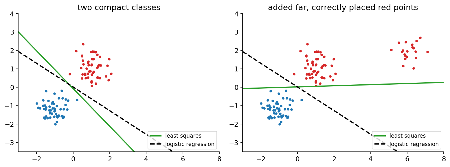
- Sensitivity to points far on the correct side. Squared error penalizes for a target of as severely as . Figure 1 adds twenty red points that are correctly classified but far away; least squares rotates its boundary to reduce their “error” and starts misclassifying blue points. Logistic regression barely moves.
- Masking with three or more classes. When classes lie roughly along a line, the output for the middle class can be dominated everywhere by one of its neighbors, so the middle class is never predicted [4, Section 4.2].
In probabilistic terms, the Gaussian noise model behind least squares is simply wrong for binary targets. The remedy is to use a loss designed for classification, which the rest of the chapter does.
Fisher’s linear discriminant
Plain version. Project all points onto one line and look at the two classes’ 1-D histograms. A good line makes the class means far apart and each class narrow. Fisher’s direction is the line that maximizes this ratio.
Precise version. Fisher [5] proposed choosing a projection that maximizes the separation of the projected class means relative to the spread within each class. Let be the class means. The projected means are , and the projected within-class scatter of class is , with . Fisher’s criterion is
where
are the between-class and within-class scatter matrices. does not depend on the length of , only on its direction.
Derivation. Setting the gradient of the ratio to zero gives
Both bracketed terms are scalars. Moreover always points along . Hence , and since only the direction matters,
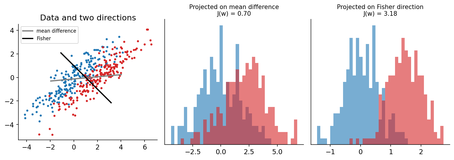
If is a multiple of the identity (isotropic, uncorrelated classes), Fisher’s direction is just the mean difference. Otherwise rotates it away from directions in which the classes are spread out. Figure 2 shows the effect for two elongated, correlated classes: projecting on the mean difference gives heavily overlapping histograms (), while Fisher’s direction separates them well ().
Relationship with Gaussian LDA. Fisher’s criterion makes no distributional assumption; it is a criterion for a representation. Yet its direction coincides with the Gaussian LDA direction of PR 01 when is (proportional to) the pooled within-class covariance. The two differ only in the threshold: Fisher leaves the cut point on the projected axis open, while Gaussian LDA fixes it from the class means and priors. So “LDA” is used for both. (In topic modelling, LDA also means latent Dirichlet allocation, which is unrelated.) Fisher projections do not by themselves provide calibrated probabilities.
More than two classes. With classes and overall mean , define and . The projection that maximizes the multiclass criterion is spanned by the leading eigenvectors of [1, 2]. Because is a sum of rank-one terms constrained by the overall mean, its rank is at most , so Fisher can produce at most useful features. This is the supervised dimensionality reduction of PR 05.
Code: Fisher’s direction
Code · Python · 21 lines
import numpy as np
from sklearn.discriminant_analysis import LinearDiscriminantAnalysis

rng = np.random.default_rng(2)
cov = np.array([[3.0, 2.4], [2.4, 2.4]])
X0 = rng.multivariate_normal([0, 0], cov, 200)
X1 = rng.multivariate_normal([2, 0], cov, 200)
m0, m1 = X0.mean(0), X1.mean(0)
S_W = np.cov(X0.T) + np.cov(X1.T)       # within-class scatter (per-class covariances)
w = np.linalg.solve(S_W, m1 - m0)                          # Fisher direction

def J(v):                       # Fisher criterion for two classes
    return (v @ (m1 - m0)) ** 2 / (v @ S_W @ v)

lda = LinearDiscriminantAnalysis().fit(np.vstack([X0, X1]), np.repeat([0, 1], 200))
cos = w @ lda.coef_[0] / np.linalg.norm(w) / np.linalg.norm(lda.coef_[0])
angles = np.linspace(0, np.pi, 3601)
best = max(J(np.array([np.cos(a), np.sin(a)])) for a in angles)
print(f"J(mean difference) = {J(m1 - m0):.4f}, J(Fisher) = {J(w):.4f}, "
      f"grid maximum = {best:.4f}")
print(f"cosine between Fisher direction and LDA coef_: {cos:.6f}")
The closed form attains the grid maximum (), more than four times the mean-difference value (), and its direction agrees with scikit-learn’s Gaussian LDA coefficients to six decimals (cosine ).
The perceptron
Plain version. Start with any line. Go through the training points; whenever one is on the wrong side, nudge the line towards classifying it correctly. If the classes can be separated by a line, this process is guaranteed to stop.
Precise version. Rosenblatt’s perceptron [6] uses labels and augmented features . It minimizes the perceptron criterion
where is the set of misclassified samples (those with ). Each term is non-negative, and exactly when every sample is correctly classified. Stochastic gradient descent on one misclassified sample at a time gives the update
With initialized at zero, the learning rate only rescales and does not change the sequence of decisions, so is common. The IP 13 perceptron section presents the same rule in the language of image patterns and connects it to multilayer networks.
Convergence theorem. Suppose the data are linearly separable with margin : some unit vector satisfies for all . Let . Then the perceptron (started at ) makes at most updates. The proof takes three lines. After updates:
- each update adds to , so ;
- each update happens on a mistake, where , so , hence ;
- by Cauchy–Schwarz, , so .
The bound does not depend on the number of samples or the dimension, only on how “fat” the gap between the classes is relative to the data’s size.
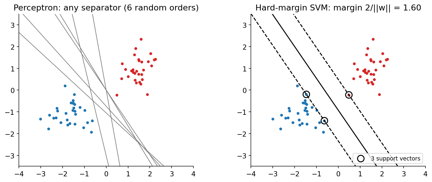
Limitations. If the classes overlap, the perceptron never stops; the weights keep cycling (variants that keep the best weights seen so far are a common practical fix). Even when it converges, it stops at the first separating hyperplane it reaches, which depends on initialization and data order (Figure 3, left). And its score is not a probability. In terms of losses, the perceptron uses , which is zero for any correct classification, however marginal. Both logistic regression and the SVM fix this by asking for more than “just barely correct”.
Code: perceptron updates versus the bound
Code · Python · 35 lines
import numpy as np
from sklearn.svm import SVC

rng = np.random.default_rng(1)
X = np.vstack([rng.normal([-1.0, -0.7], 0.6, (30, 2)),
               rng.normal([1.0, 0.7], 0.6, (30, 2))])
y = np.r_[-np.ones(30), np.ones(30)]
Phi = np.c_[X, np.ones(len(X))]          # augmented features (bias as last weight)

def perceptron(Phi, y, rng, max_epochs=1000):
    w, updates = np.zeros(Phi.shape[1]), 0
    for epoch in range(max_epochs):
        errors = 0
        for i in rng.permutation(len(y)):
            if y[i] * (w @ Phi[i]) <= 0:  # misclassified or on the boundary
                w += y[i] * Phi[i]        # learning rate 1 (scale is irrelevant)
                errors += 1
        updates += errors
        if errors == 0:
            return w, updates
    return w, updates

runs = [perceptron(Phi, y, np.random.default_rng(s)) for s in range(200)]
updates = np.array([u for _, u in runs])
print(f"updates over 200 random orders: mean {updates.mean():.1f}, "
      f"max {updates.max()}")
print("all runs separate the data:",
      all(np.all(np.sign(Phi @ w) == y) for w, _ in runs))

# convergence bound (R / gamma)^2, with gamma from the max-margin separator
svm = SVC(kernel="linear", C=1e6).fit(X, y)
u = np.r_[svm.coef_[0], svm.intercept_[0]]
gamma = np.min(y * (Phi @ u)) / np.linalg.norm(u)
R = np.max(np.linalg.norm(Phi, axis=1))
print(f"bound (R/gamma)^2 = {(R / gamma) ** 2:.1f}")
Over 200 random presentation orders the perceptron needs on average updates (at most ), and every run separates the data. The worst-case bound is : it is a guarantee, not a prediction. The bound needs a valid margin ; we take it from a hard-margin SVM (the subject of the SVM section below). Because the SVM does not penalize the bias, the true maximum margin in the augmented space may be slightly larger, which would give a slightly tighter bound.
Logistic regression
Plain version. Instead of a hard yes/no, output a probability by squashing the linear score through an S-shaped curve. Fit the weights so that the probabilities assigned to the true labels are as high as possible.
Precise version. With labels , binary logistic regression [7] models
The score is the log-odds . This form is not arbitrary. PR 01 showed that for Gaussian classes with a shared covariance the posterior is exactly with ; the same holds for many other class-conditional families. Logistic regression keeps the functional form of that posterior but fits directly, with parameters instead of the of the Gaussian model. Ng and Jordan [18] analysed this generative–discriminative trade-off (PR 02).
Training. The negative log-likelihood of the Bernoulli model is the cross-entropy
Because , its gradient and Hessian are remarkably simple [2, Section 4.3]:
The gradient has the same “prediction minus target, times input” form as least squares. is positive semidefinite, so is convex and has no spurious local minima. Newton’s method, , can be rewritten as a weighted least-squares problem with weights that change every iteration: iteratively reweighted least squares (IRLS). In code, compute losses from logits with a stable formula such as np.logaddexp(0, z) rather than taking logarithms of rounded probabilities.
Separable data. If a hyperplane separates the training classes, scaling up pushes every closer to its label, so keeps decreasing towards zero and the unregularized solution does not exist: . In practice, always regularize, e.g. add (scikit-learn’s C is ). Remarkably, how the weights diverge is well defined: plain gradient descent on separable data converges in direction to the maximum-margin SVM solution [19], which the Modern view returns to.
Multiclass. Replace the sigmoid with the softmax and the cross-entropy with its -class version. This is a linear machine with probabilistic outputs, and it is exactly the last layer plus loss of a standard neural classifier. Probability outputs are not automatically calibrated under label noise or distribution shift (PR 01).
Code: Newton’s method (IRLS) and separable data
Code · Python · 27 lines
import numpy as np
from sklearn.linear_model import LogisticRegression

rng = np.random.default_rng(0)
X = np.vstack([rng.normal(-1, 1, (100, 2)), rng.normal(1, 1, (100, 2))])
y = np.r_[np.zeros(100), np.ones(100)]
Phi = np.c_[np.ones(len(X)), X]

def nll(w, lam):
    z = Phi @ w
    # log(1 + e^z) - y z, written stably with logaddexp
    return np.sum(np.logaddexp(0, z) - y * z) + 0.5 * lam * np.sum(w[1:] ** 2)

# Newton's method (iteratively reweighted least squares)
lam, w = 1.0, np.zeros(3)
for it in range(20):
    p = 1 / (1 + np.exp(-(Phi @ w)))
    grad = Phi.T @ (p - y) + lam * np.r_[0, w[1:]]
    H = Phi.T @ (Phi * (p * (1 - p))[:, None]) + lam * np.diag([0, 1, 1])
    step = np.linalg.solve(H, grad)
    w -= step
    if np.linalg.norm(step) < 1e-10:
        break
sk = LogisticRegression(C=1 / lam, tol=1e-10, max_iter=1000).fit(X, y)
print(f"Newton converged in {it + 1} iterations, loss {nll(w, lam):.4f}")
print("Newton:      ", np.round(w, 4))
print("scikit-learn:", np.round(np.r_[sk.intercept_, sk.coef_[0]], 4))
Newton’s method converges in iterations to the same weights as scikit-learn, for (intercept, , ). The penalty excludes the intercept, matching scikit-learn’s convention.
The next snippet runs plain gradient descent on unregularized logistic loss for data that a line through the origin separates. It tracks the weight norm and the cosine between and the max-margin direction.
Code · Python · 20 lines
import numpy as np
from sklearn.svm import LinearSVC

rng = np.random.default_rng(1)
X = np.vstack([rng.normal([2.0, 1.0], 0.6, (40, 2)),
               rng.normal([-2.0, -1.0], 0.6, (40, 2))])
y = np.r_[np.ones(40), -np.ones(40)]              # separable through the origin

# max-margin direction without bias (hard margin approximated by large C)
svm = LinearSVC(fit_intercept=False, loss="hinge", C=1e4, max_iter=200000).fit(X, y)
u = svm.coef_[0] / np.linalg.norm(svm.coef_[0])

w, lr = np.zeros(2), 0.1
for t in range(1, 100001):
    m = y * (X @ w)
    grad = -(X * (y / (1 + np.exp(m)))[:, None]).mean(0)   # logistic loss gradient
    w -= lr * grad
    if t in (10, 100, 1000, 10000, 100000):
        print(f"step {t:6d}: ||w|| = {np.linalg.norm(w):6.2f}, "
              f"cos(w, SVM) = {w @ u / np.linalg.norm(w):.5f}")
The norm grows without bound but only slowly ( after 10 steps, after ), while the cosine with the SVM direction creeps from to . This is the logarithmically slow convergence to the max-margin direction predicted by Soudry et al. [19].
Support vector machines: maximum margin
Plain version. Among all lines that separate the classes, pick the one with the widest empty “street” around it. Only the points on the edges of the street matter; move any other point (without crossing the street) and the answer does not change.
Precise version. Use labels and score (bias kept separate here). For a separating hyperplane, the distance of to the boundary is . Since and define the same plane, fix the scale so that the closest points satisfy (the canonical form). The margin on each side is then and the street has width . Maximizing it is equivalent to the convex quadratic program [9, 10]
Lagrangian and dual. Introduce multipliers , one per constraint:
Setting and gives
Substituting back eliminates and and leaves the dual problem
Three consequences matter [2, 11]:
- Support vectors. The Karush–Kuhn–Tucker conditions include complementary slackness, . So only for points exactly on the margin. These are the support vectors; all other points have and can be removed without changing the solution. The bias follows from any support vector : (average over all of them for numerical stability).
- Sparsity of the prediction. depends only on support vectors .
- Only inner products. The data appear in the dual and in the prediction only through inner products . Replacing them with a kernel gives a nonlinear SVM without ever computing . That is the kernel trick, developed in PR 04.
Soft margin and the hinge loss. Real classes overlap, so the constraints cannot all hold. Cortes and Vapnik [10] added slack variables , constraints , and a penalty . At the optimum , so the soft-margin SVM is equivalent to the unconstrained problem
The second term is the hinge loss: zero for points beyond the margin, linear inside it and on the wrong side. In the dual the only change is a box constraint . So a linear SVM is “ridge-regularized hinge-loss minimization”, directly comparable to regularized logistic regression. The roles of , kernel bandwidth and feature scaling, and the fact that an SVM score is not a probability, are treated in PR 04.
Code: the dual in practice
This check fits a (nearly) hard-margin linear SVM and verifies the dual relations numerically: , , and on the support vectors.
Code · Python · 19 lines
import numpy as np
from sklearn.svm import SVC

rng = np.random.default_rng(7)
X = np.vstack([rng.normal([-1.5, -1.0], 0.6, (30, 2)),
               rng.normal([1.5, 1.0], 0.6, (30, 2))])
y = np.r_[-np.ones(30), np.ones(30)]

svm = SVC(kernel="linear", C=1e6).fit(X, y)          # huge C ~ hard margin
alpha_y = svm.dual_coef_[0]                          # alpha_n * y_n for SVs
w_dual = alpha_y @ svm.support_vectors_              # w = sum_n alpha_n y_n x_n
f = X @ svm.coef_[0] + svm.intercept_[0]

print("support vectors:", len(svm.support_), "of", len(y))
print("w from dual:", np.round(w_dual, 4), " coef_:", np.round(svm.coef_[0], 4))
print("sum_n alpha_n y_n =", round(float(alpha_y.sum()), 8))
print("y f(x) on support vectors:", np.round(y[svm.support_] * f[svm.support_], 4))
print("smallest y f(x) over all points:", round(float(np.min(y * f)), 4))
print("margin width 2/||w|| =", round(2 / np.linalg.norm(svm.coef_[0]), 4))
Only of the points are support vectors (the circled points in Figure 3). The weight vector rebuilt from the dual coefficients matches coef_ exactly, the dual coefficients sum to zero, the support vectors sit at (to solver tolerance), no point is inside the margin, and the margin width is . scikit-learn’s SVC wraps LIBSVM [16]; for large sparse problems, LinearSVC and LogisticRegression(solver="liblinear") use LIBLINEAR [14], and stochastic sub-gradient solvers such as Pegasos [15] scale to very large datasets.
One picture: linear classifiers as losses
Plain version. All the methods in this chapter score a point with the same linear function. They differ in how much they charge for each value of the margin : nothing once correct (perceptron), nothing once safely correct (SVM), a smoothly decreasing amount (logistic), or a parabola centred at exactly (least squares).
Precise version. With labels and margin , each method minimizes a (possibly regularized) average of a surrogate loss that stands in for the non-convex zero-one loss (Figure 4):
| Method | Loss | Behaviour |
|---|---|---|
| Perceptron | zero for any correct point; scale-free, so is a trivial minimizer | |
| Hinge (SVM) | zero beyond the margin; sparse solutions (support vectors) | |
| Logistic | smooth, never exactly zero; gives probabilities | |
| Squared | penalizes : “too correct” points pull the boundary |
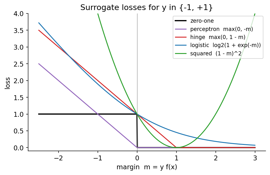
Which surrogates lead to the Bayes-optimal classifier when there is enough data? Bartlett, Jordan and McAuliffe [12] answered this precisely: a convex surrogate is classification-calibrated (minimizing its expected value yields the Bayes decision , with ) if and only if it is differentiable at with . Hinge, logistic, squared and exponential losses all qualify; the perceptron loss does not. They also relate the excess surrogate risk to the excess classification risk. Rosasco et al. [13] compared the convergence rates implied by different convex losses and concluded that, for classification, the hinge loss converges about as fast as the logistic loss and much faster than the square loss. The losses still differ in what they estimate: minimizing the expected logistic loss pointwise gives , so its scores are log-odds (probabilities after a sigmoid), whereas the pointwise minimizer of the expected hinge loss is , which carries no probability information. That is why SVM scores need separate calibration.
Code: compare linear classifiers on digits
The built-in digits dataset (8×8 images, 10 classes) requires no download. This is a single reproducible hold-out demonstration, not a benchmark ranking. Every scaler is fitted inside a pipeline, on training data only.
Code · Python · 25 lines
from sklearn.datasets import load_digits
from sklearn.discriminant_analysis import LinearDiscriminantAnalysis
from sklearn.linear_model import LogisticRegression, Perceptron, RidgeClassifier
from sklearn.metrics import accuracy_score
from sklearn.model_selection import train_test_split
from sklearn.pipeline import make_pipeline
from sklearn.preprocessing import StandardScaler
from sklearn.svm import LinearSVC

X, y = load_digits(return_X_y=True)
Xtr, Xte, ytr, yte = train_test_split(
    X, y, test_size=0.25, stratify=y, random_state=7)
models = {
    "least squares (ridge)": make_pipeline(StandardScaler(), RidgeClassifier(alpha=1.0)),
    "perceptron": make_pipeline(StandardScaler(),
                                Perceptron(max_iter=1500, random_state=7)),
    "logistic": make_pipeline(StandardScaler(),
                              LogisticRegression(C=1, max_iter=1500)),
    "linear SVM": make_pipeline(StandardScaler(),
                                LinearSVC(C=0.1, max_iter=20000, random_state=7)),
    "Gaussian LDA": LinearDiscriminantAnalysis(solver="lsqr", shrinkage="auto"),
}
for name, model in models.items():
    model.fit(Xtr, ytr)
    print(f"{name:22s} test accuracy: {accuracy_score(yte, model.predict(Xte)):.4f}")
On this split, logistic regression reaches , the linear SVM , the perceptron , and ridge-regularized least squares and shrinkage LDA each. All five are linear machines on the same 64 pixels; the differences come from the losses and regularization alone. Changing regularization after seeing these test results would turn this test set into a validation set. A real model-selection study needs a separate validation split or cross-validation inside the training partition (PR 09).
Modern view
Linear classifiers have not been replaced by deep learning; they have moved to the top of it. Three lines of recent work explain why they still matter, and the classic survey literature remains useful for the methods themselves.
Surveys and solvers. Burges’s tutorial [11] remains the most readable derivation of SVMs, from VC-dimension motivation through the dual and kernels. Cervantes et al. [17] survey SVM classification as of 2020: variants, applications, and challenges such as training cost on large datasets, class imbalance and model selection. On the computational side, LIBLINEAR [14] made linear SVMs and logistic regression with millions of sparse features routine, LIBSVM [16] is the reference kernel-SVM implementation behind scikit-learn’s SVC, and Pegasos [15] showed that stochastic sub-gradient descent on the SVM primal reaches a given accuracy with a run time that, for linear kernels, does not depend directly on the training-set size, the same idea as training neural networks with SGD.
Linear probes as the yardstick of representations. Alain and Bengio [21] proposed training independent linear classifiers (“probes”) on every layer of a network, and observed that linear separability increases monotonically with depth. Kornblith, Shlens and Le [22] compared 16 networks on 12 datasets and found that, with features used as fixed extractors under a logistic-regression classifier, ImageNet accuracy and transfer accuracy are strongly correlated, though some regularizers that slightly improve ImageNet accuracy produce much worse penultimate-layer features. CLIP [23] compares its zero-shot classifier with logistic-regression probes on frozen features, and DINOv2 [24] evaluates its self-supervised features largely with linear classifiers on frozen backbones. Kumar et al. [25] showed that full fine-tuning can distort good pretrained features and underperform a linear probe out of distribution, and proposed fitting a linear probe first and then fine-tuning (LP-FT). In other words: a well-regularized logistic regression on top of a frozen foundation model is a strong baseline, and often the right first experiment.
Implicit bias: logistic regression secretly finds the SVM. Soudry et al. [19] proved that gradient descent on unregularized logistic (or cross-entropy) loss over linearly separable data converges in direction to the hard-margin SVM solution, extending the result to other losses with exponential tails, to multiclass problems and to a restricted deep-network setting. Convergence is only logarithmic, which helps explain why continuing to train after zero training error can keep improving the margin. The gradient-descent code above shows the effect in two dimensions.
Neural collapse: Fisher’s picture at the end of training. Papyan, Han and Donoho [20] observed, across three architectures and seven datasets, that in the terminal phase of training (after zero training error) the last-layer features of each class collapse to their class mean, the class means arrange themselves into a maximally separated, symmetric configuration (a simplex equiangular tight frame), the classifier weights align with the class means, and the decision rule becomes the nearest class mean. In this chapter’s language, the within-class scatter shrinks towards zero, Fisher’s criterion grows without bound, and the network’s last layer becomes the minimum-distance classifier of PR 01.
Open problems. When should one trust a linear probe as a measure of representation quality, given that probe results depend on regularization and data size? How do implicit-bias results extend to realistic, non-separable, data-augmented training? And when do probabilities from linear heads stay calibrated under distribution shift? These questions link the oldest classifier in this track to current research.
Key takeaways
- A linear discriminant is a hyperplane with normal ; is the signed distance. Use one discriminant per class (a linear machine) for multiclass problems.
- Least squares and ridge have closed forms and a Bayesian MAP interpretation, but least squares is a poor classifier: it punishes points that are “too correct” and can mask classes.
- Fisher’s direction maximizes between-class over within-class spread; it equals the Gaussian LDA direction, which adds a threshold from means and priors.
- The perceptron converges in at most updates on separable data, but stops at an arbitrary separator and cycles on overlapping data.
- Logistic regression fits the log-odds by convex cross-entropy minimization (Newton/IRLS); without regularization its weights diverge on separable data, in the direction of the max-margin solution.
- The hard-margin SVM maximizes the margin ; its dual shows that only support vectors matter and that data enter only through inner products, which opens the door to kernels (PR 04). The soft margin is ridge-regularized hinge loss.
- All these methods are one linear score with different surrogate losses; hinge, logistic and squared losses are classification-calibrated, but only the logistic loss estimates probabilities.
Exercises
- Linear in the parameters. Show that fitting by least squares is a linear regression problem, and describe the decision regions in if the same features are used for a two-class linear classifier.
Hint
Build rows of a design matrix; the model is linear in . A quadratic in changes sign at most twice, so the region for one class can be an interval and the other class its complement (two half-lines).
- Units and ridge. Two features measure the same distance, one in metres and one in millimetres. Explain what ridge regression does without feature scaling, and why standardizing fixes it.
Hint
The millimetre coefficient can be 1,000 times smaller while describing the same effect, so it is penalized far less; ridge will load almost all weight onto the millimetre feature. After standardization both coordinates are penalized on the same scale.
- Fisher by hand. Two classes have means , and within-class scatter . Compute Fisher’s direction and compare it with the mean difference. When would the two directions coincide?
Hint
, so , rotated away from the mean difference because the classes are stretched along . The directions coincide exactly when is an eigenvector of , e.g. for .
- A perceptron that never stops. Construct a one-dimensional dataset on which the perceptron updates forever, and explain which assumption of the convergence theorem fails.
Hint
Put two points at the same coordinate with opposite labels (or any overlapping classes). No with exists, so the bound does not apply; each update that fixes one point breaks the other.
- SVM by hand. Find the hard-margin SVM for the two points with and with . Give , , the dual variables and the margin width, and check the KKT conditions.
Hint
By symmetry and . The constraint gives , so and the width is , the distance between the points. From and , . Both points are support vectors.
- Logistic versus hinge. Using the digits pipeline, fit
LogisticRegressionandLinearSVCfor several values ofCwith 5-fold cross-validation on the training set only. Compare their best validation accuracies, then compare their scores: which one gives meaningful probabilities, and how would you obtain probabilities from the other?
Hint
Accuracies are typically close, as the loss analysis predicts. Only logistic regression’s predict_proba estimates posteriors; for the SVM, fit a calibration map (Platt scaling or isotonic regression, e.g. CalibratedClassifierCV) on held-out data.
References
- R. O. Duda, P. E. Hart and D. G. Stork, Pattern Classification, 2nd ed., Wiley, 2001 (Ch. 5, linear discriminant functions). publisher page
- C. M. Bishop, Pattern Recognition and Machine Learning, Springer, 2006 (Sections 3.1–3.3, 4.1–4.3 and 7.1). official page and free PDF
- S. Theodoridis and K. Koutroumbas, Pattern Recognition, 4th ed., Academic Press, 2008 (Ch. 3, linear classifiers). publisher page
- T. Hastie, R. Tibshirani and J. Friedman, The Elements of Statistical Learning, 2nd ed., Springer, 2009 (Ch. 3–4 and 12). official page
- R. A. Fisher, “The use of multiple measurements in taxonomic problems,” Annals of Eugenics, vol. 7, no. 2, pp. 179–188, 1936. doi
- F. Rosenblatt, “The perceptron: a probabilistic model for information storage and organization in the brain,” Psychological Review, vol. 65, no. 6, pp. 386–408, 1958. doi
- D. R. Cox, “The regression analysis of binary sequences,” Journal of the Royal Statistical Society, Series B, vol. 20, no. 2, pp. 215–232, 1958. doi
- A. E. Hoerl and R. W. Kennard, “Ridge regression: biased estimation for nonorthogonal problems,” Technometrics, vol. 12, no. 1, pp. 55–67, 1970. doi
- B. E. Boser, I. M. Guyon and V. N. Vapnik, “A training algorithm for optimal margin classifiers,” in Proc. 5th Annual Workshop on Computational Learning Theory (COLT), pp. 144–152, 1992. doi
- C. Cortes and V. Vapnik, “Support-vector networks,” Machine Learning, vol. 20, no. 3, pp. 273–297, 1995. doi
- C. J. C. Burges, “A tutorial on support vector machines for pattern recognition,” Data Mining and Knowledge Discovery, vol. 2, no. 2, pp. 121–167, 1998. doi
- P. L. Bartlett, M. I. Jordan and J. D. McAuliffe, “Convexity, classification, and risk bounds,” Journal of the American Statistical Association, vol. 101, no. 473, pp. 138–156, 2006. doi
- L. Rosasco, E. De Vito, A. Caponnetto, M. Piana and A. Verri, “Are loss functions all the same?,” Neural Computation, vol. 16, no. 5, pp. 1063–1076, 2004. doi
- R.-E. Fan, K.-W. Chang, C.-J. Hsieh, X.-R. Wang and C.-J. Lin, “LIBLINEAR: a library for large linear classification,” Journal of Machine Learning Research, vol. 9, pp. 1871–1874, 2008. paper
- S. Shalev-Shwartz, Y. Singer, N. Srebro and A. Cotter, “Pegasos: primal estimated sub-gradient solver for SVM,” Mathematical Programming, vol. 127, no. 1, pp. 3–30, 2011. doi
- C.-C. Chang and C.-J. Lin, “LIBSVM: a library for support vector machines,” ACM Transactions on Intelligent Systems and Technology, vol. 2, no. 3, article 27, 2011. doi
- J. Cervantes, F. Garcia-Lamont, L. Rodríguez-Mazahua and A. Lopez, “A comprehensive survey on support vector machine classification: applications, challenges and trends,” Neurocomputing, vol. 408, pp. 189–215, 2020. doi
- A. Y. Ng and M. I. Jordan, “On discriminative vs. generative classifiers: a comparison of logistic regression and naive Bayes,” in Advances in Neural Information Processing Systems (NIPS), 2001. paper
- D. Soudry, E. Hoffer, M. S. Nacson, S. Gunasekar and N. Srebro, “The implicit bias of gradient descent on separable data,” Journal of Machine Learning Research, vol. 19, no. 70, pp. 1–57, 2018. paper
- V. Papyan, X. Y. Han and D. L. Donoho, “Prevalence of neural collapse during the terminal phase of deep learning training,” Proceedings of the National Academy of Sciences, vol. 117, no. 40, pp. 24652–24663, 2020. doi
- G. Alain and Y. Bengio, “Understanding intermediate layers using linear classifier probes,” arXiv:1610.01644, 2016. arXiv
- S. Kornblith, J. Shlens and Q. V. Le, “Do better ImageNet models transfer better?,” in Proc. IEEE/CVF Conference on Computer Vision and Pattern Recognition (CVPR), 2019. paper
- A. Radford et al., “Learning transferable visual models from natural language supervision,” in Proc. International Conference on Machine Learning (ICML), PMLR 139, 2021. paper
- M. Oquab et al., “DINOv2: learning robust visual features without supervision,” Transactions on Machine Learning Research, 2024. arXiv
- A. Kumar, A. Raghunathan, R. Jones, T. Ma and P. Liang, “Fine-tuning can distort pretrained features and underperform out-of-distribution,” in Proc. International Conference on Learning Representations (ICLR), 2022. arXiv
Check your understanding
This tutorial has 6 exercises. Can you solve them without opening the hints?
Go to the exercises ↑Next PR 04 · Neighbors, Kernels and Nonlinear Classifiers · 28 min