PR 08 · Approximate Inference and Bayesian Model Complexity
Needs: PR 07 · Clustering, Mixtures and EM
Navigate: this page and this track: Navigate: this page and this track
On this page
- What you’ll learn1 min
- The big picture1 min
- Why exact inference is hard2 min
- Monte Carlo: integrals as averages1 min
- Importance sampling2 min
- Markov chain Monte Carlo6 min
- Variational inference5 min
- Laplace approximation and expectation propagation2 min
- Evidence and complexity: Bayesian Occam’s razor1 min
- From the ELBO to VAEs and diffusion models1 min
- Choosing a method1 min
- Modern view2 min
- Key takeaways1 min
- Exercises3 min
- References
Pattern Recognition
Explore this chapter 1 interactive experiment
Move and widen a Gaussian approximation to a two-mode target; compare penalties for missing mass and filling the valley.
What you’ll learn
- Why Bayesian posteriors are easy to evaluate up to a constant but hard to integrate, and why grids fail beyond a handful of dimensions.
- How plain Monte Carlo, rejection sampling and importance sampling turn integrals into averages, and how to tell when their weights have collapsed.
- How Markov chain Monte Carlo works: detailed balance, Metropolis–Hastings (including the asymmetric-proposal correction), Gibbs sampling, Hamiltonian Monte Carlo, and the diagnostics (, effective sample size) that keep you honest.
- How variational inference turns integration into optimization: the evidence lower bound (ELBO) derived two ways, mean-field coordinate ascent, reverse versus forward KL, and stochastic gradients with the reparameterization trick.
- Where Laplace approximation and expectation propagation fit, how model evidence penalizes complexity, and how the same ideas power VAEs and diffusion models.
The big picture
Earlier chapters fitted one “best” parameter setting: maximum likelihood, MAP, or EM for mixtures. A Bayesian recognizer asks a bigger question. After seeing the data, how plausible is every parameter setting, and what do they predict on average? Answering it requires integrals over all unknowns. For almost every useful model those integrals have no closed form. This chapter is about the two families of workarounds: draw samples that behave like the posterior, or fit a simpler distribution that sits close to it.
Why it matters for recognition: uncertainty tells a system when to abstain (see PR 01), integrated evidence compares models without a held-out set, and the machinery of this chapter, especially the ELBO and Langevin-style sampling, is exactly what modern generative models use. We follow Bishop’s chapters on approximate inference and sampling [1]; Theodoridis and Koutroumbas supply the estimation and optimization background (Chapter 2 and Appendix C) rather than a one-to-one treatment of these methods [2].
Why exact inference is hard
Plain version. Bayes’ rule says the posterior is “prior times likelihood, divided by a normalizing number”. The top is usually easy to compute for any single guess. The bottom is a sum over every possible guess, and that is where the trouble starts.
Precise version. Collect all unknowns, latent variables and parameters, into , and write for the observed data. Then
where is the joint density (likelihood times prior) and is the evidence or marginal likelihood. Almost everything we want is an expectation under the posterior:
for example the posterior mean (), a predictive probability () or the probability that a parameter is positive (). We write for the unnormalized posterior: it is cheap to evaluate pointwise, but its normalizer is unknown.
Three things make the integral hard:
- Dimension. A grid with points per axis needs evaluations in dimensions. For and that is about , far beyond any computer.
- Concentration. With a lot of data the posterior occupies a tiny region of a huge space. Random guesses almost never land in it.
- Discrete structure. For a mixture with components and points, the latent assignments have configurations; summing over them exactly is hopeless even when each term is simple.
MAP estimation sidesteps all of this by maximizing , but a maximum is not an integral. The highest point of the posterior can sit in a narrow spike that carries little mass, and a single point carries no information about spread. EM, from PR 07, sits in between: it integrates over latent assignments in its E step (which is tractable for Gaussian mixtures) but still returns a point estimate of the parameters.
A worked example: Bayesian logistic regression
Take a two-class problem with inputs (a bias feature and one measurement), labels , weights and the model
The log joint is plus a constant. The Gaussian prior is not conjugate to the logistic likelihood, so the posterior is not Gaussian and its normalizer has no formula. With only two weights we can still brute-force it on a grid, which gives us a ground truth to compare every approximation against.
Code · Python · 25 lines
import numpy as np

rng = np.random.default_rng(0)
n = 40
X = np.c_[np.ones(n), rng.normal(size=n)]
w_true = np.array([-0.5, 1.5])
y = rng.random(n) < 1 / (1 + np.exp(-X @ w_true))

def log_joint(w):                       # log p(y | X, w) + log p(w), w ~ N(0, 2^2 I)
    s = X @ w
    return np.sum(y * s - np.logaddexp(0, s)) - 0.5 * np.sum(w**2) / 4.0

# Brute-force normalization on a grid: fine in 2-D, hopeless in 50-D.
g = np.linspace(-4, 4, 201)
W0, W1 = np.meshgrid(g, g, indexing="ij")
logp = np.array([[log_joint(np.array([a, b])) for b in g] for a in g])
cell = (g[1] - g[0])**2
log_evidence = np.log(np.sum(np.exp(logp - logp.max())) * cell) + logp.max()
post = np.exp(logp - log_evidence)
mean = np.array([np.sum(W0 * post), np.sum(W1 * post)]) * cell
sd = np.sqrt(np.array([np.sum((W0 - mean[0])**2 * post),
                       np.sum((W1 - mean[1])**2 * post)]) * cell)
print("log evidence:", round(log_evidence, 3))
print("posterior mean:", mean.round(3), " sd:", sd.round(3))
print("grid points for 201 per axis in 50-D:", f"{201.0**50:.2e}")
It prints a log evidence of , a posterior mean of and standard deviations of . Note the subtraction of logp.max() before exponentiating: log densities of real data are large negative numbers, and working in log space (the “log-sum-exp” trick) is the first habit of every practitioner. We will reuse this model to judge the Laplace and variational approximations later in the chapter.
Monte Carlo: integrals as averages
Plain version. If you can draw random examples from a distribution, the average of a quantity over those examples estimates its expected value. More draws give a better estimate, and the error shrinks in a predictable way that does not depend on the dimension.
Precise version. Given independent draws , the Monte Carlo estimator of is
Here is the number of samples and is the variance of under . Assuming is finite, the estimator is unbiased; the displayed variance and the standard-error statement additionally require finite : to halve the error you need four times as many samples. The striking part is that does not appear. The rate exponent is dimension independent, but the variance of and the cost of obtaining each draw can grow with dimension. Heavy-tailed quantities with infinite variance do not have this standard-error guarantee.
The catch is the assumption “draws from ”. For a posterior we usually cannot sample directly. The rest of the sampling half of this chapter is about manufacturing such draws, or correcting for draws from the wrong distribution.
Rejection sampling
Suppose we can sample from a simple proposal and know a constant with for all . Draw and , and keep if . The kept points are exact draws from , because the accepted region under the envelope has exactly the shape of . The acceptance probability is , where . In high dimensions a usable envelope must be enormous compared with the target, so almost everything is rejected. Rejection sampling is a building block for one-dimensional conditionals (for example inside Gibbs samplers), not a general posterior engine [1].
Importance sampling
Plain version. Draw from a convenient distribution, then correct each draw with a weight that says how much more (or less) likely it is under the distribution you actually care about. Works well when the convenient distribution covers the important region; fails quietly when it does not.
Precise version. For any with wherever ,
The ratio is the importance weight. When only is available, the unknown cancels if we normalize the weights:
For self-normalization and evidence estimation, strengthen the support condition to wherever , including regions where : the denominator must account for the whole target mass. Otherwise normalization estimates a truncated target rather than the intended posterior.
This self-normalized estimator is generally biased for finite but consistent as . As a by-product, is an unbiased estimate of the evidence , which is how importance sampling is used for model comparison.
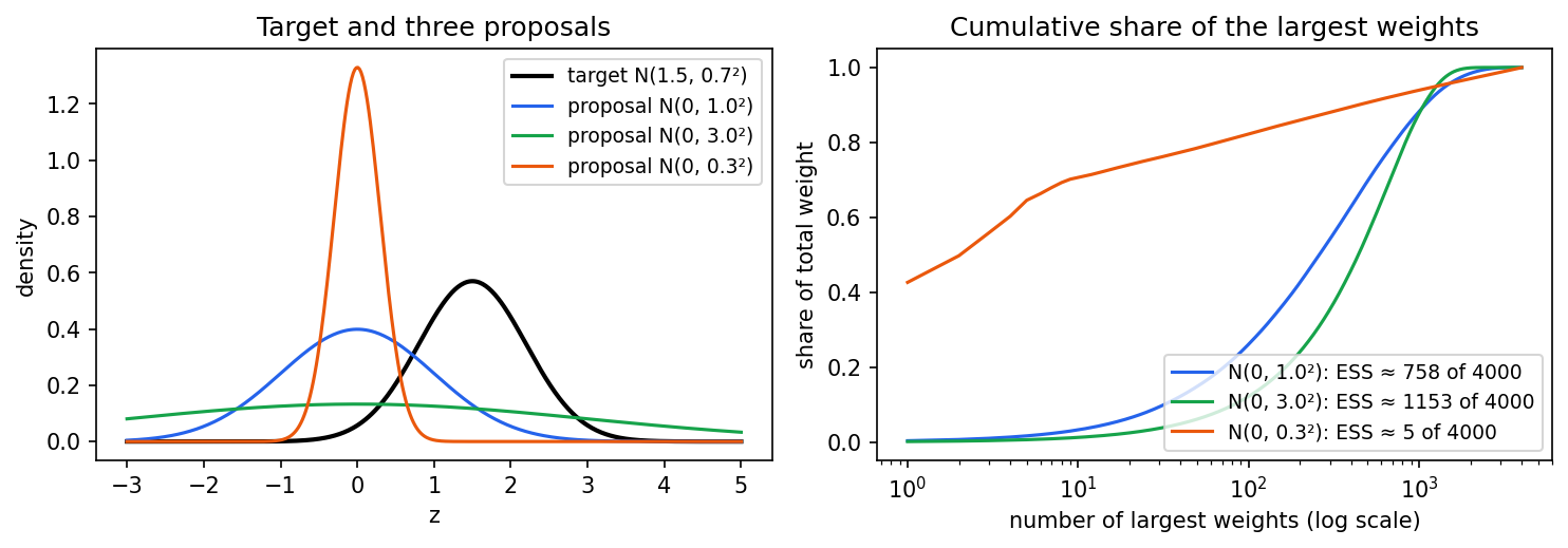
The quality of the estimate depends on how uneven the weights are. A widely used summary is the effective sample size of the weights,
which equals when all weights are equal and when one weight takes everything. Two failure modes matter:
- Proposal too narrow or misplaced. Regions where has mass but is tiny produce rare, gigantic weights. The estimate is dominated by a handful of draws and its variance can even be infinite.
- Light tails. The ratio must stay bounded in the tails. A rule of thumb is to make heavier-tailed than (a Student- instead of a Gaussian, or a wider Gaussian).
Code · Python · 28 lines
import numpy as np
from scipy.stats import norm

rng = np.random.default_rng(1)
N = 10_000
exact = norm.sf(3.0)                      # P(X > 3) for X ~ N(0, 1)

# Plain Monte Carlo: most samples never reach the tail.
x = rng.normal(0, 1, N)
plain = np.mean(x > 3)

# Importance sampling with a proposal centered on the tail, q = N(3, 1).
z = rng.normal(3, 1, N)
w = norm.pdf(z) / norm.pdf(z, loc=3)      # p(z) / q(z)
is_est = np.mean(w * (z > 3))
print(f"exact {exact:.6f}  plain MC {plain:.6f}  importance {is_est:.6f}")

# Self-normalized IS for an unnormalized target, with effective sample size.
def log_p_tilde(t):                       # N(1.5, 0.7^2) without its constant
    return -0.5 * ((t - 1.5) / 0.7) ** 2

for scale in [1.0, 3.0, 0.3]:
    t = rng.normal(0, scale, N)
    log_w = log_p_tilde(t) - norm.logpdf(t, scale=scale)
    wn = np.exp(log_w - log_w.max())
    wn /= wn.sum()
    ess = 1.0 / np.sum(wn**2)
    print(f"proposal N(0,{scale}^2): mean {np.sum(wn * t):.3f}  ESS {ess:7.1f} of {N}")
The rare-event estimate shows why importance sampling exists: the exact tail probability is ; plain Monte Carlo with 10,000 draws gives (only 19 draws landed in the tail), while the shifted proposal gives . In the second part the target mean is . The wide proposals give and with ESS of about 1,870 and 2,830. The narrow proposal gives with an ESS of 13, a confident-looking but wrong answer. A tiny ESS is the alarm bell.
Importance sampling stays important even when it is not the main engine: it re-weights samples from an old model to a new one, it estimates evidence, and it powers sequential Monte Carlo (particle filters), where weights are refreshed and resampled step by step as data arrive.
Markov chain Monte Carlo
Plain version. Instead of drawing independent samples, take a random walk whose rules are designed so that, in the long run, the fraction of time spent in each region equals the posterior probability of that region. Then time averages along the walk estimate posterior expectations. Successive steps are correlated, so a long walk is worth fewer independent draws than its length suggests.
Precise version. A Markov chain with transition kernel has as a stationary (invariant) distribution if
A simple sufficient condition is detailed balance (reversibility):
Integrating both sides over gives stationarity. If the chain can also reach every region (irreducibility) and does not cycle (aperiodicity), the distribution of the state converges to from any starting point, and the ergodic average converges to . Importantly, detailed balance involves only ratios , so the unknown normalizer cancels.
Metropolis–Hastings
The Metropolis algorithm [3], generalized by Hastings [4], builds such a kernel from any proposal :
- From the current state , propose .
- Accept with probability
- If accepted, move to ; otherwise stay at and record again.
Here is the density of proposing the reverse move. The factor is the Hastings correction: it cancels any bias the proposal has toward certain directions. For a symmetric proposal such as a Gaussian random walk, and the rule reduces to Metropolis’s original .
To see why it works, take and suppose . Then , and in the reverse direction the acceptance is 1, so . Both sides match: detailed balance holds.
Forgetting step 3 (only recording accepted states) is a classic bug: it over-represents regions the chain moves through easily and biases every estimate.
A Gaussian target with known moments lets us check a random-walk chain. The assertions are deliberately loose: a numerical sanity check, not a convergence proof.
Code · Python · 20 lines
import numpy as np

rng = np.random.default_rng(12)
def log_target(x):
    return -0.5 * ((x - 1.5) / 0.7)**2
x, accepted = -3.0, 0
samples = []
for step in range(18000):
    proposal = x + rng.normal(0, 0.8)
    if np.log(rng.random()) < min(0.0, log_target(proposal) - log_target(x)):
        x = proposal
        accepted += 1
    if step >= 2000:                      # discard warm-up, keep repeats
        samples.append(x)
samples = np.asarray(samples)
rho1 = np.corrcoef(samples[:-1], samples[1:])[0, 1]
print("mean, std:", samples.mean(), samples.std())
print("acceptance:", accepted / 18000, "lag-one correlation:", rho1)
assert abs(samples.mean() - 1.5) < 0.12
assert abs(samples.std() - 0.7) < 0.12
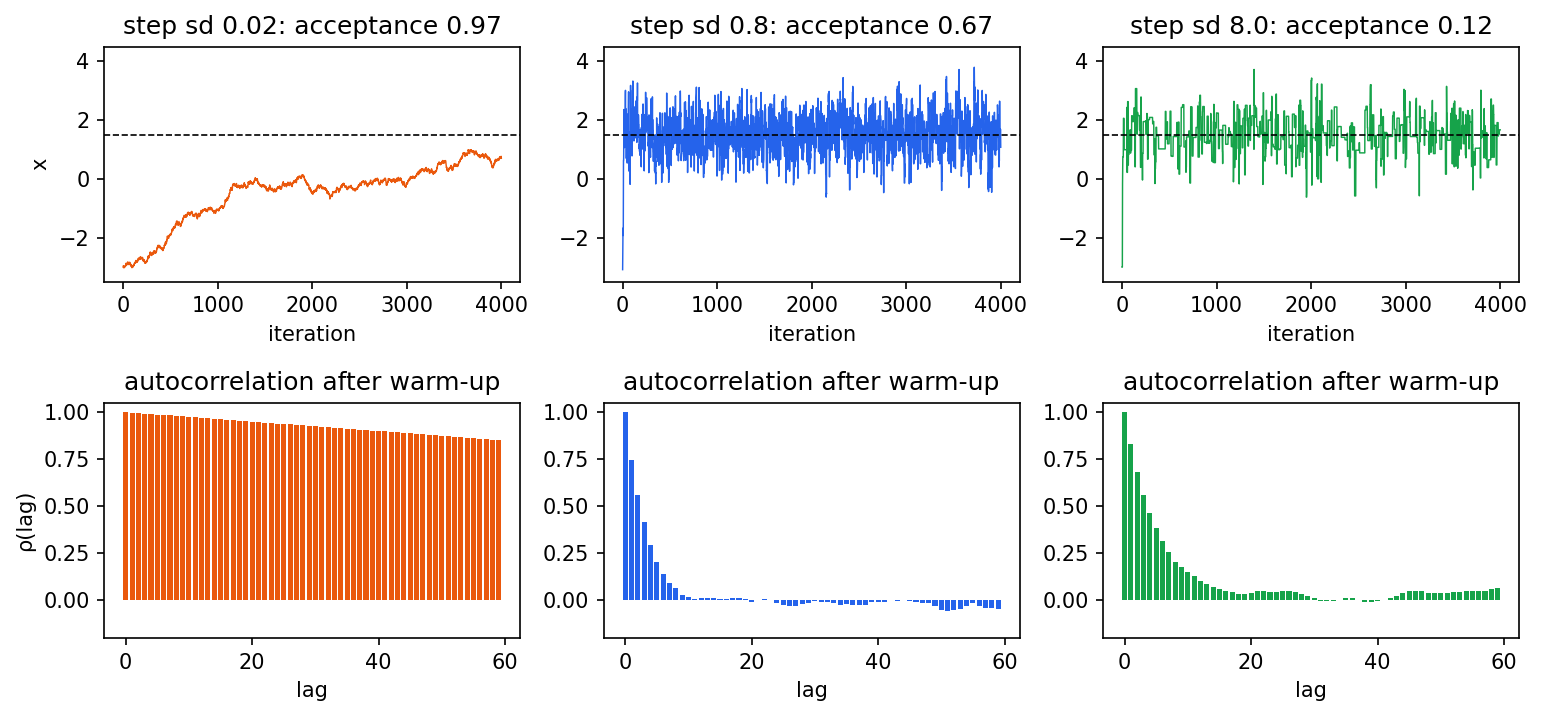
The chain recovers mean and standard deviation , with acceptance and lag-one correlation . The step size is the main tuning knob, and acceptance alone does not tell you whether it is good. Tiny steps are almost always accepted but crawl; huge steps are mostly rejected and the chain sits still. Both produce strongly correlated samples.
Gibbs sampling
Plain version. Update one variable (or block) at a time by drawing it from its distribution given all the others. If those conditional distributions are easy, as they often are in conjugate models, every move is accepted.
Precise version. Gibbs sampling, introduced for image restoration with Markov random fields by Geman and Geman [5], cycles through blocks and draws
where denotes all blocks except . It is a special case of Metropolis–Hastings with proposal and ; plugging into the acceptance ratio gives exactly 1 [1]. In a Gaussian mixture, for example, one alternates between sampling each point’s component label from its responsibilities and sampling the component parameters from their conjugate posteriors: a stochastic cousin of EM.
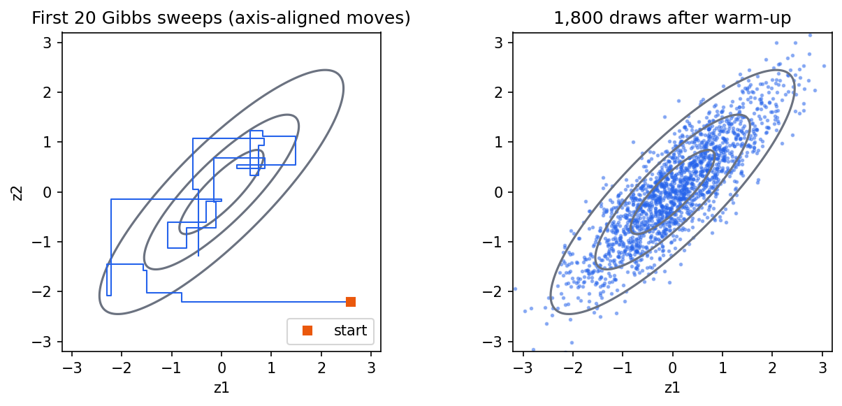
For a zero-mean bivariate Gaussian with unit variances and correlation , the conditionals are and symmetrically for . The code below runs four chains from dispersed corners and computes the split- convergence diagnostic described in the next subsection.
Code · Python · 31 lines
import numpy as np

rng = np.random.default_rng(3)
rho = 0.85                     # target: zero-mean bivariate Gaussian, unit variances
sd = np.sqrt(1 - rho**2)       # conditional standard deviation

def gibbs(n_steps, start):
    z = np.array(start, dtype=float)
    out = np.empty((n_steps, 2))
    for t in range(n_steps):
        z[0] = rng.normal(rho * z[1], sd)   # z1 | z2 ~ N(rho z2, 1 - rho^2)
        z[1] = rng.normal(rho * z[0], sd)   # z2 | z1 ~ N(rho z1, 1 - rho^2)
        out[t] = z
    return out

def split_rhat(chains):        # chains: (m, n) draws of one scalar quantity
    m, n = chains.shape
    halves = chains[:, : n // 2 * 2].reshape(2 * m, n // 2)
    W = halves.var(axis=1, ddof=1).mean()          # within-chain variance
    B = (n // 2) * halves.mean(axis=1).var(ddof=1) # between-chain variance
    var_plus = (n // 2 - 1) / (n // 2) * W + B / (n // 2)
    return np.sqrt(var_plus / W)

starts = [(-4, -4), (4, 4), (-4, 4), (4, -4)]
chains = np.stack([gibbs(3000, s)[500:] for s in starts])   # drop warm-up
draws = chains.reshape(-1, 2)
print("sample correlation:", np.corrcoef(draws.T)[0, 1].round(3))
print("sample variances:", draws.var(axis=0).round(3))
lag1 = np.mean([np.corrcoef(c[:-1, 0], c[1:, 0])[0, 1] for c in chains])
print("lag-1 autocorrelation of z1:", lag1.round(3), " (theory rho^2 =", rho**2, ")")
print("split R-hat for z1:", split_rhat(chains[:, :, 0]).round(4))
Output: sample correlation , variances near , lag-one autocorrelation (theory ) and split- . The autocorrelation is the price of axis-aligned moves: when the target is a long diagonal ridge, each coordinate can only move a short distance before hitting the walls. As the chain slows to a crawl. Reparameterizing (rotating or whitening the variables) or updating correlated variables together as a block fixes this.
Hamiltonian Monte Carlo
Plain version. Random walks waste effort going back and forth. Hamiltonian Monte Carlo (HMC) uses the gradient of the log posterior to glide along the distribution like a frictionless puck on a curved surface, making long, informed moves that are still accepted with high probability.
Precise version. Define potential energy , add an auxiliary momentum with mass matrix , and form the Hamiltonian
Hamiltonian dynamics conserve and preserve volume. In practice we simulate them with leapfrog steps of size :
The leapfrog integrator is reversible and volume-preserving but not exactly energy-conserving, so the endpoint is accepted with probability , a Metropolis step on the joint space [6]. Because the trajectory follows the geometry of the target, HMC can traverse a correlated ridge that would trap Gibbs or a random walk. Its tuning parameters, and , are delicate; the No-U-Turn Sampler (NUTS) chooses the trajectory length automatically by stopping when the path starts to double back, and adapts during warm-up [7]. Betancourt’s conceptual introduction explains why HMC scales to high dimensions in terms of the typical set, the thin shell where posterior mass actually lives [8]. HMC needs differentiable, continuous targets; discrete latent variables must be summed out or handled by other moves.
A close relative is the Langevin update
which is one leapfrog step with freshly drawn momentum. Without an accept/reject step it is only approximately correct for finite ; with the Metropolis correction it becomes the Metropolis-adjusted Langevin algorithm. Keep this update in mind: it reappears in diffusion models.
Diagnostics: is the chain telling the truth?
No finite run proves convergence. Diagnostics can only reveal problems. Standard practice:
- Run several chains from dispersed starting points and discard an initial warm-up portion of each.
- Compare chains with . With chains (split in halves) of length , let be the average within-chain variance and the variance of the chain means. Then
If all chains explore the same distribution, ; values noticeably above 1 mean the chains disagree. Vehtari et al. showed that the classic version misses heavy tails and differences in scale, and proposed a rank-normalized, folded split- together with bulk and tail effective sample sizes; this is the version current software reports [9].
- Report effective sample size. For a stationary chain with lag- autocorrelation of the quantity of interest,
where the sum is truncated once estimated autocorrelations become noisy. The Monte Carlo standard error is roughly , not . For the Gibbs chain above, , so : 10,000 stored draws are worth about 1,600 independent ones.
- Look at traces and, for gradient-based samplers, at divergence warnings, which flag regions of high curvature the integrator cannot follow.
Different quantities mix at different speeds: a mean can look fine while a tail quantile has not converged. And a perfectly mixing chain still only describes the posterior of the model you wrote down; it says nothing about whether that model is right.
Variational inference
Plain version. Pick a family of simple distributions (for example, independent Gaussians), and search within it for the member closest to the posterior. Integration becomes optimization, which is fast and scales to huge datasets, at the cost of a bias you cannot remove by running longer.
Precise version. Choose a family of tractable densities , indexed by variational parameters . Variational inference (VI) [10] solves
We cannot evaluate this KL directly because it contains the unknown . The trick is the ELBO.
The ELBO, derived two ways
Derivation 1: decomposition. Substitute into the KL:
Rearranging,
Because does not depend on , maximizing is exactly minimizing the KL. Because KL is nonnegative, : it is the evidence lower bound, ELBO.
Derivation 2: Jensen’s inequality. Multiply and divide by inside the evidence integral and use the concavity of :
The first equality assumes covers the support of . If it omits positive joint mass, the expectation integrates only over the support of ; it is no longer equal to the full evidence. The ELBO remains a lower bound via derivation 1 whenever the terms are well-defined. Under the coverage assumption, the gap in Jensen’s inequality is exactly that KL. A useful reading of the ELBO is : fit the data, but do not stray too far from the prior. EM is the special case where over latent variables is set to the exact posterior in the E step (making the bound tight) and the bound is then maximized over parameters in the M step [1].
Mean field and coordinate ascent (CAVI)
The most common family is mean field: , independent factors over blocks of . Holding all factors except fixed and maximizing the ELBO over gives
where averages over all other factors and the constant normalizes . (To derive it, write as a function of only; it equals plus a constant, where .) Cycling through is coordinate ascent variational inference (CAVI). Each update cannot decrease the ELBO, so CAVI converges, but only to a local optimum [11]. For conditionally conjugate models each stays in the same family as the prior and the updates are closed-form.
Worked example: a Gaussian with unknown mean and precision. Observations , prior , . The exact posterior is known (Normal–Gamma), so we can grade the approximation. With the mean-field update rule gives and with [1]
where is the sample mean and . The two factors depend on each other through and , so we iterate.
Code · Python · 28 lines
import numpy as np

# Data x_n ~ N(mu, 1/tau); prior mu | tau ~ N(mu0, 1/(lam0 tau)), tau ~ Gamma(a0, b0).
rng = np.random.default_rng(4)
x = rng.normal(2.0, 0.5, size=30)
N, xbar = len(x), x.mean()
mu0, lam0, a0, b0 = 0.0, 1.0, 1.0, 1.0

# Mean field q(mu, tau) = q(mu) q(tau) with q(mu) = N(mu_N, 1/lam_N), q(tau) = Gamma(a_N, b_N).
E_tau = a0 / b0
for it in range(50):
    mu_N = (lam0 * mu0 + N * xbar) / (lam0 + N)
    lam_N = (lam0 + N) * E_tau
    a_N = a0 + (N + 1) / 2
    E_mu, E_mu2 = mu_N, mu_N**2 + 1 / lam_N
    b_N = b0 + 0.5 * (np.sum(x**2) - 2 * E_mu * np.sum(x) + N * E_mu2
                      + lam0 * (E_mu2 - 2 * mu0 * E_mu + mu0**2))
    E_tau = a_N / b_N

# Exact posterior is Normal-Gamma: compare the marginal moments of mu.
lam_post = lam0 + N
mu_post = (lam0 * mu0 + N * xbar) / lam_post
a_post = a0 + N / 2
b_post = b0 + 0.5 * (np.sum((x - xbar) ** 2) + lam0 * N * (xbar - mu0) ** 2 / lam_post)
var_mu_exact = b_post / ((a_post - 1) * lam_post)       # Student-t marginal variance
print("E[mu]   VI %.4f  exact %.4f" % (mu_N, mu_post))
print("Var[mu] VI %.5f  exact %.5f" % (1 / lam_N, var_mu_exact))
print("E[tau]  VI %.3f   exact %.3f" % (a_N / b_N, a_post / b_post))
The means agree ( both) and so does (), but the variance of is under VI against exactly: about 6% too small. Under the exact posterior, and are dependent (the spread of scales with ) and its marginal is a heavier-tailed Student-; a factorized Gaussian cannot represent either property.
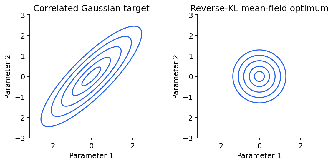
This underestimation is systematic. For a Gaussian target with precision matrix , the optimal mean-field factor has variance , the conditional variance, which is never larger than the marginal variance. Figure 4 shows the extreme case.
Which KL? Mode seeking versus mass covering
KL is not symmetric, and the direction changes the answer. Reverse KL, , used by standard VI, takes expectations under : it heavily penalizes putting -mass where is tiny, but does not mind if ignores some of . The result is mode seeking and under-dispersed. Forward KL, , takes expectations under : it heavily penalizes missing any region where has mass, so stretches to cover everything, which is mass covering and can put mass in the valleys between modes. Within an exponential family such as the Gaussians, minimizing forward KL is exactly moment matching: takes the mean and covariance of .
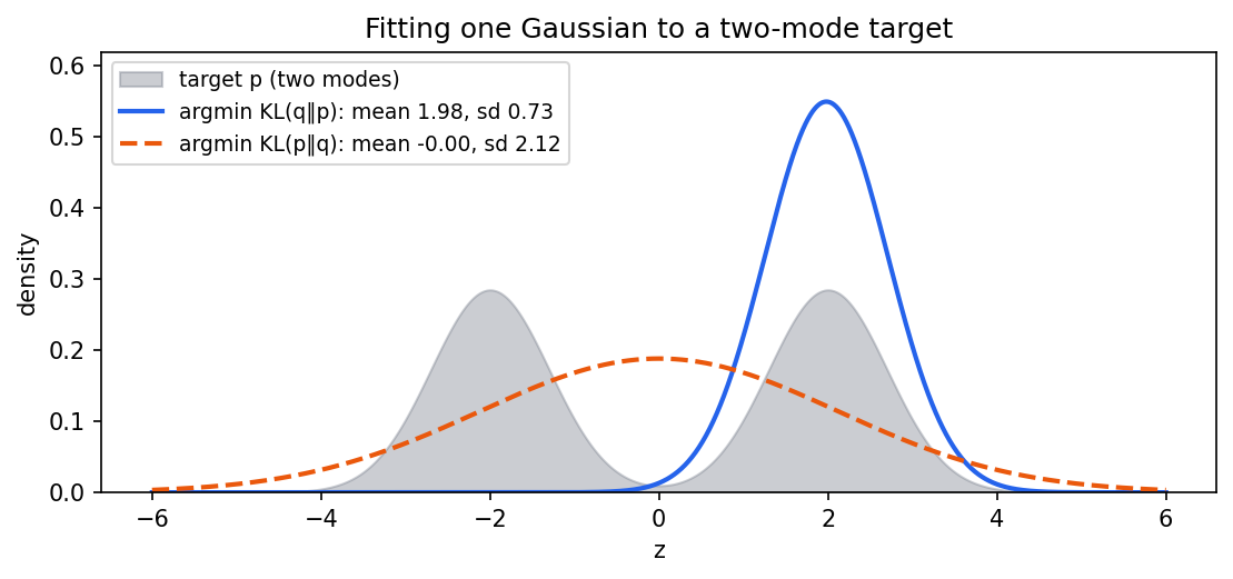
Neither direction is “right”. Reverse KL is tractable and gives sharp, usable answers but understates uncertainty. Forward KL is the objective behind expectation propagation and behind maximum-likelihood fitting of a model to data, and it is safer when missing a mode is costly.
Stochastic and black-box VI
CAVI needs conjugacy and passes over the whole dataset per update. Modern VI instead takes stochastic gradients of the ELBO, which works for almost any model and scales to large data by subsampling minibatches [11, 12]. There are two main gradient estimators for :
- Score-function (REINFORCE) estimator, used by black-box VI [13]:
It needs only evaluations of and works for discrete , but has high variance and needs control variates.
- Reparameterization (pathwise) estimator. Write with noise from a fixed distribution, for example with . Then
It requires differentiable and continuous but typically has much lower variance. This is the estimator the VAE made famous [15].
For a diagonal Gaussian with , , the entropy term is plus a constant, so its gradient with respect to is simply 1. Applied to the logistic-regression posterior:
Code · Python · 32 lines
import numpy as np

rng = np.random.default_rng(0)
n = 40
X = np.c_[np.ones(n), rng.normal(size=n)]
y = (rng.random(n) < 1 / (1 + np.exp(-X @ np.array([-0.5, 1.5])))).astype(float)
prior_var = 4.0

def grad_log_joint(W):                  # W: (S, 2) -> gradients (S, 2)
    p = 1 / (1 + np.exp(-W @ X.T))      # (S, n)
    return (y - p) @ X - W / prior_var

# Laplace: Newton's method to the MAP, then invert the Hessian.
w = np.zeros(2)
for _ in range(25):
    p = 1 / (1 + np.exp(-X @ w))
    H = X.T @ (X * (p * (1 - p))[:, None]) + np.eye(2) / prior_var
    w = w + np.linalg.solve(H, grad_log_joint(w[None])[0])
print("Laplace mean:", w.round(3), " sd:", np.sqrt(np.diag(np.linalg.inv(H))).round(3))

# Mean-field Gaussian VI with reparameterization: w = m + exp(s) * eps.
m, s = np.zeros(2), np.full(2, -1.0)
lr, S = 0.02, 64
for step in range(3000):
    eps = rng.normal(size=(S, 2))
    W = m + np.exp(s) * eps
    g = grad_log_joint(W)
    grad_m = g.mean(axis=0)                                # d ELBO / d m
    grad_s = (g * eps).mean(axis=0) * np.exp(s) + 1.0      # + entropy term
    m += lr * grad_m
    s += lr * grad_s
print("VI mean:     ", m.round(3), " sd:", np.exp(s).round(3))
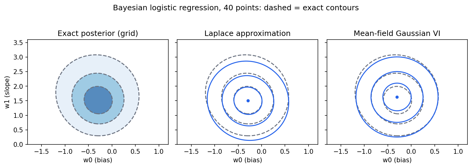
Compare with the grid truth, mean and sd . The code prints a Laplace mean of with sd , and a VI mean of with sd . VI recovers the posterior mean almost exactly, because it averages over the skewed posterior; Laplace reports the mode, which differs from the mean when the posterior is skewed. Both slightly understate the spread. With 40 data points the posterior is nearly Gaussian, so the differences are small; with fewer points or separable classes they grow quickly.
Laplace approximation and expectation propagation
Laplace: a Gaussian at the peak
Plain version. Find the highest point of the posterior and fit a Gaussian whose curvature matches the curvature there.
Precise version. Expand to second order around a mode , where the gradient is zero. With the Hessian of the negative log posterior,
where is the dimension of . The second formula is the Laplace evidence approximation; keeping only the terms that grow with gives the BIC criterion used for choosing the number of mixture components in PR 07 [1]. Laplace is cheap (one optimization and one Hessian) and becomes accurate as data accumulate, because posteriors of regular models become increasingly Gaussian. It fails for skewed posteriors, for modes on a boundary (such as a variance near zero), when the Hessian is singular, and for multi-modal posteriors, where it describes only one mode. Modern “Laplace for deep networks” methods apply it to the last layer or with structured Hessian approximations to obtain cheap uncertainty for trained neural networks.
Expectation propagation
Expectation propagation (EP) [14] targets posteriors that factor as , for example one factor per data point. It approximates each factor by a simple site from an exponential family, so , and refines sites one at a time:
- Remove site to form the cavity .
- Form the tilted distribution , the cavity times the exact factor.
- Set the new to the member of the family that matches the moments of , i.e. minimizes the forward KL .
- Update the site: .
Because each step uses forward KL locally, EP tends to cover mass and often gives better-calibrated variances than mean-field VI, for example in Gaussian-process classification. In exchange, it has no global objective that is guaranteed to improve, can fail to converge, and may produce invalid (negative-variance) sites that need damping [1, 14].
Evidence and complexity: Bayesian Occam’s razor
Plain version. A model that can explain anything spreads its prior bets thin, so it gets little credit for explaining the data you actually saw. A simpler model that bet on this kind of data gets more credit.
Precise version. The evidence of model integrates the likelihood against the prior,
A flexible model can reach a high peak likelihood, yet if most of its prior mass sits on parameters that fit badly, the integral is small. The Laplace formula makes this explicit: the evidence is the peak value times an “Occam factor” that compares posterior volume with prior volume. Two cautions follow. First, the evidence depends on the prior, even on aspects that barely affect the posterior, such as how wide a vague prior is. Second, it answers “which model would have predicted this data set?”, which is related to but not identical to “which model will predict new data best?”. Held-out validation (PR 09) answers the second. Comparing ELBOs across models is also delicate: each ELBO undershoots its evidence by a different, unknown KL gap.
From the ELBO to VAEs and diffusion models
The machinery in this chapter is the backbone of two families of deep generative models covered in the ML track.
VAEs are amortized variational inference. A variational autoencoder models images with a latent code , a prior , and a neural decoder . Instead of optimizing separate variational parameters for every image, an encoder network outputs them: . This is amortized inference: one network learns to perform inference for any input. The per-image objective is exactly the ELBO,
trained jointly over and with the reparameterization gradient [15, 16]. Its known weaknesses are the ones above: an amortization gap (the encoder’s answer is worse than per-image optimization), the under-dispersion of reverse KL, and a Gaussian decoder that blurs. See ML 07 for a full treatment and code.
Diffusion models are trained with an ELBO and sampled with Langevin-style dynamics. A denoising diffusion probabilistic model fixes a forward process that gradually adds Gaussian noise, , and learns a reverse process . The forward noisy states play the role of latent variables, with the forward process as a fixed variational posterior; the training objective is a variational bound on , and the popular noise-prediction loss is a reweighted form of that bound [17]. The score-based view [18] instead learns , the gradient of the log density of noisy data, and generates samples by integrating a reverse-time stochastic differential equation; its predictor–corrector samplers explicitly interleave Langevin MCMC steps that use in place of . The only change from the Langevin update earlier in this chapter is that the score is learned from data rather than computed from a formula. See ML 08.
Choosing a method
| Method | What it returns | Strengths | Main failure mode |
|---|---|---|---|
| Grid / quadrature | numerical approximation | low-dimensional reference after refinement checks | truncation/discretization error; cost grows rapidly with dimension |
| Importance sampling | weighted samples, evidence | simple, parallel, gives | weight collapse when misses |
| Random-walk MH | correlated samples | needs only | slow in high dimension; tuning |
| Gibbs | correlated samples | no tuning when conditionals are easy | slow on correlated variables |
| HMC / NUTS | correlated samples | scales to many continuous parameters | needs gradients; discrete variables; divergences |
| Mean-field VI | a distribution | fast, scalable, minibatch-friendly | under-dispersion; local optima |
| Laplace | Gaussian at the mode | cheap; evidence estimate | skew, boundaries, multiple modes |
| EP | Gaussian / exponential family | often good variances | may not converge |
A sensible workflow is to start with an optimizer (MAP or VI) for speed, check it against a careful sampler on a smaller version of the problem, and use simulation from known parameters to verify that the whole pipeline recovers what it should.
Modern view
Surveys worth reading. Blei, Kucukelbir and McAuliffe’s review for statisticians [11] is the standard entry point to VI: it derives the ELBO and CAVI, works through Gaussian mixtures, introduces stochastic VI, and is explicit that VI trades MCMC’s asymptotic exactness for speed, tending to underestimate posterior variance. Zhang, Bütepage, Kjellström and Mandt [12] organize the later literature into four axes: scalable VI (stochastic and distributed), generic VI for nonconjugate models (black-box and reparameterization gradients), accurate VI (alternative divergences beyond reverse KL, richer families) and amortized VI (inference networks, VAEs). Jordan, Ghahramani, Jaakkola and Saul [10] is the classic introduction to variational methods for graphical models and remains the clearest source for the convex-duality view. On the sampling side, Neal’s chapter [6] is the canonical derivation of HMC, Betancourt [8] gives the geometric picture of why it works in high dimensions, and Hoffman and Gelman [7] describe NUTS, the default sampler in modern probabilistic programming systems. Vehtari et al. [9] set the current standard for convergence diagnostics. Kingma and Welling’s monograph [16] surveys VAEs as amortized VI, and Yang et al. [19] survey diffusion models, including their variational and score-based formulations.
State of the art, 2023–2026. Three trends stand out.
- Machine learning inside Bayesian computation. Winter, Campbell, Lin, Srivastava and Dunson [20] review how normalizing flows, Bayesian coresets, distributed inference and variational methods are being used to speed up posterior computation, and where the guarantees are still weaker than for classical MCMC.
- Diffusion ideas used for sampling, not just generation. When only an unnormalized density is available (no data), one can still train a diffusion-style sampler. Denoising Diffusion Samplers [21] learn to reverse a noising process so that it ends at a target known only up to a constant, giving approximate samples and an estimate of the normalizing constant; they connect to optimal control and Schrödinger bridges and are a representative member of a growing family of learned samplers for Bayesian and physics problems.
- Workflows over single algorithms. Practice has moved toward probabilistic programming systems that run NUTS by default, report rank-normalized and bulk/tail ESS [9], and use VI or Laplace as fast first passes rather than final answers.
Open problems. Reliable uncertainty for very large models remains hard: full-batch MCMC is too expensive, and cheap approximations (mean-field VI, last-layer Laplace, ensembles) disagree. Multi-modal posteriors defeat both local VI and single chains. Evaluating the quality of an approximation without ground truth is still largely heuristic, and comparing models through ELBOs is confounded by unknown approximation gaps.
Key takeaways
- Posteriors are easy to evaluate up to a constant and hard to integrate; grids cost , so approximation is unavoidable beyond a few dimensions.
- Monte Carlo error falls as regardless of dimension, but only if you can draw from the right distribution. Importance sampling corrects for the wrong one, and the weight ESS tells you when the correction has collapsed.
- Metropolis–Hastings needs only ratios of and a Hastings correction for asymmetric proposals. Gibbs is MH with acceptance 1. HMC uses gradients to move far. Always record rejected states, run several chains, and check and ESS.
- VI maximizes the ELBO, which equals minimizing reverse KL to the posterior. It is fast and scalable, mode seeking, and tends to underestimate variance, especially under mean field.
- Laplace fits a Gaussian at the mode and gives a cheap evidence estimate (and BIC); EP matches moments locally and often gives better variances but may not converge.
- The evidence implements Occam’s razor but depends on priors and answers a different question from held-out prediction.
- VAEs are amortized VI with the reparameterization gradient; diffusion models are trained with a variational bound and sampled with Langevin-like dynamics driven by a learned score.
Exercises
- ELBO by hand. Starting from , derive . Then show that when the bound is tight, and explain how this makes EM a special case of maximizing the ELBO.
Hint
Substitute and pull out of the expectation because it does not depend on . With equal to the posterior, the KL is zero. EM’s E step sets to the posterior of the latent variables at the current parameters (tight bound); its M step maximizes over the parameters with fixed.
- The Hastings correction. You propose from a log-normal random walk on a positive parameter, with . Compute and the ratio . What goes wrong if you use the plain Metropolis rule?
Hint
. The exponential parts are symmetric, so the ratio is . Omitting it makes the chain sample from a density proportional to , biased toward small values.
- Step size and mixing. In the Metropolis code, change the proposal standard deviation to and then to . For each, report acceptance, lag-one autocorrelation and an estimate of using the formula in the diagnostics section (truncate the sum at the first negative autocorrelation). Which step size gives the most effective samples per iteration?
Hint
Compare with Figure 2. Very small steps give acceptance near 1 but autocorrelations near 1, so is tiny and the chain may not even reach the target. Very large steps give low acceptance and long runs of repeated values. An intermediate value, around the target’s standard deviation, gives far more effective samples.
- Gibbs on a ridge. Re-run the Gibbs sampler with . Predict the lag-one autocorrelation of and , then check by simulation. Propose and implement a fix.
Hint
The chain is autoregressive with coefficient , so . Fixes: sample jointly as one block, or rotate to , , which are independent under the target.
- Mean field underestimates variance. For a Gaussian target with precision , use the mean-field update rule to show that the optimal is Gaussian with variance . Prove and evaluate both for unit variances and correlation .
Hint
const; take the expectation over and keep terms in : , a Gaussian with precision . is the conditional variance of given the rest, which by the Schur complement is minus a nonnegative term. For : versus .
- Importance sampling the evidence. For the two-weight logistic regression, estimate by importance sampling with (a) the prior as proposal and (b) the Laplace Gaussian (with its covariance inflated by 1.5) as proposal. Compare both with the grid value and with the weight ESS. Which proposal would you trust in 50 dimensions, and why?
Hint
The estimate is , computed with log-sum-exp. The prior is much wider than the posterior, so most draws get negligible weight and the ESS is a small fraction of ; the Laplace-based proposal sits on the posterior and gives a much larger ESS. In high dimensions the mismatch between prior and posterior grows exponentially, so the prior proposal becomes useless while a well-fitted, slightly heavy-tailed proposal can still work.
References
- C. M. Bishop, Pattern Recognition and Machine Learning, Springer, 2006, Sections 4.4 (Laplace), 10.1–10.2 and 10.7 (variational inference, EP) and 11.1–11.5 (sampling). Official book page and PDF
- S. Theodoridis and K. Koutroumbas, Pattern Recognition, 4th ed., Academic Press, 2009, Chapter 2 (Bayes decision theory and parameter estimation) and Appendix C (cost function optimization). These are prerequisites rather than identical coverage of this chapter. doi
- N. Metropolis, A. W. Rosenbluth, M. N. Rosenbluth, A. H. Teller and E. Teller, “Equation of state calculations by fast computing machines,” The Journal of Chemical Physics, vol. 21, no. 6, pp. 1087–1092, 1953. doi
- W. K. Hastings, “Monte Carlo sampling methods using Markov chains and their applications,” Biometrika, vol. 57, no. 1, pp. 97–109, 1970. doi
- S. Geman and D. Geman, “Stochastic relaxation, Gibbs distributions, and the Bayesian restoration of images,” IEEE Transactions on Pattern Analysis and Machine Intelligence, vol. PAMI-6, no. 6, pp. 721–741, 1984. doi
- R. M. Neal, “MCMC using Hamiltonian dynamics,” in S. Brooks, A. Gelman, G. Jones and X.-L. Meng (eds.), Handbook of Markov Chain Monte Carlo, Chapman and Hall/CRC, 2011 (arXiv:1206.1901). arXiv
- M. D. Hoffman and A. Gelman, “The No-U-Turn Sampler: Adaptively setting path lengths in Hamiltonian Monte Carlo,” Journal of Machine Learning Research, vol. 15, pp. 1593–1623, 2014. JMLR
- M. Betancourt, “A conceptual introduction to Hamiltonian Monte Carlo,” arXiv:1701.02434, 2017. arXiv
- A. Vehtari, A. Gelman, D. Simpson, B. Carpenter and P.-C. Bürkner, “Rank-normalization, folding, and localization: An improved for assessing convergence of MCMC (with discussion),” Bayesian Analysis, vol. 16, no. 2, 2021. doi
- M. I. Jordan, Z. Ghahramani, T. S. Jaakkola and L. K. Saul, “An introduction to variational methods for graphical models,” Machine Learning, vol. 37, no. 2, pp. 183–233, 1999. doi
- D. M. Blei, A. Kucukelbir and J. D. McAuliffe, “Variational inference: A review for statisticians,” Journal of the American Statistical Association, vol. 112, no. 518, pp. 859–877, 2017. doi
- C. Zhang, J. Bütepage, H. Kjellström and S. Mandt, “Advances in variational inference,” IEEE Transactions on Pattern Analysis and Machine Intelligence, vol. 41, no. 8, pp. 2008–2026, 2019. doi
- R. Ranganath, S. Gerrish and D. M. Blei, “Black box variational inference,” in Proc. International Conference on Artificial Intelligence and Statistics (AISTATS), PMLR vol. 33, 2014. PMLR
- T. P. Minka, “Expectation propagation for approximate Bayesian inference,” in Proc. Conference on Uncertainty in Artificial Intelligence (UAI), 2001 (arXiv:1301.2294). arXiv
- D. P. Kingma and M. Welling, “Auto-encoding variational Bayes,” International Conference on Learning Representations (ICLR), 2014; arXiv:1312.6114. arXiv
- D. P. Kingma and M. Welling, “An introduction to variational autoencoders,” Foundations and Trends in Machine Learning, vol. 12, no. 4, pp. 307–392, 2019. arXiv
- J. Ho, A. Jain and P. Abbeel, “Denoising diffusion probabilistic models,” in Advances in Neural Information Processing Systems (NeurIPS), 2020 (arXiv:2006.11239). arXiv
- Y. Song, J. Sohl-Dickstein, D. P. Kingma, A. Kumar, S. Ermon and B. Poole, “Score-based generative modeling through stochastic differential equations,” in Proc. International Conference on Learning Representations (ICLR), 2021. arXiv
- L. Yang, Z. Zhang, Y. Song, S. Hong, R. Xu, Y. Zhao, W. Zhang, B. Cui and M.-H. Yang, “Diffusion models: A comprehensive survey of methods and applications,” ACM Computing Surveys, vol. 56, no. 4, 2023. doi
- S. Winter, T. Campbell, L. Lin, S. Srivastava and D. B. Dunson, “Machine learning and the future of Bayesian computation,” arXiv:2304.11251, 2023. arXiv
- F. Vargas, W. Grathwohl and A. Doucet, “Denoising diffusion samplers,” in Proc. International Conference on Learning Representations (ICLR), 2023 (arXiv:2302.13834). arXiv
Check your understanding
This tutorial has 6 exercises. Can you solve them without opening the hints?
Go to the exercises ↑Next PR 09 · Ensembles, Validation and Cluster Validity · 30 min