ML 01B · Probability and Information Theory
Needs: ML 01A · Linear Algebra for Learning
Navigate: this page and this track: Navigate: this page and this track
On this page
- What you’ll learn1 min
- The big picture1 min
- Why probability?1 min
- Random variables and probability distributions4 min
- Expectation, variance and covariance1 min
- Common probability distributions4 min
- Useful functions: sigmoid and softplus1 min
- Bayes’ rule2 min
- Change of variables for densities1 min
- Likelihood, maximum likelihood and MAP2 min
- Information theory4 min
- Structured probabilistic models1 min
- Modern view3 min
- Key takeaways1 min
- Exercises2 min
- Paper guides
- References
Machine Learning
Explore this chapter 2 interactive experiments
Change the true probability and the model probability; measure the extra coding cost caused by a wrong model.
What you’ll learn
- Distinguish probabilities, densities and distributions.
- Relate joint, marginal and conditional probabilities.
- Describe variation and dependence without confusing correlation with independence.
- Use Bayes’ rule, likelihood and priors to estimate unknown quantities.
- Connect entropy, cross-entropy and KL divergence to learning objectives.
The big picture
A neural network never sees the whole world. It sees a finite training set, measured by imperfect sensors, labelled by busy people, and then it is asked about images it has never seen. Every step of that story involves uncertainty. Probability theory is the mathematics of uncertainty: it tells us how to describe what we do not know, how to combine evidence, and how to make predictions that admit doubt. Information theory, its close relative, measures how much uncertainty there is and how costly it is to use the wrong distribution. Together they explain almost every loss function in this site’s ML and DL tracks.
This chapter follows the “Applied Math” part of Deep Learning by Goodfellow, Bengio and Courville [1], with additional material from Bishop and Bishop [2], Murphy [3] and Mathematics for Machine Learning [4]. It sits between ML 01A · Linear Algebra and ML 01C · Numerical Computation. If you are heading to the Pattern Recognition track, PR 01 · Bayes Decisions builds directly on the Bayes-rule section here.
Why probability?
Plain version. Probability gives learning systems a language for uncertain observations, predictions and model assumptions.
Goodfellow et al. [1] list three sources of uncertainty:
- Inherent stochasticity. Some systems are genuinely random — photon arrival at a camera sensor (shot noise), the roll of a die, or the exact moment a pedestrian steps off a curb.
- Incomplete observability. Even a deterministic system looks random if we cannot see all of its variables. A single photo of a car does not show whether its brake lights are about to turn on.
- Incomplete modelling. A model must discard information to be useful. A classifier that sees thumbnails cannot recover details that were lost when the image was downsampled, so its predictions about fine-grained classes must remain uncertain.
It is often more practical to use a simple rule with uncertainty (“most birds fly”) than a complex rule that is always true (“birds fly, except penguins, ostriches, injured birds, …”).
Two readings of a probability
A probability can be read in two ways, and both obey the same mathematical rules.
- Frequentist probability describes long-run frequencies of repeatable events: “if we toss this coin many times, about 70% of tosses land heads”.
- Bayesian probability describes a degree of belief about something that might not be repeatable: “given this X-ray, I am 40% confident the patient has the disease”.
If degrees of belief are required to satisfy a few common-sense consistency properties, they turn out to obey exactly the same rules as frequencies, which is why one calculus serves both readings [1], [3]. In practice, deep learning mixes the two: the data are treated as samples from a distribution (frequentist), while the model’s output is often read as a belief about the label (Bayesian).
Random variables and probability distributions
Plain version. A random variable is a quantity whose value is not known in advance. A probability distribution says how likely each value is.
We write random variables in roman letters (for example in [1]); in this tutorial we use for the variable and for one of its values. A random variable can be discrete (a finite or countable set of values, such as a class label in ) or continuous (real values, such as a pixel intensity treated as a real number).
Probability mass functions
A discrete variable has a probability mass function (PMF) , often shortened to . It must satisfy
Here the sum runs over every possible value of . The first condition says no event is more than certain; the second says that something always happens. A joint PMF gives the probability that both events happen together.
Probability density functions
A continuous variable has a probability density function (PDF) , which must satisfy
A density is not a probability. The probability that falls in an interval is the area under the density:
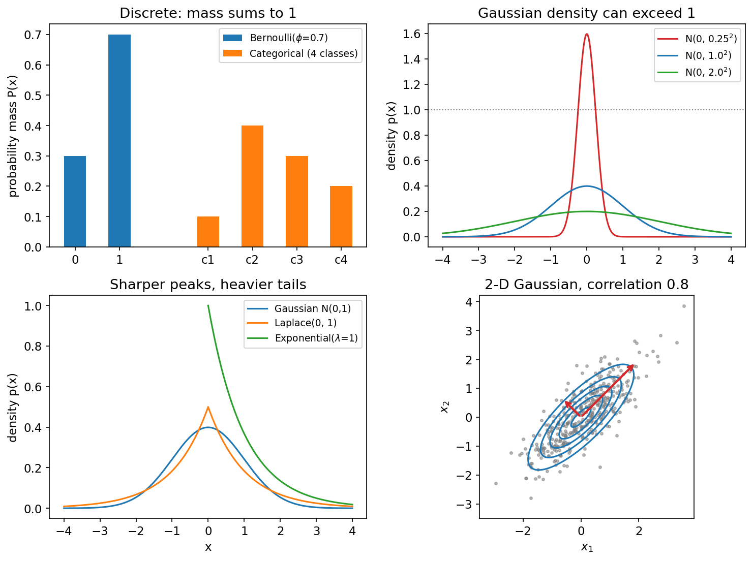
The probability of any single exact value is zero. Because only areas must be at most one, a density can exceed one: a narrow Gaussian with standard deviation peaks at about (Figure 1, top right). A common mistake is to report “probability 1.6” for a density value.
Marginal probability
Plain version. If you know how two things vary together, you can recover how one of them varies on its own by “summing out” the other.
Given a joint distribution over and , the marginal distribution of is
This is the sum rule. If the joint is written as a table with rows for and columns for , the marginal of is the row sums — historically written in the margin of the page, hence the name.
Conditional probability
Plain version. A conditional probability answers “how likely is this, given that I already know that?”
is the probability of after we have observed . It is only defined when the condition can actually happen. Rearranging gives the product rule .
Do not confuse conditioning with intervention. “The probability that the street is wet given that people carry umbrellas” is high, but forcing people to carry umbrellas will not wet the street. Questions about interventions belong to causal inference, which needs more than a joint distribution.
The chain rule of probability
Applying the product rule repeatedly factorizes any joint distribution over variables:
Here is the value of the -th variable. This identity is exact — no assumption is involved. It is the backbone of autoregressive models: a language model or an autoregressive image model predicts one token or pixel at a time given all previous ones (ML 09, NLP 01). The modelling choice lies in how each conditional is parameterized, not in the factorization itself.
Independence and conditional independence
Two variables are independent, written , if
They are conditionally independent given , written , if
Ice-cream sales and sunburn are dependent, but roughly independent once you condition on the weather. Conditional independence is the main tool for making high-dimensional models tractable — naive Bayes assumes the features are independent given the class; a hidden Markov model assumes the future is independent of the past given the present state. These are assumptions [3]: they should be justified by the problem, not adopted only because they make the algebra easy.
Code: a joint table, marginals and conditionals
The following example builds a small joint table for weather and umbrella use, computes marginals and conditionals, and tests independence. It also shows a case where two variables are clearly dependent yet have (almost) zero covariance.
Code · Python · 20 lines
import numpy as np

# Joint table P(weather, umbrella): rows = sunny/rainy, columns = no/yes
P = np.array([[0.56, 0.14],
              [0.06, 0.24]])
assert np.isclose(P.sum(), 1)

p_weather = P.sum(axis=1)            # marginal over umbrella
p_umbrella = P.sum(axis=0)           # marginal over weather
p_umb_given_w = P / p_weather[:, None]   # each row sums to 1
print("P(weather):", p_weather)
print("P(umbrella):", p_umbrella)
print("P(umbrella | weather):\n", p_umb_given_w)
print("independent?", np.allclose(P, np.outer(p_weather, p_umbrella)))

# Zero covariance does not imply independence
rng = np.random.default_rng(0)
x = rng.uniform(-1, 1, 200_000)
y = x**2                              # y is a deterministic function of x
print("cov(x, y) ~", np.cov(x, y)[0, 1].round(4))
Output: the marginals are and ; the conditional table is ; the variables are not independent; and the sample covariance of and is about , essentially zero, even though is completely determined by .
Expectation, variance and covariance
Plain version. The expectation is the long-run average; the variance is how far values typically spread from that average; the covariance says whether two quantities tend to go up and down together.
The expectation of a function under a distribution is
The subscript names the distribution we average over; we drop it when it is obvious. Expectation is linear: for constants . Almost every training loss is an expectation over the data distribution, estimated by an average over a mini-batch.
The variance measures spread around the mean :
Its square root is the standard deviation, which has the same units as .
The covariance of two quantities measures how they vary together:
A positive covariance means both tend to be above (or below) their means at the same time; a negative covariance means one tends to be high when the other is low. Its magnitude depends on the units, so we often normalize it into the correlation
Independence implies zero covariance, but zero covariance does not imply independence. Covariance measures only linear dependence. In the code above, with uniform on : knowing tells you exactly, but the covariance is zero because the relationship is symmetric and nonlinear. Mutual information, introduced later, captures every kind of dependence.
The covariance matrix
For a random vector with mean , the covariance matrix is
Its diagonal holds the variances . is symmetric and positive semidefinite, so (by ML 01A) it has real nonnegative eigenvalues and orthogonal eigenvectors. The eigenvectors are the principal axes of the data cloud and the eigenvalues are the variances along them — the red arrows in Figure 1 — which is exactly what PCA computes. For an affine map , and .
Common probability distributions
Plain version. A handful of distributions appear over and over. Choosing one is choosing an assumption about your data or your target.
Bernoulli
A single binary variable with parameter :
Its mean is and its variance . A binary classifier with a sigmoid output predicts the parameter of a Bernoulli distribution over the label.
Categorical (multinoulli)
A single discrete variable with states, parameterized by a probability vector with :
If the label is encoded one-hot as , then . A softmax classifier outputs exactly such a vector. (The multinomial distribution counts outcomes over several draws; for one draw it reduces to the categorical, which Goodfellow et al. call “multinoulli” [1].)
Gaussian (normal)
The most widely used continuous distribution:
is the mean (and the peak), the variance. Sometimes we use the precision instead, which is cheaper to evaluate when the variance changes often.
Two reasons make the Gaussian the default. The central limit theorem says that the sum of many independent variables with finite variance tends towards a Gaussian, so measurement noise built from many small effects is often near-Gaussian. And among all distributions with a given mean and variance on the real line, the Gaussian has the maximum entropy: it builds in the least extra structure.
In dimensions,
where is the mean vector and is a symmetric positive-definite covariance matrix. The precision matrix has a neat meaning: exactly when and are conditionally independent given all other coordinates. An isotropic Gaussian has — the noise distribution used by diffusion models (ML 08).
A fundamental link to the losses you will use: if a regression network predicts the mean of a Gaussian with fixed variance, maximizing the likelihood is the same as minimizing the mean squared error.
Exponential and Laplace
Sometimes we want a sharp point at a specific location.
is the rate, is the indicator that is 1 when and 0 otherwise, is the location and the scale. Compared with the Gaussian, the Laplace density has a sharper peak and heavier tails (Figure 1, bottom left). Predicting the location of a Laplace distribution by maximum likelihood is equivalent to minimizing the absolute error ( loss), which is why is more tolerant of outliers than ; a Laplace prior on weights gives regularization (sparsity).
Dirac and empirical distributions
The Dirac delta puts all of its mass at the point : it is zero everywhere else yet integrates to one. It is a generalized function, defined by what it does inside integrals: .
A training set defines the empirical distribution
which puts mass on each of the examples. Training a model by averaging a loss over the dataset is the same as taking an expectation under . It is also the distribution that maximizes the likelihood of the training data — which is precisely why minimizing training loss alone overfits.
Mixtures and latent variables
Plain version. A mixture first picks a “type” at random, then draws a sample from the distribution belonging to that type.
is a categorical latent variable — a variable we never observe directly — chosen with probabilities , and is the -th component. A Gaussian mixture model (GMM) uses Gaussian components ; with enough components it can approximate any smooth density to any desired nonzero error [1]. Given an observation , Bayes’ rule gives the posterior responsibility : how likely it is that component generated that point. Fitting a GMM with expectation–maximization is the subject of PR 07.
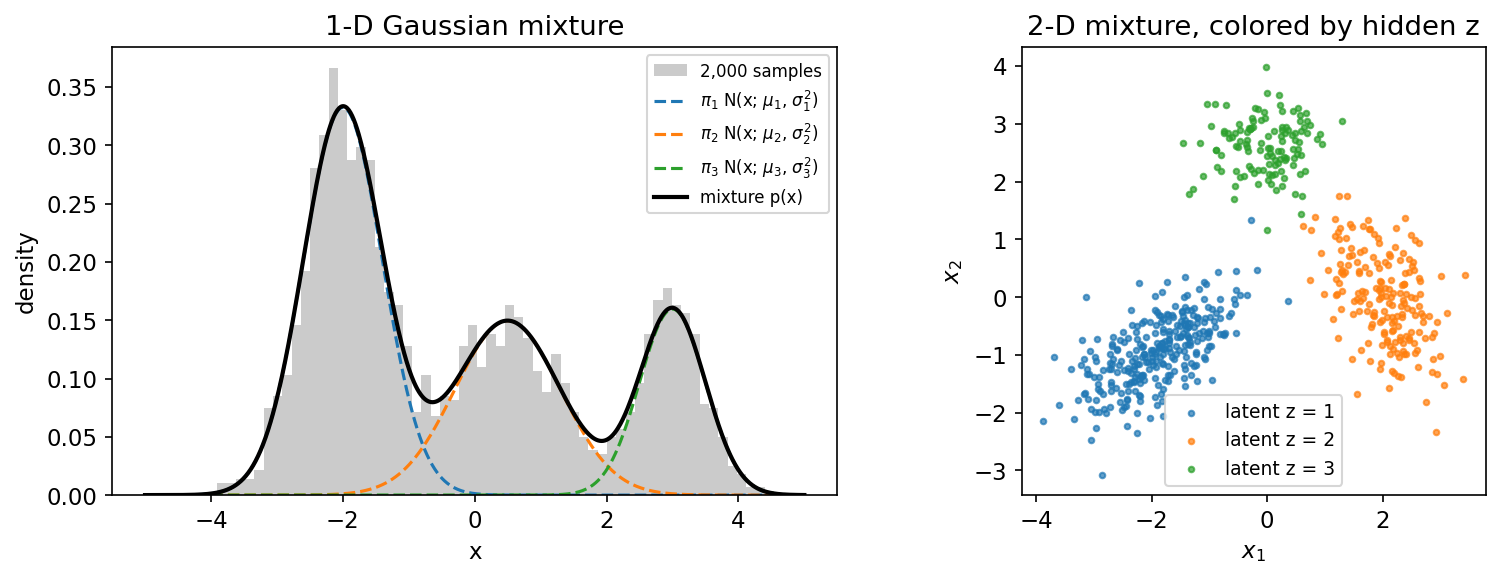
Latent variables are central to modern generative models. A VAE (ML 07) is, informally, a mixture with a continuous latent and a neural network for [8]; the marginal is then intractable and must be approximated.
Code · Python · 27 lines
import numpy as np

rng = np.random.default_rng(0)
pi = np.array([0.5, 0.3, 0.2])      # mixing weights P(z = k)
mu = np.array([-2.0, 0.5, 3.0])     # component means
sd = np.array([0.6, 0.8, 0.5])      # component standard deviations

# Ancestral sampling: first the hidden component z, then x given z
z = rng.choice(3, size=100_000, p=pi)
x = rng.normal(mu[z], sd[z])

def log_normal(x, m, s):
    return -0.5*((x - m)/s)**2 - np.log(s) - 0.5*np.log(2*np.pi)

def mixture_logpdf(x):
    # log sum_k pi_k N(x; mu_k, sd_k^2), computed with log-sum-exp
    a = np.log(pi) + log_normal(x[:, None], mu, sd)
    m = a.max(axis=1, keepdims=True)
    return (m + np.log(np.exp(a - m).sum(axis=1, keepdims=True))).ravel()

grid = np.linspace(-6, 6, 4001)
print("density integrates to", (np.exp(mixture_logpdf(grid)).sum()*(grid[1]-grid[0])).round(4))
print("sample mean", x.mean().round(3), "vs exact", (pi*mu).sum().round(3))
# Posterior responsibility P(z | x) for one observation
a = np.log(pi) + log_normal(np.array([0.0])[:, None], mu, sd)
resp = np.exp(a - a.max()); resp /= resp.sum()
print("P(z | x=0):", resp.round(3))
The density integrates to 1.0, the sample mean (−0.255) matches the exact mean , and the point is assigned to the middle component with probability 0.99. The log-sum-exp trick used here is explained in ML 01C.
Useful functions: sigmoid and softplus
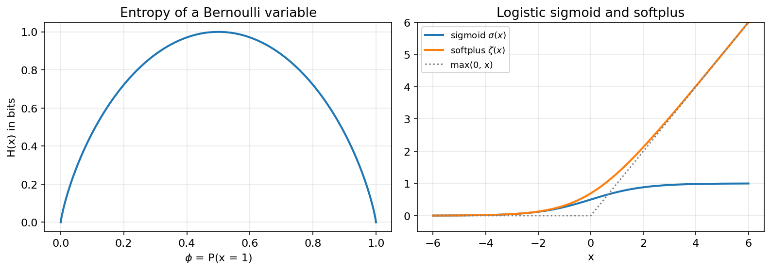
Plain version. The sigmoid squashes any real number into a probability between 0 and 1; the softplus is a smooth version of that is always positive.
The logistic sigmoid produces the parameter of a Bernoulli distribution; it saturates (becomes flat) for large , which makes gradients small there. The softplus produces a positive number, such as a standard deviation or a precision ; its name comes from being a softened “positive part” .
These identities are worth memorizing, because they appear every time a loss is simplified [1]:
is the logit (log-odds) function. The identity shows why binary cross-entropy should be computed from logits: , and softplus can be evaluated without overflow.
Code · Python · 18 lines
import numpy as np

def sigmoid(x):
    return 1/(1 + np.exp(-x))

def softplus(x):
    return np.logaddexp(0, x)          # log(1 + exp(x)) without overflow

x = np.linspace(-30, 30, 13)
assert np.allclose(1 - sigmoid(x), sigmoid(-x))
assert np.allclose(np.log(sigmoid(x)), -softplus(-x))
assert np.allclose(softplus(x) - softplus(-x), x)
h = 1e-6
assert np.allclose((softplus(x+h) - softplus(x-h))/(2*h), sigmoid(x), atol=1e-6)
p = sigmoid(x[4:9])
assert np.allclose(np.log(p/(1-p)), x[4:9])   # logit inverts sigmoid
print("naive log(1+exp(1000)):", np.log1p(np.exp(np.float64(1000))))
print("stable softplus(1000):", softplus(1000.0))
All identities pass. The naive expression returns inf (with an overflow warning) while np.logaddexp returns 1000.0.
Bayes’ rule
Plain version. Bayes’ rule combines how well a hypothesis explains the evidence with how plausible it was beforehand.
From the product rule written both ways, , so
- is the prior: how plausible is before seeing the evidence.
- is the likelihood of the evidence under hypothesis .
- is the posterior: the updated plausibility.
- is the evidence (or marginal likelihood), the normalizer obtained by summing over all hypotheses .
A worked example: the base-rate effect
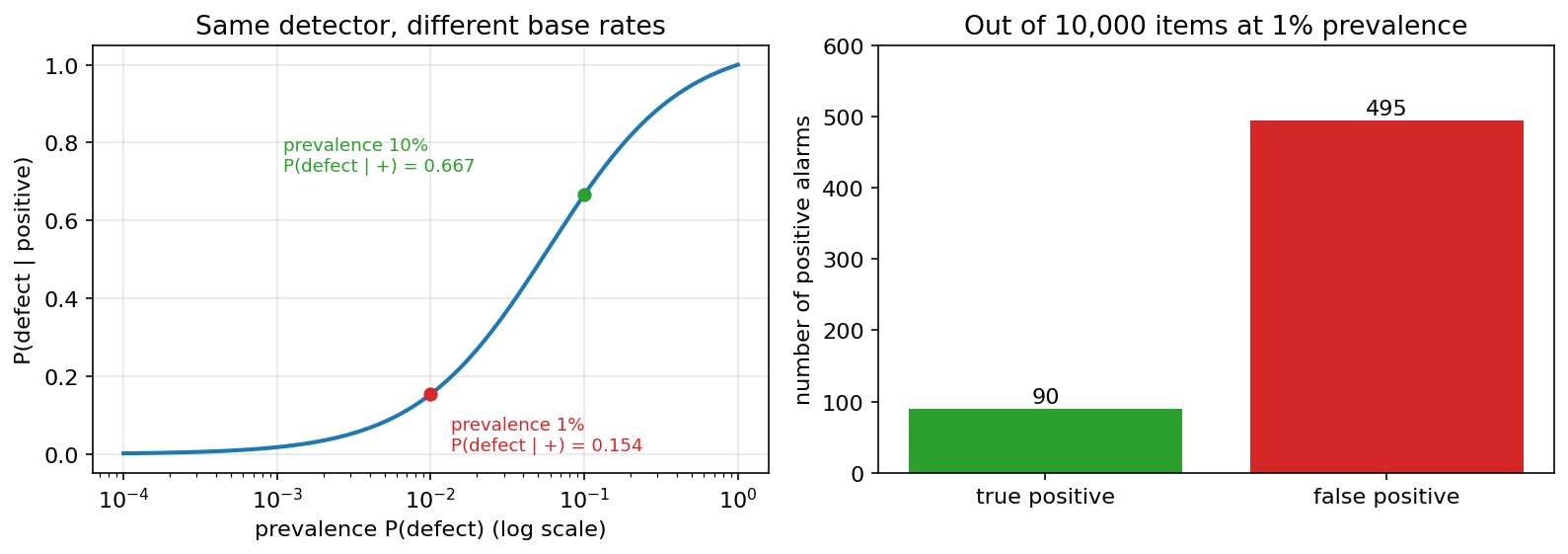
Consider a hypothetical defect detector with sensitivity , false-positive rate , and a prevalence (base rate) . The probability that an item flagged as positive really is defective is
Only about 15% of alarms are real, even though the detector catches 90% of defects. Counting makes this obvious: among 10,000 items, 100 are defective and 90 of them raise an alarm, but 9,900 are fine and 495 of them also raise an alarm (Figure 4, right). The same detector at 10% prevalence gives . This is a mathematical illustration, not a performance claim about any real system. Its lesson carries over to every deployed classifier: sensitivity and false-positive rate alone do not determine how trustworthy a positive prediction is; the deployment prevalence matters. ML 11 returns to this when discussing precision under distribution shift.
Code · Python · 14 lines
import numpy as np

def posterior_positive(prevalence, sensitivity=0.9, false_pos=0.05):
    evidence = sensitivity*prevalence + false_pos*(1 - prevalence)   # P(+)
    return sensitivity*prevalence / evidence                          # P(defect | +)

for prev in [0.001, 0.01, 0.1, 0.5]:
    print(f"prevalence {prev:>5}: P(defect | +) = {posterior_positive(prev):.3f}")

# Simulation check with 1,000,000 synthetic items
rng = np.random.default_rng(0)
defect = rng.random(1_000_000) < 0.01
alarm = np.where(defect, rng.random(defect.size) < 0.9, rng.random(defect.size) < 0.05)
print("simulated:", defect[alarm].mean().round(3))
The formula gives 0.018, 0.154, 0.667 and 0.947 for the four prevalences, and a one-million-item simulation reproduces 0.154.
Bayes’ rule also underlies the Bayes classifier: predicting the class with the largest posterior minimizes the expected error rate. PR 01 develops this decision theory in depth.
Change of variables for densities
Plain version. If you stretch a rubber sheet, the ink on it gets thinner. When a random variable is transformed, its density must be rescaled by how much the transformation stretches space.
A tempting mistake: if and has density , then . This is wrong, because it does not integrate to one. The correct rule for an invertible, differentiable in one dimension is
The probability in a small interval must be preserved: . In dimensions, with ,
where is the Jacobian matrix of (entry is ) and is the absolute value of its determinant — the factor by which scales a small volume (see ML 01A for determinants). This formula is the entire foundation of normalizing flows, which stack invertible networks with cheap Jacobian determinants to obtain an exact likelihood [9].
Code · Python · 18 lines
import numpy as np

rng = np.random.default_rng(0)
x = rng.normal(0, 1, 500_000)        # x ~ N(0, 1)
y = np.exp(x)                        # y = g(x), invertible on (0, inf)

def p_x(x):
    return np.exp(-0.5*x**2)/np.sqrt(2*np.pi)

def p_y(y):
    # p_y(y) = p_x(g^{-1}(y)) * |d g^{-1}(y) / dy| = p_x(log y) / y
    return p_x(np.log(y))/y

counts, edges = np.histogram(y, bins=np.linspace(0.05, 4, 80), density=False)
centers = 0.5*(edges[:-1] + edges[1:])
empirical = counts/(y.size*np.diff(edges))
print("max |histogram - formula|:", np.abs(empirical - p_y(centers)).max().round(3))
print("wrong formula (no Jacobian) error:", np.abs(empirical - p_x(np.log(centers))).max().round(3))
With the Jacobian factor the histogram matches the formula to within 0.011 (sampling noise); without it the error is 0.46.
Likelihood, maximum likelihood and MAP
Plain version. Hold the observed data fixed and ask which parameter values make that data most plausible. If you also have prior knowledge about the parameters, weigh that in too.
Suppose a model has parameters , and we observe a dataset of independent and identically distributed (i.i.d.) examples. The likelihood is
As a function of , this is not a probability distribution over parameters: it need not integrate to one over . The maximum likelihood estimate (MLE) is
We take logarithms because a product of many numbers below one underflows, while a sum of logs is numerically safe and has the same maximizer. The right-hand form says MLE minimizes the average negative log-likelihood (NLL) under the empirical distribution . For a classifier the same idea gives the conditional NLL , which is the cross-entropy loss we meet below.
Two classic results: for a Bernoulli coin with heads in flips, ; for a Gaussian, is the sample mean and — a slightly biased estimate (dividing by removes the bias).
MAP estimation
Bayesian inference treats itself as a random variable with a prior and computes the posterior
The full posterior is often intractable, so a common shortcut is its mode, the maximum a posteriori (MAP) estimate:
With a Gaussian prior , the term equals plus a constant: weight decay is MAP with a Gaussian prior. A Laplace prior gives regularization. This links probabilistic assumptions to the regularizers in ML 02. But a MAP point estimate is still a single parameter vector; it does not tell you how uncertain the parameters are. Approximating the whole posterior is the topic of PR 08 and of variational inference [10].
Code · Python · 20 lines
import numpy as np

rng = np.random.default_rng(0)
flips = rng.random(10) < 0.7          # 10 coin flips, true P(heads) = 0.7
k, n = flips.sum(), flips.size

phi = np.linspace(1e-3, 1 - 1e-3, 999)
log_lik = k*np.log(phi) + (n - k)*np.log(1 - phi)
a, b = 5.0, 5.0                        # Beta(5, 5) prior, centered on 0.5
log_prior = (a - 1)*np.log(phi) + (b - 1)*np.log(1 - phi)

print(f"{k} heads in {n} flips")
print("MLE  grid:", phi[log_lik.argmax()].round(3), " closed form:", k/n)
print("MAP  grid:", phi[(log_lik + log_prior).argmax()].round(3),
      " closed form:", round((k + a - 1)/(n + a + b - 2), 3))

# Gaussian MLE: sample mean and the 1/m (biased) variance
x = rng.normal(2.0, 3.0, 50)
print("Gaussian MLE mean, var:", x.mean().round(3), x.var().round(3),
      " unbiased var:", x.var(ddof=1).round(3))
With this seed, 6 heads appear in 10 flips. The MLE is 0.6; the Beta(5, 5) prior pulls the MAP estimate towards 0.5, giving 0.556, matching the closed form . With more data the likelihood dominates and the two estimates converge. The Gaussian MLE variance (7.71) is smaller than the unbiased estimate (7.87), as expected.
Information theory
Plain version. Information theory measures surprise. A rare event carries a lot of information when it happens; a certain event carries none. Averaging surprise gives entropy, and the extra surprise from using the wrong distribution gives KL divergence.
Claude Shannon founded the field to study how many bits are needed to send messages over a noisy channel [5]; the textbook treatment is Cover and Thomas [7]. For machine learning, the useful idea is to quantify how different two distributions are.
Self-information and entropy
The self-information of an outcome is
With the natural logarithm the unit is the nat; with it is the bit (one nat bits). Certain events () carry zero information; unlikely events carry a lot; and information from independent events adds, because logs turn products into sums.
The Shannon entropy is the expected self-information:
We use the convention , justified by the limit as . Entropy is the minimum average number of bits (or nats) needed to encode outcomes drawn from . It is zero for a deterministic outcome and maximal, , for a uniform distribution over outcomes. For a Bernoulli variable with parameter , , which peaks at one bit when (Figure 3, left).
For continuous variables, is the differential entropy. Treat it carefully: it can be negative (a narrow uniform distribution on has ) and it changes when you rescale the coordinates. It is not a limiting version of the discrete count of bits.
KL divergence
The Kullback–Leibler divergence [6] measures how different a distribution is from a reference :
In coding terms, it is the extra number of nats needed to encode samples from when the code was designed for . Its key properties:
- Nonnegative: , with equality if and only if (for discrete variables; “almost everywhere” for continuous ones). This follows from Jensen’s inequality, because is convex.
- Infinite under unsupported mass: if for some with , the divergence is infinite.
- Asymmetric: in general , and it does not satisfy the triangle inequality. KL is therefore not a distance metric, even though it is often described as “the distance between distributions”.
Forward versus reverse KL
The asymmetry has visible consequences when the approximating family is too simple. Figure 5 fits a single Gaussian to a target with two well-separated modes.
- Minimizing forward KL heavily penalizes for being small where has mass. The best Gaussian therefore covers both modes, placing its mean between them (, ) and putting a lot of mass in the empty valley. For Gaussian , the forward-KL optimum simply matches the mean and variance of .
- Minimizing reverse KL heavily penalizes for being large where is small. The best Gaussian therefore locks onto one mode (, ) and ignores the other.
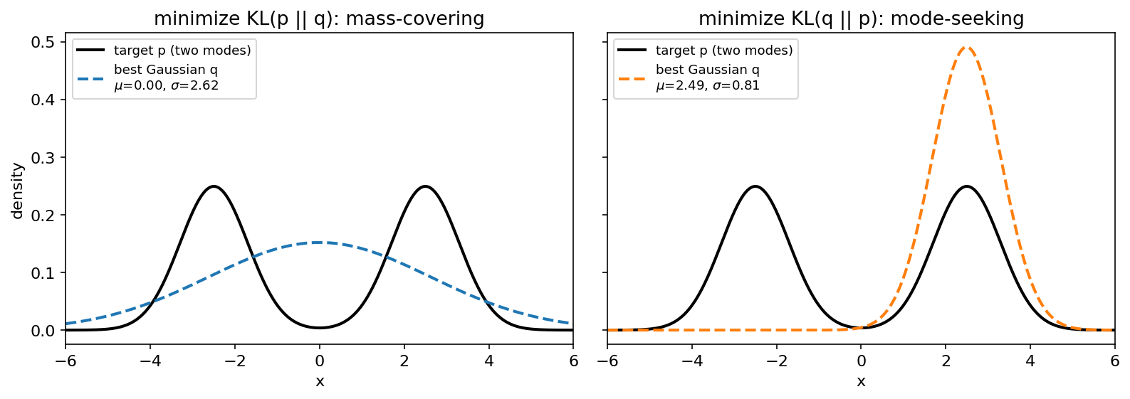
Which direction you minimize is a design choice. Maximum likelihood minimizes forward KL from the data distribution to the model, so likelihood-trained models (autoregressive models, flows, VAEs) tend to spread probability over all the data, sometimes producing blurry samples. Variational inference usually minimizes reverse KL from the approximation to the true posterior [10], and so tends to underestimate posterior uncertainty.
Cross-entropy
The cross-entropy of relative to is
Because does not depend on , minimizing cross-entropy with respect to is the same as minimizing forward KL. In classification, is the empirical label distribution — a one-hot vector for each example — and is the model’s softmax output . For one example with true class ,
where is the one-hot vector for class . Averaged over a dataset, this is exactly the conditional negative log-likelihood. So “cross-entropy loss”, “log loss” and “negative log-likelihood of a categorical model” are three names for the same objective. Any loss consisting of a negative log-likelihood is a cross-entropy between the empirical distribution and the model — which is why the mean squared error is also “the cross-entropy” for a Gaussian model [1].
Mutual information
Mutual information measures how much knowing one variable reduces uncertainty about another:
Here is the conditional entropy and the joint entropy. , with equality if and only if and are independent — unlike covariance, it detects any form of dependence. It is symmetric in and .
Code: information quantities
Code · Python · 26 lines
import numpy as np

p = np.array([.7, .2, .1])
q = np.array([.5, .3, .2])
entropy = -(p*np.log(p)).sum()
cross_entropy = -(p*np.log(q)).sum()
kl = (p*np.log(p/q)).sum()
reverse_kl = (q*np.log(q/p)).sum()
assert np.allclose(cross_entropy - entropy, kl) and kl >= 0
print("H(p), H(p,q), KL(p||q), KL(q||p) in nats:",
      np.round([entropy, cross_entropy, kl, reverse_kl], 4))
print("H(p) in bits:", (entropy/np.log(2)).round(4))

# Mutual information from a joint table (same weather/umbrella table)
P = np.array([[0.56, 0.14],
              [0.06, 0.24]])
px, py = P.sum(1), P.sum(0)
mi = (P*np.log(P/np.outer(px, py))).sum()
H = lambda t: -(t[t > 0]*np.log(t[t > 0])).sum()
assert np.isclose(mi, H(px) + H(py) - H(P.ravel()))
print("I(weather; umbrella) =", mi.round(4), "nats")

# Cross-entropy loss on one-hot labels equals mean -log q(y)
probs = np.array([[0.7, 0.2, 0.1], [0.1, 0.8, 0.1], [0.3, 0.3, 0.4]])
labels = np.array([0, 1, 2])
print("mean cross-entropy:", (-np.log(probs[np.arange(3), labels])).mean().round(4))
Output: , , and nats — the two directions differ. is 1.1568 bits. The weather–umbrella mutual information is 0.1637 nats, and both formulas for it agree. The mean cross-entropy of the three predictions is 0.4987 nats. In real training code, compute the cross-entropy from logits with a fused function rather than from probabilities (see ML 01C).
Optional: Shannon (in the Paper guides). Read the original figure, evidence, design choices and limitations.
Structured probabilistic models
Plain version. Graphical models use conditional-independence structure to factor a joint distribution into smaller pieces. The graph alone does not establish causation.
A joint table over 100 binary variables would need numbers. Structured probabilistic models, also called graphical models, exploit conditional independence to factorize the joint into small factors [1], [3]. There are two main kinds.
Directed models (Bayesian networks) use a directed acyclic graph . Each variable depends only on its parents :
For example, with and we have ; deleting the edge asserts and shortens the last factor to . Directed graphs are natural for generative stories (“first choose the class, then the pixels”), and a mixture model is the simplest example: .
Undirected models (Markov random fields) use an undirected graph. Each clique (a set of mutually connected nodes) has a nonnegative factor , and
The partition function normalizes the product; computing it is often the hard part. Undirected models suit symmetric interactions, like neighbouring pixels in an image prior or a conditional random field for segmentation.
A graph is a description of a distribution, not a different kind of distribution: any distribution can be written either way, although one may be much more compact. Deep learning often uses these ideas implicitly — an autoregressive model is a fully connected directed model, and a VAE is a two-node directed model whose conditional is a neural network [8].
Modern view
The probability and information theory in this chapter is classical. What has changed in the deep-learning era is how it is used and what goes wrong in practice. This section surveys the review literature and recent directions; it summarizes their framing rather than reproducing benchmark numbers.
Calibration: are predicted probabilities honest?
A classifier is calibrated if, among all inputs for which it predicts confidence 0.8, about 80% are correct. Guo et al. [11] (ICML 2017) found that modern deep networks are often overconfident, and identified depth, width, weight decay and batch normalization as factors that affect calibration. Their main recommendation, temperature scaling — dividing all logits by a single scalar fitted on a validation set — is a one-parameter variant of Platt scaling and remains a strong baseline because it changes confidence without changing the predicted class. Wang’s survey [12] organizes calibration methods into four families: post-hoc calibration, regularization during training, uncertainty estimation, and compositions of these; its revised version also covers calibration of large language models. The probabilistic lesson: a softmax output is a model of , and like any model it can be wrong in its uncertainty, not only in its argmax.
Uncertainty quantification
Two major reviews map the field of uncertainty in deep learning. Abdar et al. [13] (Information Fusion, 2021) review Bayesian approximations, ensembles and their applications across many domains. Gawlikowski et al. [14] (Artificial Intelligence Review, 2023) distinguish reducible model (epistemic) uncertainty from irreducible data (aleatoric) uncertainty — roughly the third and first sources of uncertainty from the start of this chapter — and compare deterministic single networks, Bayesian methods, ensembles and test-time augmentation, together with calibration measures.
Two primary studies are especially influential. Deep ensembles [15] train several networks from different random initializations and average their predictive distributions; this simple, parallel method was competitive with approximate Bayesian neural networks and expressed higher uncertainty on out-of-distribution inputs. Ovadia et al. [16] (NeurIPS 2019) benchmarked uncertainty methods under dataset shift and found that post-hoc calibration on in-distribution validation data did not carry over well, while methods that marginalize over models (such as ensembles) held up better.
A complementary, assumption-light approach is conformal prediction. Angelopoulos and Bates [17] give an accessible introduction: using a held-out calibration set, conformal methods turn any pre-trained model’s scores into prediction sets that contain the true label with a user-chosen probability, assuming the calibration and test data are exchangeable. It does not require the model’s probabilities to be calibrated, which makes it attractive for vision and language systems that are used as black boxes.
Mutual information in representation learning
Mutual information became a popular objective for self-supervised learning (ML 06). Contrastive Predictive Coding [18] introduced the InfoNCE loss, which classifies a positive pair among negatives and can be shown to maximize a lower bound on mutual information. Poole et al. [19] (ICML 2019) unified many variational MI bounds and showed that they degrade when the true MI is large, trading high bias against high variance. Tschannen et al. [20] (ICLR 2020) argued that the success of these methods “cannot be attributed to the properties of MI alone”: the encoder architecture and the parameterization of the estimator matter at least as much. The modern consensus is to treat InfoNCE-style objectives as well-behaved contrastive losses with an information-theoretic motivation, not as precise MI estimators.
Divergences and latent variables in generative models
Generative modelling is applied probability. VAEs [8] maximize an evidence lower bound that combines a reconstruction likelihood with a KL term; Blei et al. [10] review variational inference, which approximates intractable posteriors by minimizing (reverse) KL within a tractable family. Normalizing flows [9] are built entirely on the change-of-variables formula. Diffusion and flow-matching models (ML 08) combine Gaussian noise, conditional expectations and likelihood bounds. The choice of divergence (forward KL, reverse KL, or something else) shapes whether a model covers all the data or concentrates on its modes — the same picture as Figure 5, at scale.
Open problems
- Calibration under shift. Calibration that holds on a validation set can fail on new cameras, hospitals or prompts [16]; detecting when this happens is an open question.
- Separating uncertainty types. Decomposing predictive uncertainty into epistemic and aleatoric parts is conceptually clear but hard to do reliably for large networks [14].
- Estimating information in high dimensions. Variational MI bounds have fundamental bias–variance limits [19], so information-theoretic claims about deep representations need care.
- Uncertainty for foundation models. Applying calibration and conformal methods to large vision–language and language models, whose outputs are open-ended, is an active research area [12], [17].
Key takeaways
- Discrete probabilities sum to one; continuous densities integrate to one and may exceed one at a point.
- Marginalization and the chain rule are identities; independence is an additional assumption.
- Zero covariance does not generally imply independence.
- Likelihood and prior assumptions determine the resulting loss and regularization; keep their scale parameters explicit.
- Bayes’ rule updates prior beliefs with evidence; density transformations also require a volume correction.
- Cross-entropy separates into entropy and KL. KL is asymmetric; mode-covering or mode-seeking behavior depends on the approximation family and problem.
Exercises
- Units and certainty. (a) Convert a loss of 1 nat into bits. (b) Compute the entropy, in bits, of a fair coin, a certain outcome, and a fair 8-sided die.
Hint
(a) Divide by : about 1.443 bits. (b) 1 bit, 0 bits and bits. A uniform distribution over outcomes has entropy , the maximum for outcomes.
- Prevalence shift. Using the detector in the Bayes section, find the prevalence at which a positive result is exactly a coin flip, .
Hint
Set , where is the prevalence. Then , about 5.3%. Below that, most alarms are false.
- Dependent but uncorrelated. Let take values with equal probability and . Show that and compute in bits.
Hint
and , so the covariance is zero. Because is a function of , and . with probability and with probability , so bits.
- Gaussian MLE equals squared error. Show that maximizing over (with fixed) is equivalent to minimizing the mean squared error. What changes if is also predicted by the network?
Hint
The negative log-likelihood is . With fixed only the squared error depends on . If the network also predicts (for example through a softplus), each example’s error is weighted by and a penalty prevents the variance from growing without bound — a heteroscedastic regression model.
- Change of variables. If (uniform) and with , what is the density of ? Check your answer by sampling in NumPy.
Hint
and , while on . So for : the exponential distribution. This is the inverse-transform sampling trick.
- KL direction. For and , compute and . Which one is infinite, and what does that tell you about training a model by maximum likelihood?
Hint
nats (the third term is ). because puts mass where has none. Maximum likelihood minimizes , which becomes infinite if the model assigns zero probability to any observed example — so likelihood-trained models must spread some probability everywhere the data might be.
References
- I. Goodfellow, Y. Bengio and A. Courville, Deep Learning, MIT Press, 2016, ch. 3 “Probability and Information Theory”. Book
- C. M. Bishop and H. Bishop, Deep Learning: Foundations and Concepts, Springer, 2024. Book
- K. P. Murphy, Probabilistic Machine Learning: An Introduction, MIT Press, 2022. Book
- M. P. Deisenroth, A. A. Faisal and C. S. Ong, Mathematics for Machine Learning, Cambridge University Press, 2020. Book
- C. E. Shannon, “A Mathematical Theory of Communication,” Bell System Technical Journal, vol. 27, pp. 379–423, 1948. DOI
- S. Kullback and R. A. Leibler, “On Information and Sufficiency,” The Annals of Mathematical Statistics, vol. 22, pp. 79–86, 1951. DOI
- T. M. Cover and J. A. Thomas, Elements of Information Theory, 2nd ed., Wiley, 2006. DOI
- D. P. Kingma and M. Welling, “Auto-Encoding Variational Bayes,” in Proc. International Conference on Learning Representations (ICLR), 2014. arXiv
- G. Papamakarios, E. Nalisnick, D. J. Rezende, S. Mohamed and B. Lakshminarayanan, “Normalizing Flows for Probabilistic Modeling and Inference,” Journal of Machine Learning Research, vol. 22, no. 57, pp. 1–64, 2021. arXiv
- D. M. Blei, A. Kucukelbir and J. D. McAuliffe, “Variational Inference: A Review for Statisticians,” Journal of the American Statistical Association, vol. 112, no. 518, pp. 859–877, 2017. DOI
- C. Guo, G. Pleiss, Y. Sun and K. Q. Weinberger, “On Calibration of Modern Neural Networks,” ICML, 2017. arXiv
- C. Wang, “Calibration in Deep Learning: A Survey of the State-of-the-Art,” arXiv:2308.01222, 2023 (revised 2025). arXiv
- M. Abdar et al., “A Review of Uncertainty Quantification in Deep Learning: Techniques, Applications and Challenges,” Information Fusion, vol. 76, pp. 243–297, 2021. DOI
- J. Gawlikowski et al., “A Survey of Uncertainty in Deep Neural Networks,” Artificial Intelligence Review, vol. 56, pp. 1513–1589, 2023. DOI
- B. Lakshminarayanan, A. Pritzel and C. Blundell, “Simple and Scalable Predictive Uncertainty Estimation using Deep Ensembles,” NeurIPS (NIPS), 2017. arXiv
- Y. Ovadia et al., “Can You Trust Your Model’s Uncertainty? Evaluating Predictive Uncertainty Under Dataset Shift,” NeurIPS, 2019. arXiv
- A. N. Angelopoulos and S. Bates, “A Gentle Introduction to Conformal Prediction and Distribution-Free Uncertainty Quantification,” arXiv:2107.07511, 2021. arXiv
- A. van den Oord, Y. Li and O. Vinyals, “Representation Learning with Contrastive Predictive Coding,” arXiv:1807.03748, 2018. arXiv
- B. Poole, S. Ozair, A. van den Oord, A. A. Alemi and G. Tucker, “On Variational Bounds of Mutual Information,” ICML, 2019. arXiv
- M. Tschannen, J. Djolonga, P. K. Rubenstein, S. Gelly and M. Lucic, “On Mutual Information Maximization for Representation Learning,” ICLR, 2020. arXiv
Check your understanding
This tutorial has 6 exercises. Can you solve them without opening the hints?
Go to the exercises ↑Next ML 01C · Numerical Computation and Gradient Checks · 29 min