ML 04 · Recurrent and Recursive Networks
Needs: ML 02 · Neural Networks from Perceptron to Deep Networks
Navigate: this page and this track: Navigate: this page and this track
On this page
- What you’ll learn1 min
- The big picture2 min
- A recurrent state2 min
- Backpropagation through time1 min
- Vanishing and exploding gradients2 min
- Long short-term memory (LSTM)3 min
- Gated recurrent unit (GRU)1 min
- Deep, bidirectional and streaming RNNs1 min
- Encoder–decoder models and teacher forcing2 min
- Attention: the bridge to Transformers2 min
- Recurrent networks in vision1 min
- Recursive networks: composing over trees2 min
- Mamba: selective state spaces and scan3 min
- Modern view2 min
- Key takeaways1 min
- Exercises3 min
- Paper guides
- References
Machine Learning
Explore this chapter 1 interactive experiment
Compare a fixed recurrent decay with input-dependent write decisions while distractors pass through a sequence.
What you’ll learn
- Unroll recurrent updates and track shared parameters.
- Explain backpropagation through time and long-range gradient difficulties.
- Compare LSTM and GRU memory paths and gates.
- Distinguish bidirectional, sequence-to-sequence and tree-structured models.
- Assess attention and state-space alternatives for context, streaming and memory.
The big picture
ML 03 used one assumption about images: nearby pixels are related, and the same pattern can appear anywhere, so the same filter is reused across space. Sequences invite the same trick across time. A video is a sequence of frames, a caption is a sequence of words, a pen stroke is a sequence of positions. A recurrent neural network (RNN) reads such a sequence one element at a time, carries a summary called the hidden state from step to step, and uses the same weights at every step [1]. A recursive neural network generalizes the idea from a chain to a tree: it combines parts into wholes by repeatedly applying one shared composition rule.
Why study RNNs when Transformers dominate large-scale language and vision? Three reasons. First, every concept in modern sequence modeling — teacher forcing, encoder–decoder, attention, masking, causal generation — was developed on RNNs, and the Transformer is easiest to understand as the answer to RNN limitations. Second, recurrence is efficient for streaming: a constant-size state per step suits robots, sensors and on-device video. Third, recurrence is back: modern state-space models such as Mamba are recurrences with clever parameterizations, and ML 05 applies them to images.
A recurrent state
Plain version. At every step, combine the current input with the previous state to make a new state, using the same weights each time. Read outputs off the state whenever you need them.
Precise version. Let the input sequence be with , and let the hidden state be with a fixed starting state (usually zeros). The simple (Elman [9]) RNN is
maps the input into the state space, is the recurrent weight matrix that carries information from the previous step, and are biases, maps the state to outputs, and is an output function such as softmax. Crucially, none of these parameters depends on . That is parameter sharing across time, the temporal version of a CNN’s weight sharing: the model has the same number of parameters whether the sequence has 5 or 5,000 steps, and a pattern learned at step 3 can be recognized at step 300.
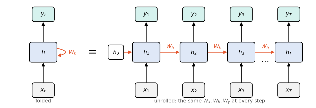
Unrolling (Figure 1) is the key mental move. Writing out the loop for steps produces an ordinary feed-forward network that is layers deep, in which every layer has the same weights. Everything you learned about backpropagation in ML 02 applies to this unrolled graph.
The same recurrence supports several input–output patterns:
| Pattern | Example | Output read from |
|---|---|---|
| Many-to-one | Classify a video clip; sentiment of a sentence | The last state (or a pooled state) |
| Many-to-many, aligned | Label every video frame; tag every word | Every |
| One-to-many | Generate a caption from one image vector | A decoder that feeds its own outputs back in |
| Many-to-many, unaligned | Translate a sentence; describe a video | An encoder–decoder (covered below) |
An RNN that predicts from is an autoregressive model, and sampling from it generates new sequences; but an RNN used as an encoder is not automatically a generator. The head and the loss decide the task.
Code: an RNN and its backward pass in NumPy
The snippet below implements the forward pass and backpropagation through time by hand for a loss , then checks one gradient entry against a finite difference. Notice the line dWh += …: because is used at every step, its gradient is the sum of contributions from all steps.
Code · Python · 36 lines
import numpy as np

rng = np.random.default_rng(0)
d, m, T = 3, 5, 7                                   # input size, state size, length
Wx = rng.normal(0, 0.5, (m, d))
Wh = rng.normal(0, 0.5, (m, m))
b = np.zeros(m)

def rnn_forward(xs, h0):
    hs = [h0]
    for x in xs:                                     # the SAME Wx, Wh, b at every step
        hs.append(np.tanh(Wx @ x + Wh @ hs[-1] + b))
    return hs

def rnn_backward(xs, hs, dhT):
    """BPTT for the loss L = dhT . h_T; returns dL/dWh and dL/dx_t for every t."""
    dWh, dxs, dh = np.zeros_like(Wh), [None] * len(xs), dhT
    for t in reversed(range(len(xs))):
        da = dh * (1 - hs[t + 1] ** 2)               # through tanh
        dWh += np.outer(da, hs[t])                   # shared weight: gradients ADD up
        dxs[t] = Wx.T @ da
        dh = Wh.T @ da                               # pass the gradient one step back
    return dWh, dxs

xs = rng.normal(size=(T, d))
hs = rnn_forward(xs, np.zeros(m))
dhT = rng.normal(size=m)
dWh, dxs = rnn_backward(xs, hs, dhT)

# finite-difference check of one entry of dL/dWh
eps, (i, j) = 1e-6, (2, 3)
Wh[i, j] += eps; up = dhT @ rnn_forward(xs, np.zeros(m))[-1]
Wh[i, j] -= 2 * eps; down = dhT @ rnn_forward(xs, np.zeros(m))[-1]
Wh[i, j] += eps
print("BPTT vs finite difference:", np.isclose(dWh[i, j], (up - down) / (2 * eps)))
print("|dL/dx_t| from first to last step:", np.round([np.linalg.norm(g) for g in dxs], 3))
It prints True, and the input-gradient norms are : even in a seven-step sequence, the early inputs receive gradients roughly ten to fifty times smaller than the late ones. That is the vanishing-gradient problem in miniature.
Backpropagation through time
Plain version. Unroll the network, run ordinary backpropagation through the unrolled graph, and add up the gradients for each shared weight.
Precise version. Write the pre-activation as , so . Suppose the loss is a sum over steps, . Working backward from , the total gradient arriving at is
The first term is the local loss at step ; the second is everything later that influenced, passed back one step. With (the gradient at the pre-activation), the parameter gradients are sums over time:
This algorithm, backpropagation through time (BPTT), was laid out clearly by Werbos [8]. Its cost is linear in , but so is its memory: every must be stored for the backward pass.
Truncated BPTT
For a very long stream (an hour of video, a continuous sensor log) storing all states is impossible. Truncated BPTT processes the stream in windows of steps. It carries the hidden state forward from one window to the next, so the model still sees the whole past, but it detaches the state from the graph at each window boundary, so gradients flow back at most steps. The model can therefore use long-range information only if it learns to preserve it from the gradient signal within windows.
Code · Python · 21 lines
import torch
from torch import nn

torch.manual_seed(0)
rnn, head = nn.GRU(1, 16, batch_first=True), nn.Linear(16, 1)
params = list(rnn.parameters()) + list(head.parameters())
opt = torch.optim.Adam(params, lr=1e-2)
t = torch.arange(0, 2000) * 0.05
stream = torch.sin(t) + 0.1 * torch.randn_like(t)   # one long noisy signal
x, y = stream[:-1, None][None], stream[1:, None][None]   # predict the next sample

h, window = None, 50
for start in range(0, x.shape[1] - window, window):
    out, h = rnn(x[:, start:start + window], h)
    loss = nn.functional.mse_loss(head(out), y[:, start:start + window])
    opt.zero_grad()
    loss.backward()                       # gradients flow back at most `window` steps
    nn.utils.clip_grad_norm_(params, 1.0)
    opt.step()
    h = h.detach()                        # keep the state, cut the graph
print("final window MSE:", round(loss.item(), 4), "(noise variance is 0.01)")
After a single pass over the stream, the final-window mean squared error is about 0.014, close to the 0.01 floor set by the added noise. Forgetting h.detach() makes the second window try to backpropagate into a graph that was already freed, and PyTorch raises an error; resetting h = None at each window instead would throw the context away.
Vanishing and exploding gradients
Plain version. Backpropagation multiplies state Jacobians across time. These products can shrink or grow sharply, making distant dependencies hard to learn.
Precise version. Chaining the one-step Jacobians gives
an ordered product of matrices (matrices do not commute, so the order matters). Because ,
where is the largest singular value. If , the gradient from distant steps vanishes exponentially. If has large singular values and the units are not saturated, the gradient can explode. Bengio, Simard and Frasconi [6] showed in 1994 that this is not a bug of a particular training method: a system that robustly stores information in the presence of noise must be in a regime where gradients of long-range dependencies shrink. Pascanu, Mikolov and Bengio [7] revisited the analysis with dynamical-systems tools and gave a practical remedy for explosions.
The intuition is clearest for a scalar linear RNN, : then , which is for and for . Figure 2 shows the same behavior measured in real networks.
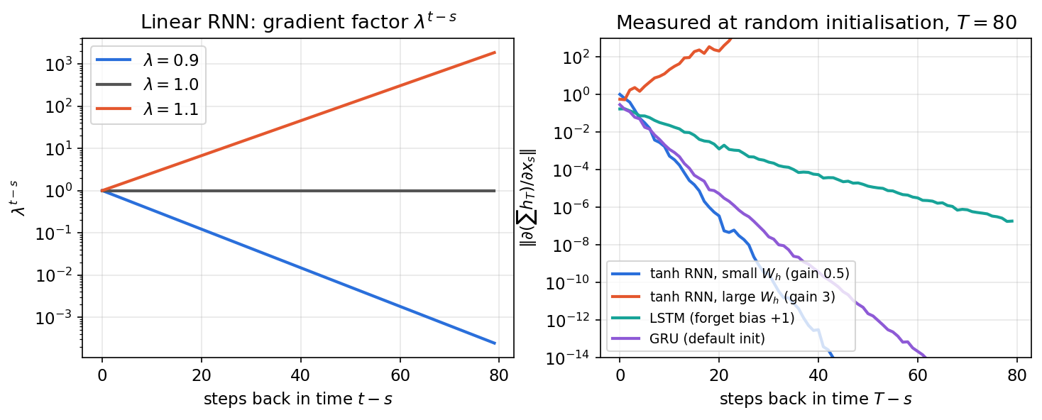
Remedies. Explosions are handled by gradient clipping [7]: if the gradient norm exceeds a threshold , rescale it to . This keeps the update direction and caps its length. PyTorch’s clip_grad_norm_ does exactly this. Vanishing gradients are harder: they require a different architecture, one whose state update is close to the identity so that gradients can pass through many steps. That architecture is the LSTM.
Long short-term memory (LSTM)
Plain version. Give the network a separate memory lane, the cell state, that is updated by addition rather than by repeated matrix multiplication, and let learned gates decide what to erase, what to write and what to reveal.
Precise version. With denoting concatenation and the logistic sigmoid, a standard LSTM step is
Each gate is a vector of numbers between 0 and 1, and is element-wise multiplication, so each gate acts like a bank of dimmer switches, one per memory unit. The forget gate decides how much of the old memory to keep, the input gate how much of the candidate to write, and the output gate how much of the memory to reveal as .
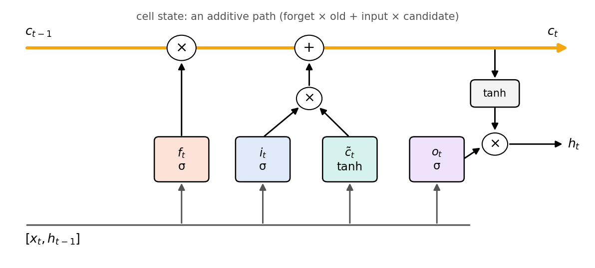
Why it works. Along the cell-state path, (ignoring the smaller indirect paths through the gates). There is no recurring weight matrix and no squashing nonlinearity on this path. If the forget gate stays near one, the gradient passes through many steps almost unchanged. That is why the LSTM curve in Figure 2 decays so slowly. It is also why a common initialization sets the forget-gate bias to a positive value such as , so the network starts out remembering. This is not a guarantee of unlimited memory: the forget gate can and does learn to close, and long-range credit assignment still gets harder with distance.
History and attribution. Hochreiter and Schmidhuber introduced the LSTM in 1997 [2] with a constant-error “carousel”: the cell state passed on unchanged and there was no forget gate. Gers, Schmidhuber and Cummins added the forget gate in 2000 [5] so that the cell could learn to reset its memory, for example between independent segments of a continuous stream. The equations above, with the forget gate, are the version used in practice and in every major framework. Greff et al. [19] compared eight LSTM variants on speech, handwriting and music tasks and found that none significantly beat the standard architecture, while the forget gate and the output activation were its most critical components.
Parameters. Each of the four gate blocks has an weight matrix and a bias, so an LSTM layer has about parameters, four times a simple RNN with the same state size. (PyTorch keeps separate input and recurrent biases, giving .)
Code: an LSTM step from scratch, checked against PyTorch
PyTorch stores the four gate blocks stacked in the order input, forget, cell candidate (), output. Implementing the step by hand and comparing with nn.LSTMCell is the best way to be sure you read the equations correctly:
Code · Python · 24 lines
import torch
from torch import nn

torch.manual_seed(0)
d, m = 4, 6
cell = nn.LSTMCell(d, m)                 # PyTorch stacks gate weights in order i, f, g, o

def lstm_step(x, h, c):
    z = x @ cell.weight_ih.T + cell.bias_ih + h @ cell.weight_hh.T + cell.bias_hh
    i, f, g, o = z.chunk(4, dim=-1)
    i, f, o = torch.sigmoid(i), torch.sigmoid(f), torch.sigmoid(o)
    g = torch.tanh(g)                    # candidate memory, often written c~_t
    c = f * c + i * g                    # additive cell update
    h = o * torch.tanh(c)
    return h, c

x = torch.randn(2, d)
h0, c0 = torch.randn(2, m), torch.randn(2, m)
h_ref, c_ref = cell(x, (h0, c0))
h_ours, c_ours = lstm_step(x, h0, c0)
print("matches nn.LSTMCell:", torch.allclose(h_ours, h_ref, atol=1e-6),
      torch.allclose(c_ours, c_ref, atol=1e-6))
print("parameters:", sum(p.numel() for p in cell.parameters()), "= 4 * m * (d + m + 2) =",
      4 * m * (d + m + 2))
It prints True True and 288 = … = 288.
Optional: LSTM (in the Paper guides). Read the original figure, evidence, design choices and limitations.
Gated recurrent unit (GRU)
Plain version. A GRU is a slimmer LSTM: it merges the cell and hidden states into one, and uses two gates instead of three.
Precise version. Following Cho et al. [3] and PyTorch’s nn.GRU,
The reset gate decides how much of the old state to use when forming the candidate; the update gate interpolates between keeping the old state () and replacing it (). The interpolation plays the role of the LSTM’s additive cell path. Two caveats are worth knowing. Some papers and textbooks swap the roles of and ; the models are equivalent, but the gate means the opposite. And the original paper applies the reset gate before the recurrent matrix (), whereas PyTorch and cuDNN apply it after, as written above. Always check the framework’s documentation before reading meaning into a gate.
GRUs have three gate blocks instead of four, so about 25% fewer parameters than an LSTM of the same width. Neither consistently wins across tasks; the GRU is a reasonable default when data or compute is limited.
Code: a recurrent classifier that generalizes to fresh sequences
This complete CPU example learns to classify the sign of a sequence’s sum, which requires accumulating information over all twelve steps. A fresh test set checks that the model did not merely memorize its training sequences.
Code · Python · 26 lines
import torch
from torch import nn
from torch.nn import functional as F

torch.manual_seed(0)
torch.set_num_threads(1)
rnn = nn.GRU(input_size=1, hidden_size=24, batch_first=True)
head = nn.Linear(24, 2)
opt = torch.optim.Adam(list(rnn.parameters())+list(head.parameters()), lr=.003)
def batch(n):
    x = torch.randn(n, 12, 1)
    y = (x.sum(dim=(1, 2)) > 0).long()
    return x, y
for step in range(400):
    x, y = batch(64)
    _, h = rnn(x)
    loss = F.cross_entropy(head(h[-1]), y)
    opt.zero_grad(); loss.backward()
    nn.utils.clip_grad_norm_(list(rnn.parameters())+list(head.parameters()), 1.)
    opt.step()
rnn.eval(); head.eval()
with torch.no_grad():
    x, y = batch(512)
    _, h = rnn(x)
    acc = (head(h[-1]).argmax(1) == y).float().mean()
    print("fresh-sequence accuracy:", acc.item())
It reaches about 99% accuracy on fresh length-12 sequences. The returned hidden tensor has shape layers × batch × hidden even with batch_first=True, which affects only the input and output sequence layout. Testing on longer sequences asks a different question, length generalization, and a model can succeed at length 12 and fail at length 100 (Exercise 2).
Deep, bidirectional and streaming RNNs
Stacking. A deep RNN feeds the sequence of hidden states of one recurrent layer into another (num_layers in PyTorch). Lower layers can capture short-range patterns and higher layers longer ones. Two to four layers are typical; deeper stacks usually need residual connections between layers.
Bidirectional. Schuster and Paliwal [10] proposed running one RNN forward in time and another backward, then concatenating their states, . Each position then summarizes both its past and its future. This is ideal for offline tasks where the whole input is available (tagging a recorded video, encoding a sentence), but it is not causal: it cannot be used for a live prediction that must be made before future frames arrive. Reporting offline bidirectional accuracy for an online application overstates what the deployed system can know.
Variable lengths. Batches contain sequences of different lengths, padded to a common length. Without care, the padding leaks into states and losses. Use per-sequence lengths (pack_padded_sequence in PyTorch) or masks so that padded steps neither update the state nor contribute to the loss.
Streaming. For a live stream, keep the state between calls and reset it only between independent streams. Accidentally carrying state from one user, document or video into the next leaks information and produces irreproducible results.
Encoder–decoder models and teacher forcing
Plain version. A basic encoder–decoder reads an input sequence into a state, then generates an output sequence from it. The two sequences can have different lengths.
Precise version. In the sequence-to-sequence (seq2seq) model of Sutskever, Vinyals and Le [11] and the closely related encoder–decoder of Cho et al. [3], an encoder RNN reads and its final state becomes a context vector . A decoder RNN, initialized from , models
where is the decoder state and is a softmax over the vocabulary. Generation stops when the decoder emits an end-of-sequence token, so input and output lengths are independent.
Teacher forcing. During training, the decoder input at step is the ground-truth previous token , not the model’s own prediction. This makes all steps trainable in parallel against the known target and greatly stabilizes learning. At test time, however, the model must consume its own predictions, which may contain errors it never saw during training. This train–test mismatch is called exposure bias. Scheduled sampling [25] gradually replaces ground-truth inputs with model samples during training to reduce it. Decoding usually uses greedy or beam search rather than sampling.
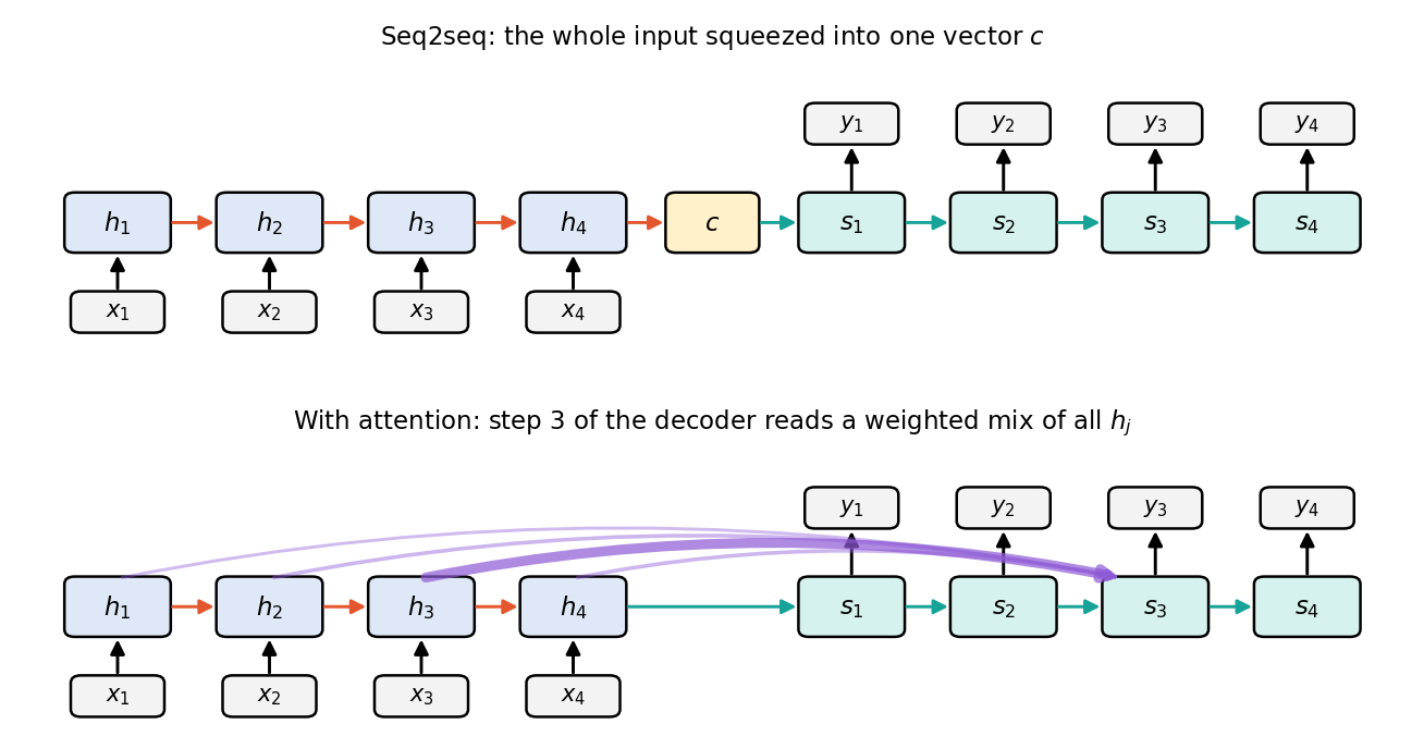
The weakness is visible in Figure 4 (top): everything the decoder knows about the input must pass through one fixed-size vector , no matter how long the input. Translation quality of plain seq2seq models dropped on long sentences. Sutskever et al. found that simply reversing the source sentence helped, because it shortened the distance between corresponding words, a hint that the bottleneck and long paths were the problem [11].
Attention: the bridge to Transformers
Plain version. Attention lets the decoder select relevant encoder states at each step instead of relying on one fixed summary.
Precise version. Bahdanau, Cho and Bengio [12] kept every encoder state (from a bidirectional encoder) and, at each decoder step , computed
is a learned alignment score between the decoder’s current need () and encoder position ; , and are learned parameters. The softmax turns scores into weights that are positive and sum to one, and the context vector is their weighted average of encoder states. The decoder then uses together with its own state. This form is called additive attention. Because changes at every step and has direct access to every input position, the path length between any input and any output becomes one step, regardless of the sequence length.
Code · Python · 29 lines
import torch
from torch import nn

class AdditiveAttention(nn.Module):
    """Bahdanau-style scores e_j = v^T tanh(W s + U h_j), then softmax over j."""
    def __init__(self, d_dec, d_enc, d_att):
        super().__init__()
        self.W = nn.Linear(d_dec, d_att, bias=False)
        self.U = nn.Linear(d_enc, d_att, bias=False)
        self.v = nn.Linear(d_att, 1, bias=False)

    def forward(self, s, H, mask=None):
        # s: B x d_dec (decoder state), H: B x T x d_enc (all encoder states)
        e = self.v(torch.tanh(self.W(s)[:, None] + self.U(H))).squeeze(-1)   # B x T
        if mask is not None:                       # True where the input is padding
            e = e.masked_fill(mask, float("-inf"))
        alpha = e.softmax(dim=-1)                  # attention weights, rows sum to 1
        context = (alpha[:, :, None] * H).sum(1)   # B x d_enc weighted average
        return context, alpha

torch.manual_seed(0)
att = AdditiveAttention(d_dec=16, d_enc=32, d_att=8)
H = torch.randn(2, 5, 32)
s = torch.randn(2, 16)
pad = torch.tensor([[False] * 5, [False, False, False, True, True]])   # 2nd sequence has length 3
ctx, alpha = att(s, H, pad)
print("context:", tuple(ctx.shape), "| weights sum to 1:",
      torch.allclose(alpha.sum(-1), torch.ones(2)))
print("weights on padding:", alpha[1, 3:].tolist())
It prints a context of shape (2, 32), confirms that weights sum to one, and shows exactly zero weight on padded positions: masking with before the softmax is the standard way to make attention ignore padding (and, in ML 05, the future).
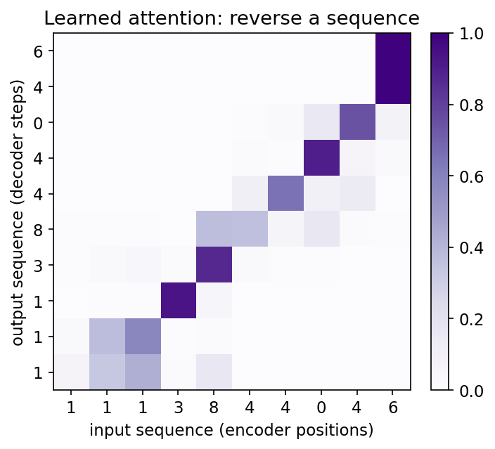
Attention weights are also interpretable as a soft alignment. Figure 5 shows a small GRU encoder–decoder with this attention trained for under a minute on CPU to reverse random digit sequences (about 96% per-token accuracy with teacher forcing on fresh sequences). Without being told, it learned to look at input position when writing output : the anti-diagonal.
From here to Transformers. Attention fixed the bottleneck, but the encoder and decoder were still recurrent, so computation over a sequence of length required sequential steps that cannot be parallelized during training. Vaswani et al. [28] asked what happens if recurrence is removed entirely and attention is used inside the encoder and decoder as well (self-attention), with positional encodings to restore order. The answer, the Transformer, trains in parallel across positions and became the dominant architecture for language and, with ViT, for vision. ML 05 picks up the story with scaled dot-product attention, which replaces the additive score with .
Recurrent networks in vision
Image captioning. Show and Tell [13] (Vinyals et al.) is a direct image-to-sequence model: a CNN (ML 03) encodes the image into a vector that initializes an LSTM language model, which then generates the caption word by word, trained with teacher forcing on image–caption pairs. Show, Attend and Tell [14] (Xu et al.) kept the CNN’s spatial feature grid instead of a single vector and let the LSTM attend over image regions at each word, producing attention maps that often highlight the object being named. This was one of the first widely seen demonstrations of visual attention.
Video understanding. Long-term Recurrent Convolutional Networks (LRCN) [15] (Donahue et al.) apply a CNN to each frame and an LSTM across frames, trained end to end, for activity recognition, image description and video description. The CNN handles space, the RNN handles time: a common pattern for any per-frame feature sequence, such as pose tracks or per-frame detections in object tracking.
Spatiotemporal forecasting. When the state itself should be an image, fully connected gates waste the spatial structure. The ConvLSTM of Shi et al. [16] replaces the matrix products in the LSTM gates with convolutions, , so inputs, states and gates are all 3-D tensors (channels × height × width). It was introduced for precipitation nowcasting from radar maps and is widely used for video prediction and other forecasting on grids.
What changed. For captioning and video classification at scale, Transformers and vision–language models (see ML 10) have largely replaced LSTMs, because they train in parallel and scale better with data. Recurrent and convolutional-recurrent models remain common where frames arrive one at a time and memory must stay constant: online video processing, tracking, robotics and low-power devices.
Recursive networks: composing over trees
Plain version. A recursive network applies one shared combination rule to merge two child representations into a parent, following a tree, until it reaches the root.
Precise version. For a binary tree whose leaves carry vectors (word embeddings, region features), each internal node computes
with the same and at every node. The root vector represents the whole structure and can be classified; every node can also have its own label. Training uses backpropagation through structure: the same idea as BPTT, but along the tree’s edges. A chain of length is the special case of a completely unbalanced tree; a balanced tree reduces the path from any leaf to the root from to about steps (Figure 6), which shortens the route for gradients.
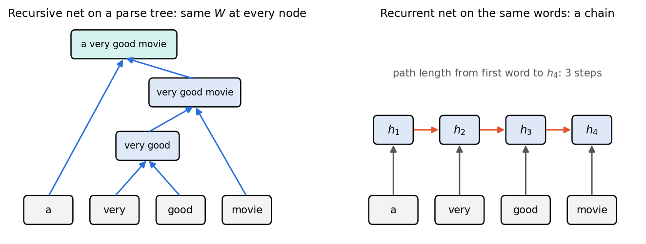
Socher et al. [18] used recursive networks in a vision setting first: they segmented an image into superpixels, then learned both to merge adjacent regions into a scene parse tree and to compute region representations, using the same method to parse sentences. Their later Recursive Neural Tensor Network and Stanford Sentiment Treebank [17] showed that composing along parse trees captures phenomena such as negation (“not very good”). Tai, Socher and Manning’s Tree-LSTM [4] added LSTM-style gates to tree composition, with one forget gate per child, so a parent can selectively keep information from each subtree.
Code · Python · 25 lines
import torch
from torch import nn

torch.manual_seed(0)
D = 8
vocab = {"a": 0, "very": 1, "good": 2, "movie": 3}
emb = nn.Embedding(len(vocab), D)
compose = nn.Linear(2 * D, D)            # ONE weight matrix shared by every internal node
classify = nn.Linear(D, 2)               # e.g. negative / positive sentiment

def encode(tree):
    """tree is a word (leaf) or a pair (left, right)."""
    if isinstance(tree, str):
        return emb(torch.tensor(vocab[tree]))
    left, right = tree
    return torch.tanh(compose(torch.cat([encode(left), encode(right)])))

tree = ("a", (("very", "good"), "movie"))          # (a ((very good) movie))
root = encode(tree)
loss = nn.functional.cross_entropy(classify(root)[None], torch.tensor([1]))
loss.backward()                                     # backpropagation through structure
print("root vector:", tuple(root.shape), "| loss:", round(loss.item(), 4))
print("gradient reached the shared W:", compose.weight.grad.abs().sum().item() > 0)
swapped = encode((("movie", ("good", "very")), "a"))
print("swapping children changes the root:", not torch.allclose(root, swapped))
The recursion is ordinary Python, and autograd builds the tree-shaped graph on the fly. Swapping children changes the result because concatenation gives the left and right slots different roles.
The main practical limitation is the tree itself: someone has to provide it (a parser, a segmentation hierarchy), and batching variable trees efficiently is awkward. Learning structure and representation jointly is possible but harder. In current practice, self-attention can learn soft, input-dependent groupings without an explicit tree, which is one reason recursive networks are now uncommon; the idea of hierarchical composition lives on in hierarchical vision backbones and scene graphs.
Mamba: selective state spaces and scan
A useful memory should hold a relevant observation through distractions and overwrite it when the situation changes. Mamba [21] makes the memory update depend on the current input, while keeping that update affine in the previous state. This distinction lets us retain a recurrent interpretation and compute whole sequences with a parallel prefix scan.
From continuous dynamics to selective updates
Start with a small continuous-time memory. A stable transition lets stored information decay; an input projection writes new information; an output projection reads it:
Here is continuous time, is one input channel, is its -dimensional state, is the transition matrix, writes the input, reads the state, and is the output. A full neural block mixes multiple channels with learned projections and includes additional local convolution and gating [21]. This equation isolates its memory mechanism.
Hold the input and its write matrix constant during each interval. Exact zero-order-hold discretization gives
Here indexes discrete tokens, is the interval length, is an integration variable, is the held input, are the current write/read matrices, and bars mark discrete coefficients. The integral remains valid when is singular; an inverse-based formula needs additional assumptions. A diagonal makes these operations elementwise.
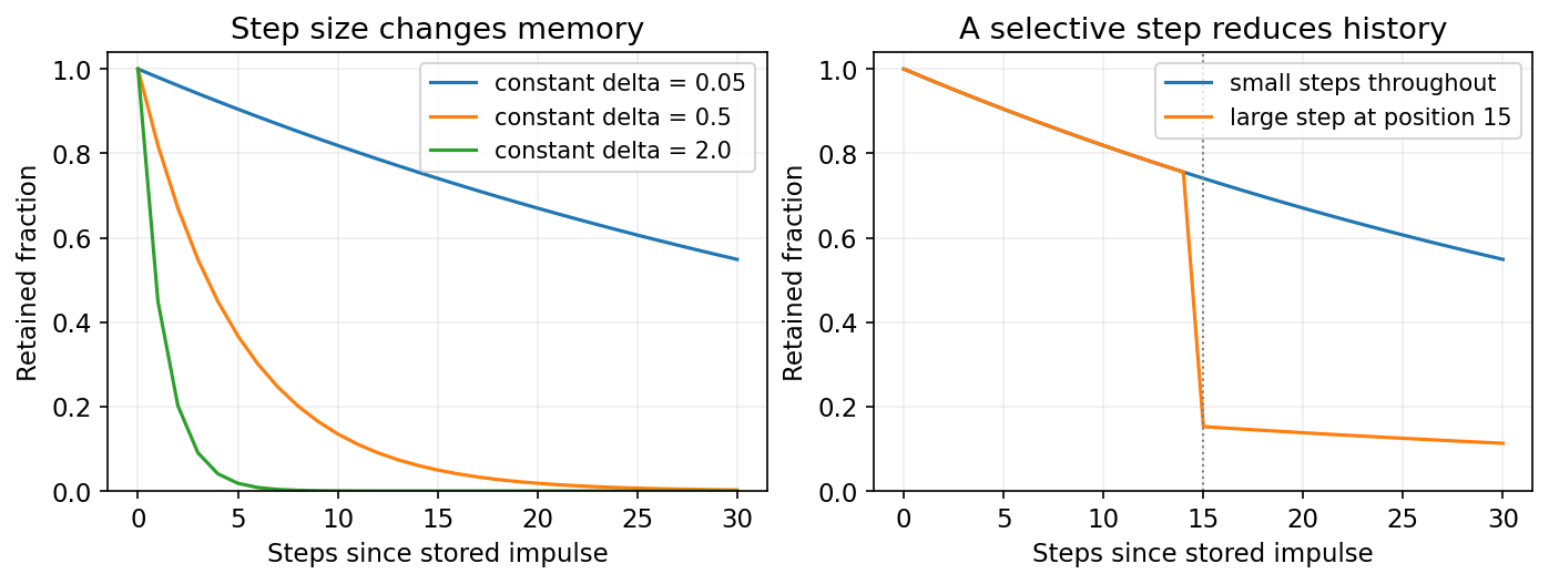
Selectivity means predicting from the current token. For example, a learned affine projection followed by supplies a positive interval. The underlying learned can remain fixed: nevertheless changes through . With negative diagonal entries, a larger interval reduces the fraction of old state retained. Selective writes and reads also determine which content enters and leaves memory. The resulting map is nonlinear in its inputs even though each state update is affine. Figure 7 isolates the retention effect with synthetic coefficients; it does not measure a trained model.
Why this recurrence can be scanned
Once input-dependent coefficients are computed, composing two affine updates requires only another affine update:
Here pair represents , identifies consecutive updates, and means applying the first update and then the second. Composition is associative; for a diagonal transition, products are elementwise. A prefix scan can therefore regroup the operations into a tree while preserving their chronological effect. Ordinary LSTM/GRU gates depend on the previous hidden state, so their coefficients cannot generally be prepared this way before the state is known.
The following standalone CPU example uses exact diagonal discretization and hand-chosen selective coefficients. It checks causality and state continuity across chunks. It is a teaching recurrence, not a pretrained Mamba implementation or a speed benchmark.
Code · Python · 31 lines
import numpy as np

rng = np.random.default_rng(44)
u = rng.normal(size=24)
A = -np.array([0.1, 0.8])  # two stable diagonal entries

def selective_scan(values, state=None):
    h = np.zeros(2) if state is None else state.copy()
    outputs = []
    for x in values:
        delta = np.logaddexp(0.0, 0.5 * x)
        B = np.array([1.0, np.tanh(x)])
        C = np.array([1.0, 0.5 + 0.1 * np.tanh(x)])
        a = np.exp(delta * A)
        b = np.expm1(delta * A) / A * B * x
        h = a * h + b
        outputs.append(C @ h)
    return np.array(outputs), h

y, final_state = selective_scan(u)
changed = u.copy()
changed[12:] += 10.0
changed_y, _ = selective_scan(changed)
assert np.allclose(y[:12], changed_y[:12])
left, boundary = selective_scan(u[:12])
right, resumed_state = selective_scan(u[12:], boundary)
assert np.allclose(y, np.r_[left, right])
assert np.allclose(final_state, resumed_state)
reset_right, _ = selective_scan(u[12:])
assert not np.allclose(right, reset_right)
print('causal prefix and carried-state chunk checks passed')
The output confirms both checks. Resetting the state at a batch boundary changes the computation. Conversely, sharing state between independent examples leaks information. A streaming implementation must track which sequence owns each state and reset it at genuine sequence boundaries.
Mamba-2 and the attention connection
Mamba-2 [29] changes both the inner sequence mixer and the surrounding block. Its structured state-space duality uses a scalar-times-identity transition within each head and organizes computation into chunks whose dense matrix multiplications suit accelerator hardware. It also restructures parameter projections and normalization. This is more specific than adding attention to the original Mamba block.
With a zero initial state, the scalar-transition recurrence can be expanded as
Here indexes earlier inputs, indexes intervening transitions, is the scalar discrete transition multiplying the identity, is the discrete write column, is the read row, and an empty product equals one. The bracketed quantity is a structured causal mixing coefficient. This exposes an attention-like matrix view without requiring ordinary softmax attention or storing that matrix. Hu et al. [30] (ICML 2026) extend the duality to diagonal transitions and clarify why it does not extend directly to standard softmax attention.
At fixed width and state dimension, recurrent inference carries a fixed-size state, whereas ordinary cached causal attention retains keys and values whose storage grows with context length. Compression saves memory but puts pressure on exact recall of many unrelated details. Linear sequence scaling also does not imply constant training memory: activations, gradients and recomputation policies matter. Evaluate retrieval quality, context length and measured device latency together. The image-specific ordering problem appears next in ML 05.
Modern view
Survey literature. Goodfellow et al.’s chapter 10 [1] remains the clearest unified treatment of recurrent and recursive networks, echo-state ideas, and long-term dependencies. Lipton, Berkowitz and Elkan [20] wrote a critical review of RNNs for sequence learning in 2015: a self-contained, historically ordered account of three decades of work leading to LSTMs and bidirectional RNNs, with conflicting notation reconciled and applications to captioning, translation and handwriting recognition. Greff et al. [19] is less a survey than a large empirical study, but it is the reference for which LSTM components matter. Two recent reviews by Tiezzi et al. reframe recurrence for the Transformer era: an extensive survey [26] places Transformer–RNN hybrids, attention variants with recurrent form, and deep state-space models (a special class of linear RNNs) under the single umbrella of recurrence, and highlights research opportunities in learning online from potentially infinite streams rather than fixed-length sequences; and a shorter perspective in Nature Machine Intelligence [27] revisits recurrent processing at the crossroad of Transformers and state-space models.
Recurrence returns (2023–2026). Transformers process all pairs of positions, which costs memory and computation quadratic in length. A family of models revisits recurrence to get linear-time inference with a constant-size state:
- Linear recurrent units. Orvieto et al. [24] (ICML 2023) showed that a carefully parameterized linear recurrence with diagonal complex-valued state matrices, stable initialization and normalization matches deep state-space models on long-range benchmarks, and that the nonlinearity can live outside the recurrence.
- Selective state spaces. Mamba [21] makes the state-space parameters functions of the input, so the model can choose what to store or ignore, as LSTM gates do, while a hardware-aware parallel scan keeps training efficient. Vision variants and the debate about whether they are necessary for images are covered in ML 05.
- Revived LSTMs and GRUs. xLSTM [22] (NeurIPS 2024) adds exponential gating and a matrix-valued memory to the LSTM and scales it to language-model sizes. Feng et al. [23] (2024) remove the hidden-state dependence from the gates of LSTMs and GRUs (“minLSTM”, “minGRU”), which allows a parallel scan during training, and report results competitive with recent sequence models.
The shared lesson is that the gated, additive state update invented for the LSTM was right; what limited classical RNNs was mostly sequential training. Making the recurrence linear in the state (so it can be computed with a parallel scan) recovers parallel training while keeping cheap, streaming inference.
Open problems. Length generalization beyond the training horizon; credit assignment over very long streams without full BPTT; how much a fixed-size state can remember compared with attention’s growing cache, a real limitation for tasks that need exact recall of distant details; and choosing a scan order for 2-D images and 3-D video, where no single natural sequence order exists.
Key takeaways
- An RNN reuses one state-update rule across time; parameter sharing does not guarantee useful long-term memory.
- BPTT sums gradients of shared parameters; truncation limits gradient history while allowing state to continue.
- Clipping limits exploding gradients; additive gated paths help gradient flow without eliminating every long-range learning difficulty.
- Bidirectional encoders use future inputs; causal streaming requires different access and state handling.
- Attention lets a decoder read multiple encoder states; recursive networks instead compose representations along a tree.
- Selective state spaces trade a compact streaming state for compressed history; compare recall and computation under the intended workload.
Exercises
- Causality. Your team reports 92% frame-level accuracy for an action-recognition model with a bidirectional LSTM and proposes deploying it for live alerts. What is wrong with this plan, and how would you evaluate the deployable alternative fairly? Run the selective-scan example, then add a backward scan: which causality check should fail?
Hint
The backward LSTM at frame has read frames after , which a live system has not seen yet. Retrain a unidirectional (causal) model, or allow a fixed look-ahead delay and evaluate with exactly that delay. Report accuracy as a function of latency. A backward scan reads the altered future, so the combined prefix generally changes even when the forward prefix does not.
- Length generalization. Train the GRU sum classifier at length 12, then evaluate on fresh sequences of length 6, 24, 100 and 400 without retraining. Plot accuracy versus length. Then repeat with an LSTM and with training on mixed lengths 6–24.
Hint
Generate fresh data per length. The sum’s scale grows like , so the state may saturate on long inputs even if the logic is right. Mixed-length training usually helps more than switching cell type. Success at length 12 says nothing by itself about length 400.
- Gradient bound. For the scalar RNN , show that . For what values of can the gradient explode, and why does saturation of work against explosion?
Hint
Each factor is with . Explosion requires , but a large also drives toward , which makes small. The gradient explodes only on trajectories that stay in the non-saturated region, which is why explosions are bursty in practice.
- LSTM memory. In the LSTM equations, suppose and for all from to . What is in terms of , and what is along the cell path? What would happen if the forget gate were fixed at 1 forever, as in the original 1997 design, on a never-ending input stream?
Hint
and : perfect memory and perfect gradient flow. With and nonzero writes, the cell state accumulates without bound over an endless stream, which is exactly the problem Gers et al. solved by letting the network learn to forget.
- Attention shapes and masks. In the additive-attention code, a batch has encoder states of shape (with some sequences padded) and a decoder state of shape . Give the shapes of , and the context, and explain what would go wrong if padded positions were masked with instead of .
Hint
and are ; the context is . A score of 0 is an ordinary score: would still give padding positive weight, and the context would mix in meaningless padded states.
- Recursive versus recurrent. For a balanced binary tree over leaves, how many composition steps lie between a leaf and the root? Compare with a left-to-right RNN over the same 1024 inputs, and relate the answer to the vanishing-gradient bound.
Hint
steps versus up to 1023 for the chain. The gradient bound decays like (factor), so a shorter path from each input to the output helps optimization. Attention takes this to the extreme: path length one.
References
- I. Goodfellow, Y. Bengio and A. Courville, Deep Learning, MIT Press, 2016, ch. 10. Book
- S. Hochreiter and J. Schmidhuber, “Long Short-Term Memory,” Neural Computation, 1997. DOI
- K. Cho et al., “Learning Phrase Representations using RNN Encoder–Decoder for Statistical Machine Translation,” EMNLP, 2014. arXiv
- K. S. Tai, R. Socher and C. D. Manning, “Improved Semantic Representations From Tree-Structured Long Short-Term Memory Networks,” ACL, 2015. arXiv
- F. A. Gers, J. Schmidhuber and F. Cummins, “Learning to Forget: Continual Prediction with LSTM,” Neural Computation, 2000. DOI
- Y. Bengio, P. Simard and P. Frasconi, “Learning long-term dependencies with gradient descent is difficult,” IEEE Transactions on Neural Networks, 1994. DOI
- R. Pascanu, T. Mikolov and Y. Bengio, “On the difficulty of training Recurrent Neural Networks,” ICML, 2013. arXiv
- P. J. Werbos, “Backpropagation through time: what it does and how to do it,” Proceedings of the IEEE, 1990. DOI
- J. L. Elman, “Finding Structure in Time,” Cognitive Science, 1990. DOI
- M. Schuster and K. K. Paliwal, “Bidirectional recurrent neural networks,” IEEE Transactions on Signal Processing, 1997. DOI
- I. Sutskever, O. Vinyals and Q. V. Le, “Sequence to Sequence Learning with Neural Networks,” NeurIPS, 2014. arXiv
- D. Bahdanau, K. Cho and Y. Bengio, “Neural Machine Translation by Jointly Learning to Align and Translate,” ICLR, 2015. arXiv
- O. Vinyals, A. Toshev, S. Bengio and D. Erhan, “Show and Tell: A Neural Image Caption Generator,” CVPR, 2015. arXiv
- K. Xu et al., “Show, Attend and Tell: Neural Image Caption Generation with Visual Attention,” ICML, 2015. arXiv
- J. Donahue et al., “Long-term Recurrent Convolutional Networks for Visual Recognition and Description,” CVPR, 2015. arXiv
- X. Shi et al., “Convolutional LSTM Network: A Machine Learning Approach for Precipitation Nowcasting,” NeurIPS, 2015. arXiv
- R. Socher et al., “Recursive Deep Models for Semantic Compositionality Over a Sentiment Treebank,” EMNLP, 2013. Paper
- R. Socher, C. C.-Y. Lin, A. Y. Ng and C. D. Manning, “Parsing Natural Scenes and Natural Language with Recursive Neural Networks,” ICML, 2011. Paper
- K. Greff, R. K. Srivastava, J. Koutník, B. R. Steunebrink and J. Schmidhuber, “LSTM: A Search Space Odyssey,” IEEE Transactions on Neural Networks and Learning Systems, 2017. arXiv
- Z. C. Lipton, J. Berkowitz and C. Elkan, “A Critical Review of Recurrent Neural Networks for Sequence Learning,” arXiv:1506.00019, 2015. arXiv
- A. Gu and T. Dao, “Mamba: Linear-Time Sequence Modeling with Selective State Spaces,” COLM, 2024. arXiv
- M. Beck et al., “xLSTM: Extended Long Short-Term Memory,” NeurIPS, 2024. Paper
- L. Feng et al., “Were RNNs All We Needed?,” arXiv:2410.01201, 2024. arXiv
- A. Orvieto et al., “Resurrecting Recurrent Neural Networks for Long Sequences,” ICML, 2023. arXiv
- S. Bengio, O. Vinyals, N. Jaitly and N. Shazeer, “Scheduled Sampling for Sequence Prediction with Recurrent Neural Networks,” NeurIPS, 2015. arXiv
- M. Tiezzi, M. Casoni, A. Betti, T. Guidi, M. Gori and S. Melacci, “On the Resurgence of Recurrent Models for Long Sequences: Survey and Research Opportunities in the Transformer Era,” arXiv:2402.08132, 2024. arXiv
- M. Tiezzi, M. Casoni, A. Betti, T. Guidi, M. Gori and S. Melacci, “Back to recurrent processing at the crossroad of transformers and state-space models,” Nature Machine Intelligence, 2025. DOI
- A. Vaswani et al., “Attention Is All You Need,” NeurIPS, 2017. arXiv
- T. Dao and A. Gu, “Transformers are SSMs: Generalized Models and Efficient Algorithms Through Structured State Space Duality,” ICML, PMLR 235, 2024. Paper
- J. Y.-C. Hu, X. Zhang, A. Elsheikh, W. Wu and H. Liu, “On Structured State-Space Duality,” ICML, PMLR 306, 2026. Paper
Check your understanding
This tutorial has 6 exercises. Can you solve them without opening the hints?
Go to the exercises ↑Next ML 05 · Attention and Vision Transformers · 25 min