Double descent: reading Belkin, Hsu, Ma and Mandal (PNAS 2019)
Optional · paper guide 1 of 1 for PR 09 · Ensembles, Validation and Cluster Validity. Citation numbers refer to the reference list at the bottom of this page.
Navigate: this page and this track: Navigate: this page and this track
Plain version. The textbook picture says that a model with more freedom than it needs will memorize the noise and do worse on new data. This paper asks what happens if you keep adding freedom long after the model already fits the training set exactly. Its answer: the test error can first shoot up and then come back down, so the curve has two descents instead of one valley.
Challenge
Large neural networks are routinely trained until the training error is (nearly) zero, yet they predict well. A reader who has just met the bias–variance decomposition would call that overfitting. Belkin and colleagues [25] ask whether the classical U-shaped risk curve and this practice can be one picture.
Method
They draw a single curve of test risk against model capacity with two regimes separated by the interpolation threshold, the capacity at which the model class can first fit the training set exactly. Left of it is the classical U. Right of it, every model has zero training error, and the claim is that test risk typically falls again as capacity grows. Their posited mechanism is an inductive bias: among all interpolating functions, a bigger class contains smoother ones (smaller norm), and the training procedure finds a small-norm one. For random features this is explicit. With the matrix of feature values at training points, the labels and the Moore–Penrose pseudo-inverse, the learned coefficients are
the interpolating solution with the smallest norm when the constraint is feasible. Full row rank of guarantees feasibility for every ; merely having does not. If duplicate or dependent features make rank deficient and is outside its column space, is instead the minimum-norm least-squares solution and need not interpolate [27]. Count effective rank as well as parameters when locating an interpolation threshold.
Results
Read the setup carefully, because “capacity” is not one thing across the figures.
- Random Fourier features (RFF), MNIST. Capacity is the number of random Fourier features , with a subset of MNIST images and 10 classes; the interpolation threshold is at , and the plotted range runs to (their Figure 2). Each model is fit by least squares on the squared loss, taking the minimum--norm coefficients when . Test risk is shown for both zero-one loss and squared loss, next to the coefficient norm and the training risk. The paper reports that at the predictor has no predictive ability for classification, and that for larger accuracy improves beyond the bottom of the U. RFF results come from a single run, which the authors describe as highly consistent.
- Two-layer fully connected network, MNIST. Capacity is the number of weights, for hidden units, input dimension and outputs, trained on images; the threshold is observed at (their Figure 4). Training uses SGD; below the threshold the smaller network’s weights initialize the larger one (“weight reuse”), and the paper notes that without it the variance is much larger but double descent is still visible. Network and ensemble results are means over five runs.
- Random forests. Capacity is a hybrid index: the number of leaves per tree up to the point where trees interpolate, then the number of averaged interpolating trees beyond it (their Figure 5). The x-axis here is stitched from two different knobs.
- A synthetic model with a known target and noise, averaged over 20 trials, where the peak sits at (their Appendix C.4).
Reading the evidence
Look at their Figure 2 first. Then check: (1) which loss: squared loss was optimized, zero-one loss is what you care about for classification, and both are shown; (2) which axis: the same word “capacity” means features, weights or trees, so a peak “at the threshold” depends on the counting rule; (3) which solution: the second descent is for the minimum-norm interpolator, not for any interpolator; (4) noise: the text describes no label corruption in the MNIST experiments, and noise appears only in the synthetic model, so the paper does not show how the MNIST curves change as noise is added; (5) how many runs: one for RFF, five for networks and ensembles, 20 for the synthetic model, and the paper’s own caution that a single bad initialization of a network can hide the shape; (6) log axes: the squared-loss panel is on a log scale, which makes a narrow peak look dramatic.
Problems
The paper itself says that for ImageNet-scale problems interpolation might need on the order of parameters, larger than many networks used there, so such models would sit in the classical regime. It also notes that regularization and early stopping can prevent interpolation and hide the peak, and that the mechanism is “posited”: the precise statement it proves is for noiseless data. The experiments use subsets of standard datasets, and the single-run RFF curves carry no information about repeat-to-repeat spread.
Conclusion
The bias–variance decomposition earlier in this tutorial is exact; what the paper changes is the common reading of it as “more capacity means more variance”. The same lesson applies to validation: a model-selection sweep that stops just past the peak, or that uses early stopping, only sees the left half of the picture.
Worked experiment
The script below fits 1-D regression with random Fourier-type features and training points, using numpy.linalg.lstsq, which returns the minimum-norm solution when . Feature is a cosine or sine of integer frequency, with weight ; the target is plus Gaussian label noise at signal-to-noise ratio 20, and the columns are scaled by so that the plain norm is a smoothness-weighted norm, in the spirit of the paper’s synthetic model. Test MSE is measured against the noiseless target (add for the risk on noisy labels), as the median of 50 repeats.
Code · Python · 34 lines
import numpy as np

n, K, snr, n_rep = 40, 2000, 20.0, 50           # training size, feature pool, signal-to-noise ratio, repeats
counts = [1, 3, 8, 20, 30, 38, 40, 42, 50, 80, 200, 1000, 2000]   # numbers of features N
k = np.arange(K)
p = 1.0 / (k + 1) ** 1.5
p /= p.sum()                                    # weight p_k of feature k (low frequencies matter most)
freq = (k + 1) // 2                             # feature k: cos or sin of (freq * x)

def basis(x, idx):
    arg = np.outer(x, freq[idx])
    return np.where(idx % 2 == 0, np.cos(arg), np.sin(arg))

x_test = np.linspace(0, 2 * np.pi, 1000, endpoint=False)
h_test = basis(x_test, k) @ p                   # noiseless target h*(x) = sum_k p_k e_k(x)
sigma = np.sqrt(np.mean(h_test ** 2) / snr)     # label-noise level implied by the SNR

def one_run(rng):
    x = rng.uniform(0, 2 * np.pi, n)
    y = basis(x, k) @ p + sigma * rng.standard_normal(n)
    order = rng.choice(K, size=max(counts), replace=False, p=p)   # nested random feature sets
    out = []
    for N in counts:
        idx = order[:N]
        A = basis(x, idx) * np.sqrt(p[idx])     # rescale columns so the plain l2 norm is the weighted norm
        beta = np.linalg.lstsq(A, y, rcond=None)[0]   # least squares; minimum-norm solution when N > n
        pred = basis(x_test, idx) @ (beta * np.sqrt(p[idx]))
        out.append((np.mean((pred - h_test) ** 2), np.mean((A @ beta - y) ** 2)))
    return out

res = np.array([one_run(np.random.default_rng(s)) for s in range(n_rep)])   # shape (repeat, N, [test, train])
print(f"label-noise variance sigma^2 = {sigma**2:.4f}")
for N, te, tr in zip(counts, np.median(res[:, :, 0], 0), np.median(res[:, :, 1], 0)):
    print(f"N = {N:4d}   train MSE {tr:.2e}   test MSE {te:.2e}")
On our run:
Code · 14 lines
label-noise variance sigma^2 = 0.0084
N =    1   train MSE 1.51e-01   test MSE 1.63e-01
N =    3   train MSE 1.93e-02   test MSE 1.56e-02
N =    8   train MSE 8.13e-03   test MSE 5.80e-03
N =   20   train MSE 3.90e-03   test MSE 1.08e-02
N =   30   train MSE 1.72e-03   test MSE 2.81e-02
N =   38   train MSE 2.26e-04   test MSE 4.29e-01
N =   40   train MSE 6.22e-29   test MSE 4.62e+00
N =   42   train MSE 6.99e-30   test MSE 9.43e-01
N =   50   train MSE 3.30e-30   test MSE 2.50e-01
N =   80   train MSE 2.89e-30   test MSE 4.07e-02
N =  200   train MSE 1.34e-30   test MSE 9.39e-03
N = 1000   train MSE 2.20e-30   test MSE 4.00e-03
N = 2000   train MSE 2.01e-30   test MSE 3.71e-03
The training MSE drops to numerical zero exactly at . The test MSE has a classical valley (lowest among these counts, at ), explodes to at , about 800 times the valley, and then falls steadily to at , somewhat below the valley. Figure S1 shows the same experiment on a denser grid of .
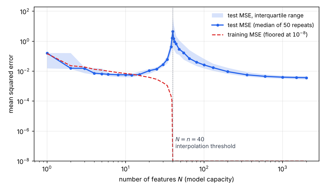
Two cautions about this toy. The second descent only reaches the valley’s level here because the weighting matches how the target was built; in a trial run with a steeper decay of the weights (exponent 2 instead of 1.5), the right-hand end stayed above the bottom of the U. That is the paper’s point in miniature: the benefit comes from the norm bias matching the problem, not from size as such. And the median hides a heavy tail: at the 50 repeats range from to (median , mean ), because a few random feature draws are extremely ill-conditioned, so a mean over repeats would be dominated by the worst draws.
Common misinterpretation
Reading “double descent” as “bigger is always better”, or as a statement about all models. It describes interpolating, minimum-norm-like solutions in a particular range of capacity; regularized models, early-stopped networks and models far below the threshold follow the classical rules.
References
-
S. Theodoridis and K. Koutroumbas, Pattern Recognition, 4th ed., Academic Press, 2009. Chapter 4 (decision trees, combining classifiers, boosting), Chapter 10 (“Supervised Learning: The Epilogue”) and Chapter 16 (“Cluster Validity”). doi
-
C. M. Bishop, Pattern Recognition and Machine Learning, Springer, 2006. Sections 1.3 and 3.2 (model selection, bias–variance) and 14.1–14.5 (Bayesian model averaging, committees, boosting, trees, conditional mixtures). official book and PDF
-
S. Geman, E. Bienenstock and R. Doursat, “Neural networks and the bias/variance dilemma,” Neural Computation, vol. 4, no. 1, pp. 1–58, 1992. doi
-
L. Breiman, “Bagging predictors,” Machine Learning, vol. 24, no. 2, pp. 123–140, 1996. doi
-
L. Breiman, “Random forests,” Machine Learning, vol. 45, no. 1, pp. 5–32, 2001. doi
-
Y. Freund and R. E. Schapire, “A decision-theoretic generalization of on-line learning and an application to boosting,” Journal of Computer and System Sciences, vol. 55, no. 1, pp. 119–139, 1997. doi
-
J. Friedman, T. Hastie and R. Tibshirani, “Additive logistic regression: A statistical view of boosting (with discussion),” The Annals of Statistics, vol. 28, no. 2, 2000. doi
-
J. H. Friedman, “Greedy function approximation: A gradient boosting machine,” The Annals of Statistics, vol. 29, no. 5, 2001. doi
-
T. Chen and C. Guestrin, “XGBoost: A scalable tree boosting system,” in Proc. 22nd ACM SIGKDD International Conference on Knowledge Discovery and Data Mining, pp. 785–794, 2016. doi
-
D. H. Wolpert, “Stacked generalization,” Neural Networks, vol. 5, no. 2, pp. 241–259, 1992. doi
-
B. Efron and R. Tibshirani, “Improvements on cross-validation: The .632+ bootstrap method,” Journal of the American Statistical Association, vol. 92, no. 438, pp. 548–560, 1997. doi
-
S. Varma and R. Simon, “Bias in error estimation when using cross-validation for model selection,” BMC Bioinformatics, vol. 7, 91, 2006. doi
-
G. C. Cawley and N. L. C. Talbot, “On over-fitting in model selection and subsequent selection bias in performance evaluation,” Journal of Machine Learning Research, vol. 11, pp. 2079–2107, 2010. JMLR
-
T. G. Dietterich, “Approximate statistical tests for comparing supervised classification learning algorithms,” Neural Computation, vol. 10, no. 7, pp. 1895–1923, 1998. doi
-
C. Nadeau and Y. Bengio, “Inference for the generalization error,” Machine Learning, vol. 52, no. 3, pp. 239–281, 2003. doi
-
J. Demšar, “Statistical comparisons of classifiers over multiple data sets,” Journal of Machine Learning Research, vol. 7, pp. 1–30, 2006. JMLR
-
A. Benavoli, G. Corani, J. Demšar and M. Zaffalon, “Time for a change: A tutorial for comparing multiple classifiers through Bayesian analysis,” Journal of Machine Learning Research, vol. 18, no. 77, pp. 1–36, 2017. JMLR
-
S. Arlot and A. Celisse, “A survey of cross-validation procedures for model selection,” Statistics Surveys, vol. 4, pp. 40–79, 2010. doi
-
S. Bates, T. Hastie and R. Tibshirani, “Cross-validation: What does it estimate and how well does it do it?,” Journal of the American Statistical Association, vol. 119, no. 546, pp. 1434–1445, 2024. doi
-
S. Raschka, “Model evaluation, model selection, and algorithm selection in machine learning,” arXiv:1811.12808, 2018. arXiv
-
X. Dong, Z. Yu, W. Cao, Y. Shi and Q. Ma, “A survey on ensemble learning,” Frontiers of Computer Science, vol. 14, no. 2, pp. 241–258, 2020. doi
-
M. A. Ganaie, M. Hu, A. K. Malik, M. Tanveer and P. N. Suganthan, “Ensemble deep learning: A review,” Engineering Applications of Artificial Intelligence, vol. 115, 105151, 2022. doi
-
L. Grinsztajn, E. Oyallon and G. Varoquaux, “Why do tree-based models still outperform deep learning on typical tabular data?,” in Advances in Neural Information Processing Systems (NeurIPS) Datasets and Benchmarks Track, 2022 (arXiv:2207.08815). arXiv
-
B. Lakshminarayanan, A. Pritzel and C. Blundell, “Simple and scalable predictive uncertainty estimation using deep ensembles,” in Advances in Neural Information Processing Systems (NIPS), 2017 (arXiv:1612.01474). arXiv
-
M. Belkin, D. Hsu, S. Ma and S. Mandal, “Reconciling modern machine-learning practice and the classical bias–variance trade-off,” Proceedings of the National Academy of Sciences, vol. 116, no. 32, pp. 15849–15854, 2019. doi
-
scikit-learn developers, scikit-learn User Guide: ensemble methods, cross-validation, probability calibration and clustering performance evaluation.
-
NumPy developers, “numpy.linalg.lstsq,” API documentation, accessed 2026-11-05. documentation