雙重下降:Belkin 等人(PNAS 2019)閱讀指南
選讀・PR 09・集成、驗證與分群有效性 的論文導讀(第 1/1 篇)。引用編號對應本頁底部的參考文獻。
導覽:本頁與本系列: 導覽:本頁與本系列
白話版。 教科書的圖像說:模型的自由度若超過所需,就會把雜訊也背下來,對新資料表現更差。這篇論文問的是:如果在模型早已完全擬合訓練集之後,還繼續增加自由度,會發生什麼事?它的答案是:測試誤差可能先飆高、再降下來,所以曲線不是一個山谷,而是兩次下降。
挑戰
大型神經網路常被訓練到訓練誤差(幾乎)為零,卻仍能做出良好預測。剛學過偏差–變異數分解的讀者會把這稱為過擬合。Belkin 等人 [25] 想知道:經典的 U 形風險曲線與這種實務做法,能不能放進同一張圖。
方法
他們畫出一條測試風險對模型容量(capacity)的曲線,分成兩個區段,以內插門檻(interpolation threshold)為界,也就是模型類別第一次能完全擬合訓練集的容量。門檻左邊是經典的 U 形;右邊每個模型的訓練誤差都是零,而論文的主張是:容量繼續增加時,測試風險通常會再次下降。他們提出的機制是一種歸納偏好(inductive bias):在所有能內插資料的函數中,較大的類別含有較平滑(範數較小)的函數,而訓練程序會找到範數小的那一個。對隨機特徵而言這是明確的:令 為 個特徵在 個訓練點上的取值矩陣, 為標籤, 為 Moore–Penrose 偽逆矩陣(pseudo-inverse),則學到的係數為
這是在約束可行時,所有內插解中 範數最小的解。 滿列秩(full row rank)才能保證任意 都可行,只有 並不足夠。若重複或相依特徵使 秩不足,且 不在其欄空間中, 就只是最小範數的最小平方解,不一定能內插 [27]。尋找內插門檻時,應同時看有效秩與參數數量。
結果
請仔細讀實驗設定,因為「容量」在各張圖中並不是同一件事。
- 隨機傅立葉特徵(random Fourier features, RFF),MNIST。 容量是隨機傅立葉特徵的數量 ,使用 張 MNIST 影像的子集與 10 個類別;內插門檻在 ,繪圖範圍延伸到 (論文圖 2)。每個模型用平方損失做最小平方法擬合,當 時取 範數最小的係數。測試風險同時以 0–1 損失與平方損失呈現,並與係數範數和訓練風險並列。論文報告:在 時,預測器對分類毫無預測能力; 更大時,準確率改善到超過 U 形谷底。RFF 的結果來自單次執行,作者說這些結果高度一致。
- 兩層全連接網路,MNIST。 容量是權重數量, 個隱藏單元時為 ,其中輸入維度 、輸出數 ,在 張影像上訓練;門檻出現在 (論文圖 4)。訓練使用 SGD;門檻以下以較小網路的權重初始化較大的網路(「權重重用」,weight reuse),論文指出沒有權重重用時變異大得多,但雙重下降仍然看得出來。網路與整體法的結果是五次執行的平均。
- 隨機森林。 容量是混合式的索引:到樹能完全內插為止,用每棵樹的葉節點數;超過之後,用被平均的內插樹的棵數(論文圖 5)。這裡的橫軸是由兩種不同的旋鈕接起來的。
- 一個合成模型,目標函數與雜訊皆已知,平均 20 次試驗,峰值出現在 (論文附錄 C.4)。
判讀證據
先看論文的圖 2。接著檢查:(1)哪種損失:最佳化的是平方損失,分類真正在意的是 0–1 損失,兩者都有呈現;(2)哪條軸:同樣叫「容量」,可以是特徵數、權重數或樹的棵數,所以「峰值在門檻」取決於計數規則;(3)哪個解:第二次下降屬於最小範數的內插解,而不是任意內插解;(4)雜訊:文中描述的 MNIST 實驗沒有加入標籤污染,雜訊只出現在合成模型,所以論文並未顯示 MNIST 曲線在加入雜訊後如何變化;(5)執行幾次:RFF 一次、網路與整體法五次、合成模型 20 次,而且論文自己也提醒,單次不佳的網路初始化可能掩蓋曲線的形狀;(6)對數軸:平方損失那一欄用對數刻度,會讓狹窄的峰顯得很誇張。
限制與問題
論文自己指出,對 ImageNet 規模的問題,內插可能需要約 個參數,比那裡使用的許多網路都大,因此這類模型落在經典區段。它也提到正則化與提早停止可能使模型無法內插、並掩蓋峰值,而且機制只是「提出的假說」:嚴格證明的陳述針對的是無雜訊資料。實驗使用標準資料集的子集,單次執行的 RFF 曲線也看不出重複之間的波動。
結論
本章前面的偏差–變異數分解是精確的;這篇論文改變的是人們常把它讀成「容量越大、變異數越大」的那種讀法。同樣的教訓也適用於驗證:模型選擇的掃描若停在峰值剛過的地方,或使用提早停止,就只看得到圖的左半邊。
實作範例
下面的程式以 個隨機傅立葉型特徵與 個訓練點擬合一維迴歸,使用 numpy.linalg.lstsq;當 時,它回傳最小範數解。第 個特徵是整數頻率的餘弦或正弦,權重為 ;目標函數為 加上訊雜比為 20 的高斯標籤雜訊,並把各欄乘上 ,使一般的 範數成為依平滑度加權的範數,這與論文的合成模型精神相同。測試 MSE 是相對於無雜訊目標計算的(若要得到含雜訊標籤的風險,請再加 ),取 50 次重複的中位數。
程式碼 · Python · 34 行
import numpy as np

n, K, snr, n_rep = 40, 2000, 20.0, 50           # training size, feature pool, signal-to-noise ratio, repeats
counts = [1, 3, 8, 20, 30, 38, 40, 42, 50, 80, 200, 1000, 2000]   # numbers of features N
k = np.arange(K)
p = 1.0 / (k + 1) ** 1.5
p /= p.sum()                                    # weight p_k of feature k (low frequencies matter most)
freq = (k + 1) // 2                             # feature k: cos or sin of (freq * x)

def basis(x, idx):
    arg = np.outer(x, freq[idx])
    return np.where(idx % 2 == 0, np.cos(arg), np.sin(arg))

x_test = np.linspace(0, 2 * np.pi, 1000, endpoint=False)
h_test = basis(x_test, k) @ p                   # noiseless target h*(x) = sum_k p_k e_k(x)
sigma = np.sqrt(np.mean(h_test ** 2) / snr)     # label-noise level implied by the SNR

def one_run(rng):
    x = rng.uniform(0, 2 * np.pi, n)
    y = basis(x, k) @ p + sigma * rng.standard_normal(n)
    order = rng.choice(K, size=max(counts), replace=False, p=p)   # nested random feature sets
    out = []
    for N in counts:
        idx = order[:N]
        A = basis(x, idx) * np.sqrt(p[idx])     # rescale columns so the plain l2 norm is the weighted norm
        beta = np.linalg.lstsq(A, y, rcond=None)[0]   # least squares; minimum-norm solution when N > n
        pred = basis(x_test, idx) @ (beta * np.sqrt(p[idx]))
        out.append((np.mean((pred - h_test) ** 2), np.mean((A @ beta - y) ** 2)))
    return out

res = np.array([one_run(np.random.default_rng(s)) for s in range(n_rep)])   # shape (repeat, N, [test, train])
print(f"label-noise variance sigma^2 = {sigma**2:.4f}")
for N, te, tr in zip(counts, np.median(res[:, :, 0], 0), np.median(res[:, :, 1], 0)):
    print(f"N = {N:4d}   train MSE {tr:.2e}   test MSE {te:.2e}")
在我們的執行中:
程式碼 · 14 行
label-noise variance sigma^2 = 0.0084
N =    1   train MSE 1.51e-01   test MSE 1.63e-01
N =    3   train MSE 1.93e-02   test MSE 1.56e-02
N =    8   train MSE 8.13e-03   test MSE 5.80e-03
N =   20   train MSE 3.90e-03   test MSE 1.08e-02
N =   30   train MSE 1.72e-03   test MSE 2.81e-02
N =   38   train MSE 2.26e-04   test MSE 4.29e-01
N =   40   train MSE 6.22e-29   test MSE 4.62e+00
N =   42   train MSE 6.99e-30   test MSE 9.43e-01
N =   50   train MSE 3.30e-30   test MSE 2.50e-01
N =   80   train MSE 2.89e-30   test MSE 4.07e-02
N =  200   train MSE 1.34e-30   test MSE 9.39e-03
N = 1000   train MSE 2.20e-30   test MSE 4.00e-03
N = 2000   train MSE 2.01e-30   test MSE 3.71e-03
訓練 MSE 恰在 時掉到數值上的零。測試 MSE 先有一個經典的谷底(在這些特徵數中最低, 時為 ),到 時暴增到 ,約為谷底的 800 倍,之後穩定下降,在 時為 ,略低於谷底。圖 S1 以更密的 網格呈現同一個實驗。
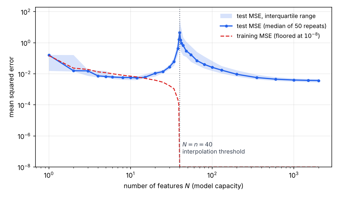
關於這個玩具實驗有兩點提醒。第二次下降只在這裡回到谷底的水準,是因為權重 與目標函數的建構方式相吻合;在試跑中改用較陡的權重衰減(指數 2 而非 1.5)時,右端仍然高於 U 形谷底。這正是論文要點的縮影:好處來自範數偏好與問題相符,而不是來自規模本身。另外,中位數掩蓋了重尾:在 時,50 次重複的範圍從 到 (中位數 ,平均 ),因為少數隨機特徵抽樣的條件數極差,所以對重複取平均會被最糟的幾次主導。
常見誤讀
把「雙重下降」讀成「越大越好」,或當成對所有模型都成立的陳述。它描述的是在某段容量範圍內、能內插資料的最小範數類型解;經過正則化的模型、提早停止的網路,以及遠低於門檻的模型,仍然遵循經典規則。
參考文獻
-
S. Theodoridis and K. Koutroumbas, Pattern Recognition, 4th ed., Academic Press, 2009. 第 4 章(決策樹、分類器組合、boosting)、第 10 章(「Supervised Learning: The Epilogue」)與第 16 章(「Cluster Validity」)。doi
-
C. M. Bishop, Pattern Recognition and Machine Learning, Springer, 2006. 第 1.3 與 3.2 節(模型選擇、偏差–變異數)及第 14.1–14.5 節(貝氏模型平均、委員會、boosting、樹、條件式混合)。官方書籍與 PDF
-
S. Geman, E. Bienenstock and R. Doursat, “Neural networks and the bias/variance dilemma,” Neural Computation, vol. 4, no. 1, pp. 1–58, 1992. doi
-
L. Breiman, “Bagging predictors,” Machine Learning, vol. 24, no. 2, pp. 123–140, 1996. doi
-
L. Breiman, “Random forests,” Machine Learning, vol. 45, no. 1, pp. 5–32, 2001. doi
-
Y. Freund and R. E. Schapire, “A decision-theoretic generalization of on-line learning and an application to boosting,” Journal of Computer and System Sciences, vol. 55, no. 1, pp. 119–139, 1997. doi
-
J. Friedman, T. Hastie and R. Tibshirani, “Additive logistic regression: A statistical view of boosting (with discussion),” The Annals of Statistics, vol. 28, no. 2, 2000. doi
-
J. H. Friedman, “Greedy function approximation: A gradient boosting machine,” The Annals of Statistics, vol. 29, no. 5, 2001. doi
-
T. Chen and C. Guestrin, “XGBoost: A scalable tree boosting system,” in Proc. 22nd ACM SIGKDD International Conference on Knowledge Discovery and Data Mining, pp. 785–794, 2016. doi
-
D. H. Wolpert, “Stacked generalization,” Neural Networks, vol. 5, no. 2, pp. 241–259, 1992. doi
-
B. Efron and R. Tibshirani, “Improvements on cross-validation: The .632+ bootstrap method,” Journal of the American Statistical Association, vol. 92, no. 438, pp. 548–560, 1997. doi
-
S. Varma and R. Simon, “Bias in error estimation when using cross-validation for model selection,” BMC Bioinformatics, vol. 7, 91, 2006. doi
-
G. C. Cawley and N. L. C. Talbot, “On over-fitting in model selection and subsequent selection bias in performance evaluation,” Journal of Machine Learning Research, vol. 11, pp. 2079–2107, 2010. JMLR
-
T. G. Dietterich, “Approximate statistical tests for comparing supervised classification learning algorithms,” Neural Computation, vol. 10, no. 7, pp. 1895–1923, 1998. doi
-
C. Nadeau and Y. Bengio, “Inference for the generalization error,” Machine Learning, vol. 52, no. 3, pp. 239–281, 2003. doi
-
J. Demšar, “Statistical comparisons of classifiers over multiple data sets,” Journal of Machine Learning Research, vol. 7, pp. 1–30, 2006. JMLR
-
A. Benavoli, G. Corani, J. Demšar and M. Zaffalon, “Time for a change: A tutorial for comparing multiple classifiers through Bayesian analysis,” Journal of Machine Learning Research, vol. 18, no. 77, pp. 1–36, 2017. JMLR
-
S. Arlot and A. Celisse, “A survey of cross-validation procedures for model selection,” Statistics Surveys, vol. 4, pp. 40–79, 2010. doi
-
S. Bates, T. Hastie and R. Tibshirani, “Cross-validation: What does it estimate and how well does it do it?,” Journal of the American Statistical Association, vol. 119, no. 546, pp. 1434–1445, 2024. doi
-
S. Raschka, “Model evaluation, model selection, and algorithm selection in machine learning,” arXiv:1811.12808, 2018. arXiv
-
X. Dong, Z. Yu, W. Cao, Y. Shi and Q. Ma, “A survey on ensemble learning,” Frontiers of Computer Science, vol. 14, no. 2, pp. 241–258, 2020. doi
-
M. A. Ganaie, M. Hu, A. K. Malik, M. Tanveer and P. N. Suganthan, “Ensemble deep learning: A review,” Engineering Applications of Artificial Intelligence, vol. 115, 105151, 2022. doi
-
L. Grinsztajn, E. Oyallon and G. Varoquaux, “Why do tree-based models still outperform deep learning on typical tabular data?,” in Advances in Neural Information Processing Systems (NeurIPS) Datasets and Benchmarks Track, 2022 (arXiv:2207.08815). arXiv
-
B. Lakshminarayanan, A. Pritzel and C. Blundell, “Simple and scalable predictive uncertainty estimation using deep ensembles,” in Advances in Neural Information Processing Systems (NIPS), 2017 (arXiv:1612.01474). arXiv
-
M. Belkin, D. Hsu, S. Ma and S. Mandal, “Reconciling modern machine-learning practice and the classical bias–variance trade-off,” Proceedings of the National Academy of Sciences, vol. 116, no. 32, pp. 15849–15854, 2019. doi
-
scikit-learn developers, scikit-learn User Guide:集成方法、交叉驗證、機率校準與分群效能評估。
-
NumPy developers, “numpy.linalg.lstsq,” API documentation, accessed 2026-11-05. documentation