Probabilistic PCA — a density model behind a subspace
Optional · paper guide 1 of 1 for ML 06A · Linear Factor Models and Autoencoders. Citation numbers refer to the reference list at the bottom of this page.
Navigate: this page and this track: Navigate: this page and this track
Question and thesis
Can PCA be expressed as a probabilistic generative model rather than only a geometric projection? Tipping and Bishop show how a Gaussian latent-variable model recovers the principal subspace while providing a likelihood and a route for inference with missing observations [4]. Start with eigenvectors, covariance and Gaussian distributions. This paper supplies a bridge from ML 01A’s geometry to the latent-variable models in this chapter.
Method and figure
The model assumes
Here is the observed vector, is a lower-dimensional latent vector, is a loading matrix, is the data mean, is independent isotropic noise, and is its variance. Each identity matrix has the dimension of the corresponding space. Integrating out gives the displayed observation distribution.
Maximum likelihood aligns the learned loading subspace with leading covariance eigenvectors. Latent coordinates are not uniquely identified: rotations can preserve the observation distribution. At finite noise, a posterior latent mean is also not simply the ordinary orthogonal PCA projection. Keep the subspace, loading parameters and inferred coordinates conceptually separate.
Evidence
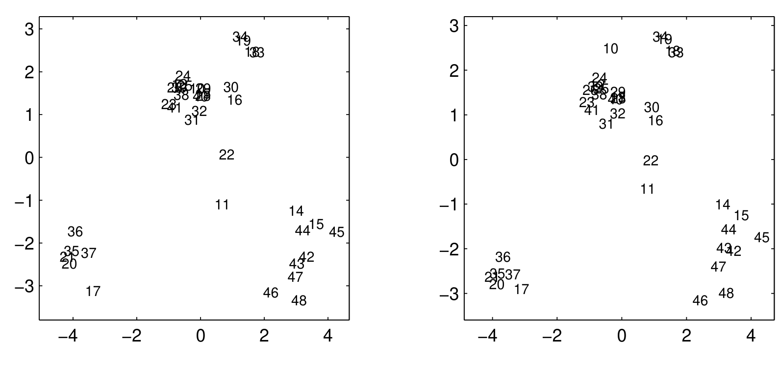
The central evidence includes a likelihood derivation and an expectation-maximization procedure, not a new neural architecture benchmark. Figure 1 illustrates missing-data inference using 38 observations with 18 dimensions. Values are removed independently with probability 20%; the shown case has 136 missing values. The inferred projection retains recognizable groups and the highlighted outlier. This supports the illustrated use case, not universal robustness to arbitrary missingness.
Design analysis
A probability model makes conditional inference possible using the coordinates that were actually observed. It also exposes assumptions that ordinary projection notation can hide: linear structure, Gaussian latent variables and equal noise variance in every observation direction. The missing-data example tests one practical consequence of the model. It does not demonstrate that the observation mechanism itself is correctly modeled when values are missing for informative reasons.
Reading checkpoint
Explain why changing the orientation of latent axes need not change the modeled observation density. Then consider an observation with one missing coordinate: which observed entries should condition the prediction, and why is replacing the missing value with zero generally a different procedure?
Limits and next step
A single linear Gaussian component cannot represent every curved or multimodal distribution. Its likelihood is useful only to the extent that its assumptions fit the task. Next read the VAE guide in ML 07: compare the linear decoder and tractable posterior here with a nonlinear decoder and learned approximate posterior there.
Continue reading: VAE — learning through a tractable lower bound
References
- I. Goodfellow, Y. Bengio and A. Courville, Deep Learning, MIT Press, 2016, ch. 13–14. Book
- K. P. Murphy, Probabilistic Machine Learning: An Introduction, MIT Press, 2022. Book
- Y. Bengio, A. Courville and P. Vincent, “Representation Learning: A Review and New Perspectives,” IEEE Transactions on Pattern Analysis and Machine Intelligence, vol. 35, no. 8, 2013. Paper
- M. E. Tipping and C. M. Bishop, “Probabilistic Principal Component Analysis,” Journal of the Royal Statistical Society: Series B, vol. 61, no. 3, 1999. Paper
- A. Hyvärinen and E. Oja, “Independent component analysis: algorithms and applications,” Neural Networks, vol. 13, no. 4–5, 2000. Paper
- B. A. Olshausen and D. J. Field, “Emergence of simple-cell receptive field properties by learning a sparse code for natural images,” Nature, vol. 381, 1996. Paper
- D. D. Lee and H. S. Seung, “Learning the parts of objects by non-negative matrix factorization,” Nature, vol. 401, 1999. Paper
- P. Baldi and K. Hornik, “Neural networks and principal component analysis: Learning from examples without local minima,” Neural Networks, vol. 2, no. 1, 1989. Paper
- G. E. Hinton and R. R. Salakhutdinov, “Reducing the Dimensionality of Data with Neural Networks,” Science, vol. 313, 2006. Paper
- P. Vincent, H. Larochelle, Y. Bengio and P.-A. Manzagol, “Extracting and composing robust features with denoising autoencoders,” ICML, 2008. Paper
- P. Vincent, H. Larochelle, I. Lajoie, Y. Bengio and P.-A. Manzagol, “Stacked Denoising Autoencoders: Learning Useful Representations in a Deep Network with a Local Denoising Criterion,” JMLR, vol. 11, 2010. Paper
- S. Rifai, P. Vincent, X. Muller, X. Glorot and Y. Bengio, “Contractive Auto-Encoders: Explicit Invariance During Feature Extraction,” ICML, 2011. Paper
- D. P. Kingma and M. Welling, “Auto-Encoding Variational Bayes,” ICLR, 2014. Paper
- D. P. Kingma and M. Welling, “An Introduction to Variational Autoencoders,” Foundations and Trends in Machine Learning, vol. 12, no. 4, 2019. Paper
- I. Higgins et al., “β-VAE: Learning Basic Visual Concepts with a Constrained Variational Framework,” ICLR, 2017. Paper
- D. Bank, N. Koenigstein and R. Giryes, “Autoencoders,” survey chapter, arXiv:2003.05991, 2020. Survey
- F. Locatello et al., “Challenging Common Assumptions in the Unsupervised Learning of Disentangled Representations,” ICML, 2019. Paper
- A. van den Oord, O. Vinyals and K. Kavukcuoglu, “Neural Discrete Representation Learning,” NeurIPS, 2017. Paper
- R. Rombach, A. Blattmann, D. Lorenz, P. Esser and B. Ommer, “High-Resolution Image Synthesis with Latent Diffusion Models,” CVPR, 2022. Paper
- H. Cunningham, A. Ewart, L. Riggs, R. Huben and L. Sharkey, “Sparse Autoencoders Find Highly Interpretable Features in Language Models,” arXiv:2309.08600, 2023. Paper
- L. Gao et al., “Scaling and evaluating sparse autoencoders,” arXiv:2406.04093, 2024. Paper