DLCV 13 · World Models: Video, Latent Dynamics and Planning
Needs: ML 04 · Recurrent and Recursive Networks, ML 10 · Foundation Models and Vision–Language Learning, DLCV 07 · Object Tracking: From Single-Object to Multi-Object
Navigate: this page and this track: Navigate: this page and this track
On this page
- What you’ll learn1 min
- The big picture1 min
- Observations, states, beliefs and actions2 min
- Model-based reinforcement learning3 min
- World Models: compress, predict, control1 min
- Latent dynamics: from PlaNet to the Dreamer line3 min
- MuZero: a model that predicts only what planning needs1 min
- Video prediction and generation as world simulators3 min
- Predictive representations: the JEPA family3 min
- Learning dynamics from data1 min
- Complete CPU experiment: fit, predict, plan2 min
- Planning, uncertainty and model exploitation2 min
- How to evaluate a world model1 min
- Modern view2 min
- Key takeaways1 min
- Exercises2 min
- Supplementary notes
- References
Deep Learning for Computer Vision
Explore this chapter 1 interactive experiment
Compare one-step predictions, open-loop rollout and periodic observation refresh under the same actions.
What you’ll learn
- Distinguish observations, hidden states, beliefs and actions.
- Compare online planning, imagined policy learning and value-equivalent search.
- Separate plausible video prediction from useful action-conditioned simulation.
- Understand recurrent and feature-predictive latent dynamics.
- Measure multi-step errors and detect planners exploiting model mistakes.
The big picture
Tracking asks where an object went. A world model asks what could happen next, and especially what would happen if an agent took a particular action. A robot approaching a cup needs more than an object label: it needs to predict how its gripper and the cup will move, which outcomes are uncertain, and which action is likely to reach its goal.
The term “world model” covers several research traditions. Ding et al. organize the literature around two functions: building internal representations that capture how the world works, and predicting future states to simulate and guide decisions [1]. This chapter uses an operational definition: a world model is a learned model that represents enough of an environment to predict relevant changes under specified conditions, usually including the agent’s own actions. Its usefulness depends on the task. A model for rendering a scene, a model for learning representations, and a model for controlling a robot may need very different information.
Observations, states, beliefs and actions
Plain version. An image reveals only part of the environment. Memory or belief must account for hidden objects and unobserved motion.
Let denote the underlying environment state at time , the observation and the executed action:
The first distribution is the transition (dynamics) model; the second is the observation model. The state might contain object positions, velocities and contact conditions. An image shows only a projection, with occlusions and sensor noise; Szeliski covers the geometry and motion side of this observation process [3]. Two identical images can have different futures: a ball at the same position might be moving left or right.
A learned model therefore builds a representation from history:
where is an encoder with parameters , is the sequence of observations up to , and is a learned latent transition. An encoder does not automatically make a sufficient state. If it discards velocity, hidden objects or a relevant material property, the transition model cannot recover that information. Recurrent memory or a short video context helps, but must be tested under the actual occlusions and delays.
When the state is only partially observed, the principled object is a belief, a probability distribution over possible states given the history. Bishop’s treatment of sequential latent-variable models (hidden Markov models and linear dynamical systems) gives the probabilistic background [2]. A compact latent vector can approximate useful aspects of this distribution; it need not map one-to-one onto human-readable physical variables.
A prediction factorization
Predicting the future splits into three questions: where are we now, how do things change under the actions, and what would the camera see?
For a proposed action sequence, the probability of future observations factorizes as
where is the prediction horizon. The three factors are inference (what is the current latent state given the past?), transition (how does it evolve under the actions?) and rendering (what would the camera see?). A planner may work directly with and skip the pixel decoder if its goal and cost are defined in latent space. Much of the design space in this chapter consists of choosing which of these factors to learn, and how.
Model-based reinforcement learning
Plain version. A learned dynamics model lets an agent test actions in simulation, potentially reducing real trials when its predictions are useful.
The setting
An RL agent interacts with an environment over discrete steps. At each step it observes, chooses from a policy , receives a reward , and the environment moves on. The goal is to maximize the expected return
where is a discount factor that weights near rewards more than distant ones. The value is the expected return from state when following .
Model-free methods learn a policy or value directly from real transitions. Model-based methods also learn a model of transitions and rewards and use it to reduce real interaction. The idea is old: Sutton’s Dyna architecture (1991) already combined learning from real experience with planning on experience simulated by a learned model, using the same value updates for both [4]. Moerland et al. survey the field and organize it along two axes: how the dynamics model is learned (handling stochasticity, uncertainty, partial observability, temporal abstraction) and how planning and learning are integrated (where to start planning, how much budget to give it, how to plan, and how to feed the results back into acting and learning) [5].
Three ways to use a model
Once a model is learned, there are three main ways to turn its predictions into decisions.
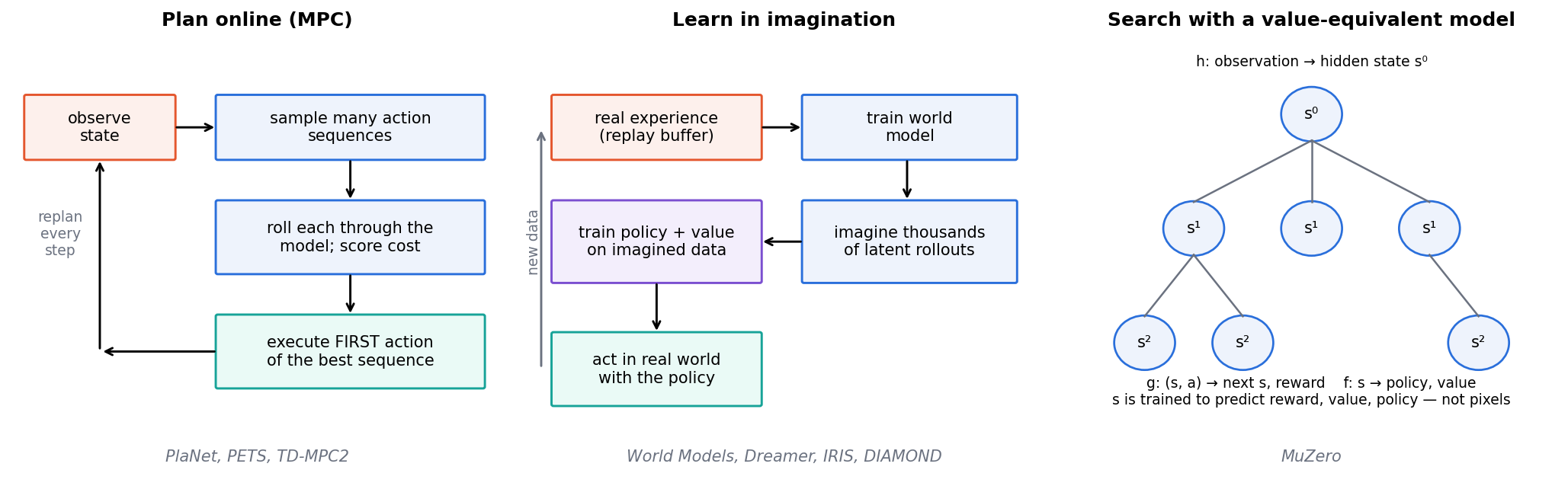
- Plan online (model-predictive control). At every real step, search for a good action sequence by simulating candidates in the model, execute only the first action, observe, and repeat. PlaNet [7], PETS [29] and TD-MPC2 [11] work this way.
- Learn in imagination. Train a policy (and usually a value function) on trajectories generated by the model, then act with that policy without searching at run time. World Models [6], the Dreamer line [8], [9], [10], IRIS [12] and DIAMOND [13] work this way.
- Search with a value-equivalent model. Learn a model that predicts only what planning needs (rewards, values, policy), not observations, and run tree search in its latent space. MuZero [14] is the canonical example.
All three share one danger: the model is wrong somewhere, and an optimizer is very good at finding exactly those places. We return to this in the section on uncertainty and exploitation.
Why errors compound
Each imagined step starts from the previous imagined step, so small prediction mistakes feed into the next prediction and can grow with every step.
Suppose the learned transition has one-step error at most , and the true dynamics are Lipschitz with constant (a small change in state changes the next state by at most times as much). Starting from the same state and applying the same actions, the gap between predicted and true states after steps obeys , so
For the bound grows exponentially with the horizon ; for it saturates at . This is a worst-case bound, but it explains two common design choices: replanning often (MPC) and using short model rollouts. Janner et al. made the second idea concrete: their MBPO algorithm branches short model rollouts from real states rather than imagining long trajectories from the start, and they argue both theoretically and empirically that this keeps the benefit of model data while limiting its bias [30].
World Models: compress, predict, control
Plain version. Encode observations, predict changes in that representation, and train a controller using the learned dynamics.
Ha and Schmidhuber’s World Models (published at NeurIPS 2018 as “Recurrent World Models Facilitate Policy Evolution”, with an interactive online version) made the idea popular in deep learning [6]. Their agent has three parts:
- V (vision): a variational autoencoder that compresses each frame into a small latent vector .
- M (memory): a recurrent network with a mixture-density output that predicts a distribution over given , the action and its hidden state .
- C (controller): a deliberately tiny linear policy , trained with an evolution strategy rather than backpropagation.
In a car-racing task, the controller using V and M features solved the task; in a VizDoom task, the controller was trained entirely inside the environment simulated by M and then transferred to the real game [6]. The design separates perception, prediction and decision, and shows that a controller can be very small when the representation already carries the relevant dynamics. It also showed the central risk: a controller trained inside an imperfect dream can learn to exploit the dream’s mistakes.
Latent dynamics: from PlaNet to the Dreamer line
Plain version. Instead of predicting future images, predict a compact hidden state and only decode images when training. A hidden state that mixes a deterministic memory with a random part can represent both what the agent remembers and what it is unsure about.
Recurrent state-space models
Hafner et al.’s PlaNet learned environment dynamics from images and chose actions by fast online planning in latent space; its key modeling idea is a latent dynamics model with both deterministic and stochastic components, the recurrent state-space model (RSSM) [7]. The RSSM keeps a deterministic memory and a stochastic state :
Here is a recurrent cell, the prior predicts without seeing the current image (this is what is used when imagining), and the posterior also sees the image (used during training and when filtering real observations). Heads read the model state to predict the image , the reward and a continuation flag (whether the episode goes on).
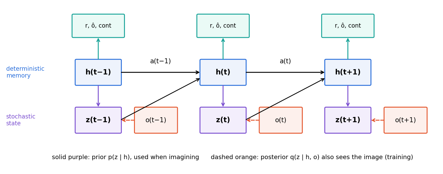
Training maximizes a variational lower bound on the likelihood of observed sequences. A simplified per-step loss is
with weighting the KL term. The reconstruction terms make the state informative; the KL term teaches the prior to predict what the posterior will see, which is exactly the skill needed for imagination. Real implementations add loss balancing and other stabilizers, so treat this as a teaching outline, not the exact loss of any one paper.
Optional: The ELBO and the reparameterization trick (in the Supplementary notes). Where this loss comes from and how gradients pass through the sampled state, with a one-variable example.
Dreamer: learning behavior in imagination
Dreamer (2020) kept the RSSM but replaced online planning with an actor–critic trained entirely on imagined latent trajectories. Its key move was to propagate analytic gradients of learned state values back through trajectories imagined in the compact latent space [8]. Starting from latent states inferred from real data, the agent imagines steps with its actor, scores them with a learned critic, and trains the critic on bootstrapped targets such as the -return
where and are the predicted reward and continuation, is the critic, and trades off one-step bootstrapping () against longer imagined returns (). The actor is updated to increase these values.
The line continued:
- DreamerV2 (2021) switched to discrete (categorical) latent variables and became the first agent to reach human-level performance on the 55-game Atari benchmark by learning behaviors inside a separately trained world model [9].
- DreamerV3 (Nature, 2025) used robustness techniques based on normalization, balancing and transformations so that a single configuration outperformed specialized methods across more than 150 tasks, and was the first algorithm to collect diamonds in Minecraft from scratch without human data or curricula [10].
Two related lines show that the RSSM is one choice among several. TD-MPC2 plans in the latent space of an implicit, decoder-free world model (no image reconstruction), reported strong results across 104 online RL tasks with a single set of hyperparameters, and trained a single 317M-parameter agent on 80 tasks [11]. IRIS replaced the RSSM with a discrete autoencoder plus an autoregressive Transformer over image tokens and learned from the equivalent of two hours of Atari gameplay [12]. DIAMOND went further toward pixels: it trains the agent inside a diffusion world model, arguing that discrete latents can drop visual details that matter for control, and also demonstrated the model as an interactive neural game engine for a 3D game [13].
MuZero: a model that predicts only what planning needs
Plain version. You do not have to predict what the screen will look like to play a good game. You only need to predict how good positions are, which moves look promising, and what rewards you will get. MuZero learns exactly that, and then searches.
AlphaZero-style tree search needs a simulator of the game rules. MuZero removes that requirement by learning a model that, applied repeatedly, predicts the quantities most directly relevant to planning: reward, action-selection policy and value [14]. It has three functions:
where (representation) encodes the observation history into a hidden state , (dynamics) maps a hidden state and a hypothetical action to a predicted reward and next hidden state, and (prediction) outputs a policy vector and a value . A Monte Carlo tree search unrolls to choose actions. Training unrolls the model for steps along real trajectories and minimizes
where are observed rewards, are value targets (bootstrapped returns), are the visit-count distributions produced by the search, are per-quantity losses and weights an L2 penalty.
The hidden state is never asked to reconstruct an observation. It only has to be value-equivalent: planning with it must give the same rewards, values and policies as planning in the real environment would. With this design MuZero reached a new state of the art on 57 Atari games and, without being given the rules, matched AlphaZero’s superhuman performance in Go, chess and shogi [14]. The lesson for vision is that a world model’s target should be chosen by its use; predicting every pixel is one option, not a requirement.
Video prediction and generation as world simulators
Plain version. If a model can generate realistic future video, perhaps it has learned how the world works. Sometimes it has; often it has only learned what videos usually look like. Testing which is the case is the hard part.
Action-conditioned video prediction
Finn et al. trained an action-conditioned video prediction model on a dataset of 59,000 robot pushing interactions; by predicting pixel motion rather than raw pixels, the model generalized partly to unseen objects, and conditioning on different future actions produced a “visual imagination” of different futures [15]. This is a world model in the most literal sense: image in, action in, image out.
Why squared-error predictors blur
Real futures are uncertain. Suppose that from the same past, a ball goes left with probability and right with probability . For squared error, the best single prediction is the conditional mean:
which here is two half-bright balls, an image that never happens. A generative model that samples one of the two futures produces a realistic image but, on average, a higher squared error.
Code · Python · 17 lines
import numpy as np

x = np.arange(64)
def frame(center):                      # a 1-D "image" with one bright ball
    return np.exp(-0.5 * ((x - center) / 2.0) ** 2)

# Same past, two equally likely futures: the ball bounces left or right.
futures = np.stack([frame(20), frame(44)])
mean_pred = futures.mean(axis=0)        # what an MSE-trained predictor converges to
sample_pred = futures[0]                # what a good generative sampler might output

def expected_mse(pred):                 # average over the two possible futures
    return np.mean([(pred - f) ** 2 for f in futures])

print(f"peak brightness: true future 1.00, mean prediction {mean_pred.max():.2f}")
print(f"expected MSE of mean prediction:   {expected_mse(mean_pred):.4f}")
print(f"expected MSE of a sharp sample:    {expected_mse(sample_pred):.4f}")
Output:
Code · 3 lines
peak brightness: true future 1.00, mean prediction 0.50
expected MSE of mean prediction:   0.0277
expected MSE of a sharp sample:    0.0554
The sharp sample has exactly twice the expected error of the blurry mean. This is why pixel MSE rewards blur, why stochastic video models were introduced, and why evaluating a world model with a single squared-error number can prefer the wrong model.
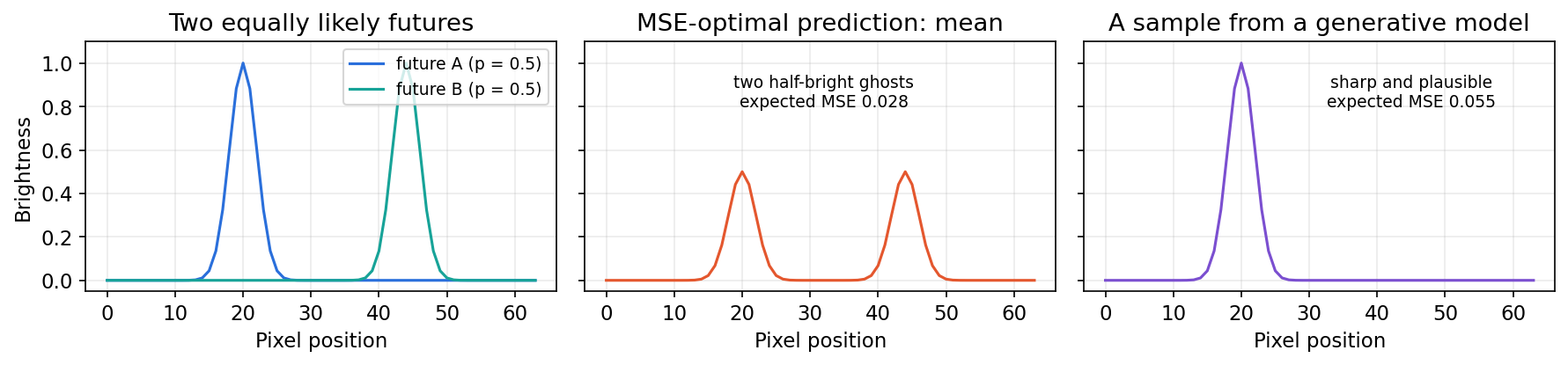
Babaeizadeh et al.’s SV2P addressed this by predicting a different possible future for each sample of a latent variable, and found substantially better predictions than the same model without stochasticity [16]. Modern video generators use the same principle at a much larger scale, with autoregressive token models or diffusion and flow models (see ML 08 and ML 09).
Large generative world models
Several large models now generate video conditioned on actions, text or actions inferred from the video itself, and are presented as world simulators.
- GAIA-1 casts driving world modeling as next-token prediction over discrete tokens of video, text and action, producing realistic driving scenarios with control over ego-vehicle behavior and scene features [17].
- UniSim learns a “universal simulator” of real-world interaction by combining datasets that are rich along different axes (objects in images, dense actions in robot data, motion in navigation data); it simulates both high-level instructions and low-level controls, and policies trained purely in it were deployed zero-shot on real robots [18].
- Genie is a generative interactive environment trained without action labels on unlabelled Internet video. It consists of a video tokenizer, an autoregressive dynamics model and a latent action model that infers actions from changes between frames, so users can act frame by frame in generated worlds even though no action labels were used in training [19]. Such latent actions need not correspond to calibrated physical actuators.
- Genie 3, announced by Google DeepMind in August 2025, generates worlds from text that can be navigated in real time at 24 frames per second and 720p, keeping consistency for a few minutes. The announcement lists limitations: a constrained action space, difficulty modeling several independent agents, inaccurate real-world locations, and interaction limited to minutes rather than hours [20].
- Cosmos is NVIDIA’s open platform of “world foundation models”: pretrained video models, video tokenizers, a data-curation pipeline and post-training examples meant to be fine-tuned into task-specific world models for robots and vehicles [21].
Does realistic video mean physical understanding?
Two careful studies say: not necessarily. Motamed et al.’s Physics-IQ benchmark tests fluid dynamics, optics, solid mechanics, magnetism and thermodynamics; across current video models (including Sora, Runway, Pika, Lumiere, Stable Video Diffusion and VideoPoet), physical understanding was severely limited and unrelated to visual realism [22]. Kang et al. trained diffusion video models on a 2D simulator governed by classical mechanics and found perfect in-distribution generalization, measurable scaling for combinatorial generalization, but failure out of distribution; the models behaved as if retrieving the closest training example rather than abstracting a rule [23].
For robot control, also ask what an “action” means: force, joint target, gripper command, camera movement or an inferred token. A wrong unit, timing offset or control frequency changes the conditional problem even if the video looks convincing.
Predictive representations: the JEPA family
Plain version. Predicting every pixel wastes effort on details that do not matter, like leaf texture. Instead, predict an abstract description of the missing or future part. If the description is good, the prediction is useful for planning.
A joint-embedding predictive architecture (JEPA) encodes a visible context and a hidden target with encoders, and trains a predictor to map the context embedding to the target embedding:
where is the context encoder, the target encoder, a predictor conditioned on information about where the target is (for example its position in the image or time), and (stop-gradient) blocks gradients into the target branch. Nothing is reconstructed in pixel space. The danger is collapse: if both encoders output a constant, the loss is zero. Asymmetric designs (a predictor on one side only, stop-gradient, and a target encoder that is not trained by the same gradient) are used to prevent it; ML 06 discusses these self-supervised mechanisms in more detail.
The JEPA line began as representation learning, on images (I-JEPA [24]) and then on video (V-JEPA [25]), and V-JEPA 2.1 [27] later refined its dense features. Two models show what turns it into a world model: action-conditioned prediction, and planning toward a goal in feature space.
- V-JEPA 2 pretrains an action-free JEPA on over one million hours of Internet video, then post-trains a latent action-conditioned world model, V-JEPA 2-AC, on less than 62 hours of unlabeled robot video; planning toward image goals with it enabled zero-shot pick-and-place on Franka arms in two labs without data from those environments, task-specific training or reward [26]. The split between passive video and action data makes the observation/action distinction of this chapter concrete.
- DINO-WM shows the same idea with an off-the-shelf encoder: it predicts future DINOv2 patch features from offline trajectories and plans by optimizing action sequences toward the features of a goal image, without reconstructing pixels or learning a reward model [28].
Optional: More of the JEPA line: I-JEPA, V-JEPA and V-JEPA 2.1 (in the Supplementary notes). What I-JEPA learned about masking, how V-JEPA trains on video alone, and what V-JEPA 2.1 adds for dense features.
Goals in feature space need care. A distance rewards only what the representation preserves. If the representation ignores gripper closure, a planner may reach a visually similar state without actually grasping the object. Better feature quality alone does not establish that an encoder predicts the consequences of arbitrary actions.
How the families relate
The families differ mainly in what they predict, and each prediction target raises its own question to test.
| Family | Prediction target | Main benefit | Question to test |
|---|---|---|---|
| Latent dynamics (RSSM, TD-MPC2) | compact state, reward, value | cheap, repeated rollouts | does the latent retain task-relevant dynamics? |
| Value-equivalent (MuZero) | reward, value, policy only | no effort on irrelevant detail | does it transfer when the reward changes? |
| Autoregressive video (GAIA-1, Genie, IRIS) | next frame or token | explicit sequential factorization | do errors drift over long rollouts? |
| Diffusion/flow video (DIAMOND, Cosmos) | jointly generated frames or chunks | expressive, uncertain futures | can actions steer outcomes at control latency? |
| Predictive embeddings (JEPA, DINO-WM) | target features | structure without pixel reconstruction | are actions represented and goals meaningful? |
These are compatible choices. A Transformer can parameterize any of them; a latent world model can decode through diffusion; a video generator can use an autoregressive outer loop and a diffusion inner loop. Architecture, prediction target, temporal factorization and training objective are separate design decisions.
Learning dynamics from data
Plain version. A dynamics model is only as good as its data: frames, actions and rewards must stay in order and correctly aligned, and test episodes must be truly separate from training ones.
Training examples should retain ordering and action alignment:
where marks the end of an episode. Record whether each action happens before or after each camera timestamp. Split by whole episodes, environment instances and relevant subjects; randomly splitting adjacent frames leaks nearly identical scenes and makes a transition predictor look better than it is (see ML 11 for leakage in general).
The data-collection policy matters. A model trained on slow, gentle interactions may fail for abrupt motion. Observational correlations are especially problematic when actions are absent: a model may learn that a cup moves when a hand approaches, yet have no evidence about what alternative pushes would do. This is the difference between passive video and interventional data.
A one-step loss measures prediction from real history. A multi-step loss unrolls the model’s own predictions and penalizes their accumulated error. Unrolling changes training difficulty and gradient paths; it does not remove distribution shift outside the observed interactions.
Complete CPU experiment: fit, predict, plan
Plain version. We now run the whole loop on a toy system: collect data, fit a model, check its predictions one step and many steps ahead, and plan with it.
We use a two-dimensional state , a scalar action and a damped linear system:
where is the state-transition matrix, the action-input vector and small Gaussian noise. The system is deliberately fully observed. It isolates dynamics and planning before adding image encoders and partial observability. Training and test episodes are generated independently. We fit only on training transitions and evaluate both one-step prediction and open-loop rollouts with the same held-out actions.
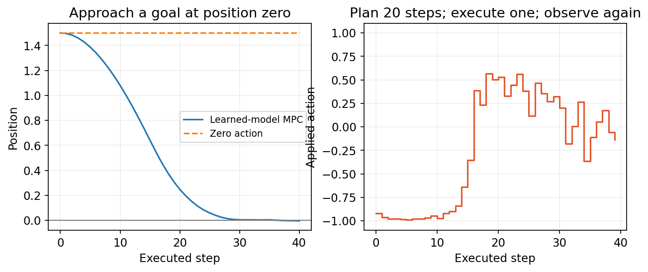
The planner uses the cross-entropy method (CEM): sample candidate action sequences from a Gaussian, keep the lowest-cost “elite” sequences under the model, refit the Gaussian’s mean and spread to them, and repeat. It executes one action, receives a fresh real state and replans. This is model-predictive control.
Optional: The cross-entropy method (in the Supplementary notes). The sample, rank and refit loop written out, with a small run on a known model.
Code · Python · 60 lines
import numpy as np

rng = np.random.default_rng(7)
A = np.array([[1.0, 0.1], [0.0, 0.94]])
B = np.array([0.005, 0.1])

def collect(n, steps=40):
    x = np.zeros((n, steps + 1, 2))
    x[:, 0] = rng.normal(size=(n, 2)) * [0.8, 0.3]
    u = rng.uniform(-1, 1, size=(n, steps))
    for t in range(steps):
        x[:, t + 1] = (x[:, t] @ A.T + u[:, t, None] * B
                       + rng.normal(scale=0.002, size=(n, 2)))
    return x, u

train, train_u = collect(120)
test, test_u = collect(80)
phi = np.column_stack([train[:, :-1].reshape(-1, 2), train_u.ravel()])
target = train[:, 1:].reshape(-1, 2)
W = np.linalg.lstsq(phi, target, rcond=None)[0]
W_no_action = np.linalg.lstsq(phi[:, :2], target, rcond=None)[0]

def predict(x, u):
    return np.concatenate([x, np.asarray(u)[..., None]], axis=-1) @ W

one_step = predict(test[:, :-1], test_u)
rollout = np.zeros_like(test)
rollout[:, 0] = test[:, 0]
for t in range(test_u.shape[1]):
    rollout[:, t + 1] = predict(rollout[:, t], test_u[:, t])
rmse = lambda a, b: np.sqrt(np.mean((a - b) ** 2))
print("One-step:", rmse(one_step, test[:, 1:]))
print("Without actions:", rmse(test[:, :-1] @ W_no_action, test[:, 1:]))
print("Final-horizon rollout:", rmse(rollout[:, -1], test[:, -1]))

def plan(x, mean, horizon=20, population=256):
    std = np.ones(horizon)
    for _ in range(4):
        candidates = np.clip(rng.normal(mean, std, (population, horizon)), -1, 1)
        imagined = np.broadcast_to(x, (population, 2)).copy()
        costs = np.zeros(population)
        for t in range(horizon):
            imagined = predict(imagined, candidates[:, t])
            costs += (imagined[:, 0] ** 2 + 0.15 * imagined[:, 1] ** 2
                      + 0.02 * candidates[:, t] ** 2)
        costs += 20 * imagined[:, 0] ** 2
        elite = candidates[np.argsort(costs)[:32]]
        mean = elite.mean(axis=0)
        std = elite.std(axis=0) + 0.05
    return mean

real = np.array([1.5, 0.0])
mean = np.zeros(20)
for _ in range(40):
    sequence = plan(real, mean)
    real = A @ real + B * sequence[0]  # real system; never used inside plan()
    mean = np.r_[sequence[1:], 0.0]
print("Controlled final state:", real)
assert rmse(one_step, test[:, 1:]) < 0.01
assert abs(real[0]) < 0.1
Output:
Code · 4 lines
One-step: 0.0019866110218121832
Without actions: 0.04106321931941812
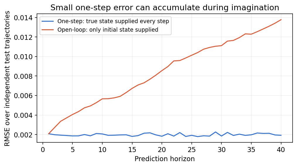
Final-horizon rollout: 0.013772759824274517
Controlled final state: [-0.00453985 -0.0210205 ]
The one-step RMSE () is at the noise level; dropping the action input raises it twentyfold (), so the action genuinely matters. The open-loop rollout error at horizon 40 () is about seven times the one-step error even for this nearly perfect linear model, a mild case of the compounding derived above. MPC drives the position from to about , compared with under zero action. These are synthetic results from this script, not published comparisons.
Replacing with an image embedding does not reproduce Dreamer or V-JEPA 2-AC: it adds an encoder-learning problem, latent uncertainty and the need for a valid goal or reward.
Planning, uncertainty and model exploitation
Plain version. A planner looks for the action the model likes best. If the model is wrong somewhere, the planner will happily go there. Knowing where the model is unsure is what keeps it honest.
A finite-horizon planning objective can be written as
where is a per-step cost, a terminal cost weighted by , and the expectation is over the model’s predicted latent states . Model-predictive control executes the first action, observes again and replans. Feedback corrects drift, but cannot rescue an action whose immediate consequence was badly modeled.
Two kinds of uncertainty
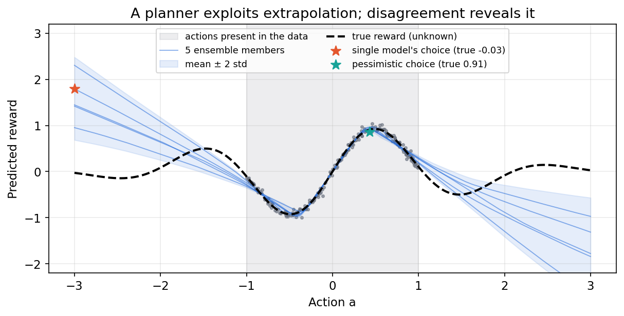
Aleatoric uncertainty is inherent randomness (a coin flip, the ball that may go left or right); more data does not remove it. Epistemic uncertainty comes from lack of data (the model has never seen this situation); more data does remove it. Sampling a generative model can represent aleatoric uncertainty, but sample diversity is not proof of calibration. Epistemic uncertainty is commonly approximated with ensembles: several models trained on bootstrap resamples or with different initializations agree where data is dense and tend to disagree where it is not. Chua et al.’s PETS combined probabilistic networks (for aleatoric noise) in an ensemble (for epistemic uncertainty) with sampling-based uncertainty propagation and CEM planning, matching the final performance of strong model-free methods on several benchmarks with far fewer samples [29].
Code: a planner exploiting a learned model
The agent has logged data only for actions in , but its planner may choose any action in .
Code · Python · 28 lines
import numpy as np
from sklearn.neural_network import MLPRegressor

rng = np.random.default_rng(0)
true_reward = lambda a: np.sin(3 * a) * np.exp(-0.3 * a ** 2)   # unknown to the agent

# Logged interactions only cover actions in [-1, 1].
a_data = rng.uniform(-1, 1, 200)
r_data = true_reward(a_data) + 0.05 * rng.normal(size=200)

ensemble = []
for k in range(5):                       # bootstrap + different initialization
    idx = rng.integers(0, 200, 200)
    m = MLPRegressor(hidden_layer_sizes=(64, 64), max_iter=3000, random_state=k)
    ensemble.append(m.fit(a_data[idx, None], r_data[idx]))

grid = np.linspace(-3, 3, 601)
preds = np.stack([m.predict(grid[:, None]) for m in ensemble])
mean, std = preds.mean(0), preds.std(0)

for name, score in [("single model", preds[0]),
                    ("ensemble mean", mean),
                    ("pessimistic: mean - 2 std", mean - 2 * std)]:
    a_star = grid[np.argmax(score)]       # the "planner": pick the best-looking action
    print(f"{name:26s} picks a = {a_star:+.2f}, predicted {score.max():.2f}, "
          f"true {true_reward(a_star):.2f}")
print(f"mean std inside data {std[np.abs(grid) <= 1].mean():.3f}, "
      f"outside {std[np.abs(grid) > 1.5].mean():.3f}")
Output:
Code · 4 lines
single model               picks a = -3.00, predicted 1.79, true -0.03
ensemble mean              picks a = -3.00, predicted 1.58, true -0.03
pessimistic: mean - 2 std  picks a = +0.43, predicted 0.87, true 0.91
mean std inside data 0.025, outside 0.321
Both the single model and the ensemble mean extrapolate a rising line outside the data, and the planner runs to the edge of the action space, where the true reward is about zero. Ensemble disagreement is thirteen times larger outside the data than inside, and a pessimistic score (mean minus two standard deviations) keeps the planner inside the data, where it finds an action with true reward . Restricting actions, shortening horizons, penalizing disagreement and testing with real feedback are the practical responses. Agreement among ensemble members is not proof of correctness, though: all five can share the same bias.
How to evaluate a world model
Plain version. No single number says whether a world model is good. Ask several questions, each with its own measurement and its own control.
| Question | Measurement | Important control |
|---|---|---|
| Does it predict known dynamics? | one-step and horizon-indexed state or feature error | independent episodes; fixed action sequence |
| Does appearance stay coherent? | reconstruction and video-quality metrics, identity consistency | compare camera motion and occlusions |
| Do actions matter correctly? | matched initial context with different specified actions | real action-conditioned reference trajectories |
| Are physical constraints respected? | collisions, object permanence, conservation; benchmarks such as Physics-IQ [22] | task-specific tolerances; out-of-distribution cases [23] |
| Does it help decisions? | success rate, return, interventions, control latency | test in the real or a trusted environment |
Pixel fidelity and decision usefulness can disagree, as the blur example showed. An averaged prediction can have low squared error while showing an impossible scene; an accurate latent predictor can omit visually irrelevant texture. Report the target, horizon, conditions and output resolution with every metric.
For comparison, include a persistence baseline (predict “nothing changes”), an action-free predictor and a simple task-appropriate dynamics model. Evaluate held-out objects, viewpoints, action ranges and environment properties separately. Report closed-loop control results in addition to imagined ones, and account for encoder and sampler latency: a planner that needs ten seconds per action may be useless for a robot running at 10 Hz.
Modern view
Plain version. Three lines of work now meet under the name “world model”: model-based reinforcement learning, video generators reframed as simulators, and predictive representations. The open questions are mostly about whether their predictions are reliable enough to act on.
Surveys. Moerland et al. give the most systematic treatment of model-based RL: dynamics-model learning (stochasticity, uncertainty, partial observability, temporal abstraction), a taxonomy of how planning and learning are integrated, and implicit (value-equivalent, MuZero-style) approaches [5]. Ding et al. (ACM Computing Surveys) organize the broader “world model” literature by function, understanding the world versus predicting its future, and review applications in generative games, autonomous driving, robotics and social simulation [1]. Zhu et al. survey “general world models” from the video-generation side, covering video generators, autonomous-driving world models and world models inside autonomous agents, and discuss their limitations [31]. Guan et al. give an initial survey of world models specifically for autonomous driving [32].
State of the art, 2023–2026.
- Model-based RL matured. DreamerV3 showed a single configuration working across more than 150 tasks and was published in Nature in 2025 [10]; TD-MPC2 showed decoder-free latent planning scaling to a multi-task 317M-parameter agent [11]; IRIS and DIAMOND showed Transformer and diffusion world models competitive on the Atari 100k benchmark [12], [13].
- Video generators were reframed as simulators. GAIA-1, UniSim, Genie, Genie 3 and Cosmos trained large models on video with actions, text or inferred latent actions [17], [18], [19], [20], [21]. The strongest evidence that they help agents is UniSim’s zero-shot transfer of policies trained inside the simulator [18]; the strongest caution is that realism does not imply physics [22], [23].
- Predictive representations moved toward control. The JEPA line went from images (I-JEPA) to video (V-JEPA) to action-conditioned planning on real robots (V-JEPA 2-AC) and denser features (V-JEPA 2.1) [24], [25], [26], [27]; DINO-WM showed that frozen self-supervised features can already support zero-shot planning [28].
Open problems.
- Long-horizon consistency. Errors compound; generated worlds drift; object identity and off-screen state are hard to keep for minutes, let alone hours [20].
- Causal and physical correctness. Models trained on passive video learn correlations; out-of-distribution physics fails [22], [23]. Interventional (action) data is scarce and expensive.
- Action interfaces. Latent actions inferred from video, robot joint commands and text instructions are different things; mapping between them reliably is unsolved.
- Exploitation and uncertainty. Planners and policies trained in imagination exploit model errors; calibrated epistemic uncertainty for large video models is largely missing.
- Evaluation. There is no agreed benchmark that ties prediction quality to downstream decision quality across domains; most papers still report either video metrics or task returns, rarely both.
- Cost. Sampling a large video model can be far slower than real time, which conflicts with closed-loop control.
Key takeaways
- The prediction target and action interface determine what a world model can support.
- Partial observations require memory or belief estimation; an image is not the full state.
- Planning, imagined policy training and value-equivalent search use learned dynamics differently.
- Pixel realism does not establish physical correctness; feature prediction also needs meaningful targets and anti-collapse mechanisms.
- Long rollouts compound errors, and optimization can exploit them; check uncertainty and replan.
- Evaluate held-out predictions, controlled action effects and behavior in the real environment.
Exercises
- Action ablation. In the CPU experiment, remove the action column. Compare one-step error, horizon-40 error and control behavior. Why can a short-term action-free predictor still look reasonable?
Hint
Imagined actions no longer affect the action-free predictor, so a planner cannot rank their consequences at all: every candidate gets the same predicted cost. Over one step the damped dynamics change the state only slightly, so persistence-like predictions still score moderately well, which is why one-step error alone is a weak test.
- Partial observations. Hide velocity and fit position-to-position dynamics. Then use the last two positions and the previous action as features. When does this history help, and where does observation noise hurt?
Hint
The difference of two positions estimates velocity (a finite difference), so the two-position model recovers most of the state. Noise in each position is amplified when divided by the time step, so the benefit shrinks as observation noise grows.
- Planning horizon. Compare horizons 5, 20 and 40, adjusting the initial mean to the chosen length. Measure final distance, action effort and runtime across several independent seeds.
Hint
Keep the cost definition fixed and count all model calls. Very short horizons cannot “see” that braking early avoids overshoot; very long horizons cost more and accumulate more model error, although for this linear system the error is small.
- Domain shift. Collect training episodes with velocity damping , then execute control in an environment with damping . Compare open-loop execution of a plan with replanning at every step. Identify an action range where the training data provide weak coverage.
Hint
Separate the learned dynamics (fitted on 0.94) from the true execution dynamics (0.75); do not refit on evaluation transitions. Replanning uses fresh observations, so it partially corrects the biased model; open-loop execution cannot.
- Mean versus sample. Extend the blur example to three equally likely futures at positions 10, 32 and 54. Compute the expected MSE of the mean prediction and of a single sharp sample. Then propose a metric that would prefer the sample.
Hint
The mean now has three one-third-height bumps; the expected MSEs are about (mean) and (sample), again a factor of two. That factor is general: if and are independent draws from the same distribution, , so a perfect sampler always has twice the MSE of the mean. A distribution-level metric (for example, comparing sets of generated samples with sets of real futures, as FID-style metrics do for images) or a best-of- error over several samples would reward sharp, plausible predictions.
- Pessimism trade-off. In the ensemble code, replace the factor 2 in “mean − 2 std” by 0, 0.5, 1 and 4. Plot the chosen action and its true reward for each. What goes wrong when the factor is too large?
Hint
At 0 the planner exploits extrapolation; as the factor grows it stays inside the data. Too much pessimism makes the planner avoid any action with even slight disagreement, so it may miss the best action inside the data and, in an RL setting, stop exploring.
References
- J. Ding et al., “Understanding world or predicting future? A comprehensive survey of world models,” ACM Computing Surveys, vol. 58, no. 3, 2025. doi arXiv
- C. M. Bishop, Pattern Recognition and Machine Learning, Springer, 2006, ch. 13 “Sequential Data”. book
- R. Szeliski, Computer Vision: Algorithms and Applications, 2nd ed., Springer, 2022. book
- R. S. Sutton, “Dyna, an integrated architecture for learning, planning, and reacting,” ACM SIGART Bulletin, vol. 2, no. 4, 1991. doi
- T. M. Moerland, J. Broekens, A. Plaat and C. M. Jonker, “Model-based reinforcement learning: a survey,” Foundations and Trends in Machine Learning, vol. 16, no. 1, 2023. doi arXiv
- D. Ha and J. Schmidhuber, “Recurrent world models facilitate policy evolution,” NeurIPS, 2018; interactive version “World Models,” arXiv:1803.10122. paper interactive
- D. Hafner et al., “Learning latent dynamics for planning from pixels,” ICML, 2019. paper
- D. Hafner, T. Lillicrap, J. Ba and M. Norouzi, “Dream to control: learning behaviors by latent imagination,” ICLR, 2020. arXiv
- D. Hafner, T. Lillicrap, M. Norouzi and J. Ba, “Mastering Atari with discrete world models,” ICLR, 2021. arXiv
- D. Hafner, J. Pasukonis, J. Ba and T. Lillicrap, “Mastering diverse control tasks through world models,” Nature, vol. 640, 2025. doi arXiv
- N. Hansen, H. Su and X. Wang, “TD-MPC2: scalable, robust world models for continuous control,” ICLR, 2024. arXiv
- V. Micheli, E. Alonso and F. Fleuret, “Transformers are sample-efficient world models,” ICLR, 2023. arXiv
- E. Alonso et al., “Diffusion for world modeling: visual details matter in Atari,” NeurIPS, 2024. arXiv
- J. Schrittwieser et al., “Mastering Atari, Go, chess and shogi by planning with a learned model,” Nature, vol. 588, 2020. doi arXiv
- C. Finn, I. Goodfellow and S. Levine, “Unsupervised learning for physical interaction through video prediction,” NIPS, 2016. arXiv
- M. Babaeizadeh, C. Finn, D. Erhan, R. H. Campbell and S. Levine, “Stochastic variational video prediction,” arXiv:1710.11252, 2017. arXiv
- A. Hu et al., “GAIA-1: a generative world model for autonomous driving,” technical report, arXiv:2309.17080, 2023. arXiv
- S. Yang et al., “Learning interactive real-world simulators,” arXiv:2310.06114, 2023. arXiv
- J. Bruce et al., “Genie: generative interactive environments,” arXiv:2402.15391, 2024. arXiv
- Google DeepMind, “Genie 3: a new frontier for world models,” blog post, August 5, 2025. blog
- NVIDIA (N. Agarwal et al.), “Cosmos world foundation model platform for physical AI,” arXiv:2501.03575, 2025. arXiv
- S. Motamed, L. Culp, K. Swersky, P. Jaini and R. Geirhos, “Do generative video models understand physical principles?,” arXiv:2501.09038, 2025. arXiv
- B. Kang et al., “How far is video generation from world model: a physical law perspective,” ICML, 2025. arXiv
- M. Assran et al., “Self-supervised learning from images with a joint-embedding predictive architecture,” CVPR, 2023. doi arXiv
- A. Bardes et al., “Revisiting feature prediction for learning visual representations from video,” arXiv:2404.08471, 2024. arXiv
- M. Assran et al., “V-JEPA 2: self-supervised video models enable understanding, prediction and planning,” arXiv:2506.09985, 2025. arXiv
- L. Mur-Labadia et al., “V-JEPA 2.1: unlocking dense features in video self-supervised learning,” arXiv:2603.14482, 2026. arXiv
- G. Zhou, H. Pan, Y. LeCun and L. Pinto, “DINO-WM: world models on pre-trained visual features enable zero-shot planning,” arXiv:2411.04983, 2024. arXiv
- K. Chua, R. Calandra, R. McAllister and S. Levine, “Deep reinforcement learning in a handful of trials using probabilistic dynamics models,” NeurIPS, 2018. arXiv
- M. Janner, J. Fu, M. Zhang and S. Levine, “When to trust your model: model-based policy optimization,” NeurIPS, 2019. arXiv
- Z. Zhu et al., “Is Sora a world simulator? A comprehensive survey on general world models and beyond,” arXiv:2405.03520, 2024. arXiv
- Y. Guan et al., “World models for autonomous driving: an initial survey,” arXiv:2403.02622, 2024. arXiv
- D. P. Kingma and M. Welling, “Auto-encoding variational Bayes,” International Conference on Learning Representations (ICLR), 2014; arXiv:1312.6114. arXiv
- D. J. Rezende, S. Mohamed and D. Wierstra, “Stochastic backpropagation and approximate inference in deep generative models,” ICML, 2014. paper
- R. Y. Rubinstein, “The cross-entropy method for combinatorial and continuous optimization,” Methodology and Computing in Applied Probability, vol. 1, no. 2, 1999. doi
- P.-T. de Boer, D. P. Kroese, S. Mannor and R. Y. Rubinstein, “A tutorial on the cross-entropy method,” Annals of Operations Research, vol. 134, no. 1, 2005. doi
Check your understanding
This tutorial has 6 exercises. Can you solve them without opening the hints?
Go to the exercises ↑Next DLCV 14 · Robustness: Distribution Shift, Adversarial Examples and Anomalies · 42 min