DLCV 12A · Video Generation
Needs: DLCV 12 · Image Generation: From GANs to Text-to-Image Systems
Navigate: this page and this track: Navigate: this page and this track
On this page
- What you’ll learn1 min
- The big picture2 min
- What makes video harder than images2 min
- Compressing video: 3D VAEs and video tokenizers5 min
- Architectures: from inflated image models to video transformers7 min
- Conditioning: text-to-video and image-to-video2 min
- Camera and motion control1 min
- Long videos2 min
- Temporal consistency4 min
- Autoregressive and diffusion video generation3 min
- Evaluating video generators4 min
- Data1 min
- Risks and responsible use1 min
- Failure modes1 min
- Modern view2 min
- Key takeaways1 min
- Exercises3 min
- Supplementary notes
- Paper guides
- References
Deep Learning for Computer Vision
What you’ll learn
- Separate frame quality, motion quality and temporal consistency.
- Understand spatial/temporal compression and token-budget tradeoffs.
- Compare temporal extensions of image models with video-native attention.
- Trace text, image, camera and motion conditions through long-video generation.
- Evaluate joint-clip and streaming models with complementary metrics and human studies.
The big picture
A video generator makes a short moving picture from a request: a sentence (“a dog runs along a beach at sunset”), a still image to bring to life, a camera path, or the first seconds of a clip to continue. The result must look good in every frame, the motion must be believable, and things must stay the same thing from one frame to the next.
Why it matters. Video generation is used in creative tools, for animating photos, for generating training data and simulation scenes, and as a candidate “world simulator” for robots and vehicles. It is also the most expensive kind of visual generation: a five-second clip contains dozens of images that must all agree. Most of the engineering is about one trade-off: modeling all frames jointly, for consistency, without paying for every pixel of every frame to interact with every other.
Where this chapter sits. The image side is covered elsewhere and is not repeated. DLCV 12 explains text encoders, cross-attention, guidance in practice, control and editing, text-to-image evaluation and risks. ML 08 derives diffusion, classifier-free guidance, latent diffusion, diffusion transformers, flow matching and few-step samplers, and its section Video adds temporal compression and a consistency problem is the short preview that this chapter expands. ML 09 covers autoregressive generation and visual tokenizers. DLCV 13 discusses action-conditioned video prediction, large generative world models and whether realistic video implies physical understanding. DLCV 09A.3 introduces optical flow, warping and temporal-consistency measures. Here we focus on what is specific to generating video. All code runs in seconds on a CPU with NumPy, SciPy and scikit-image, without network weights.
What makes video harder than images
Plain version. Video generation must produce good frames, plausible motion and consistent identities. Independent high-quality frames can still form a flickering video.
The tasks
Every task below samples a video (with frames of height and width , three color channels) from a conditional distribution ; the tasks differ only in the condition .
| Task | Condition | Examples in this chapter |
|---|---|---|
| Text-to-video (T2V) | a text prompt | Make-A-Video [1], CogVideoX [2], Wan [3] |
| Image-to-video (I2V) | a first frame, often plus a prompt | Stable Video Diffusion [4], DynamiCrafter [5] |
| Video extension or prediction | earlier frames of the same clip | VDM [6], Video LDM [7], StreamingT2V [8] |
| Frame interpolation | keyframes to fill in between | Make-A-Video [1], Stable Video Diffusion [4] |
| Video editing | an input video plus an edit request | Tune-A-Video [9], Text2Video-Zero [10] |
| Controlled generation | a camera path or object trajectories | MotionCtrl [11], CameraCtrl [12], DragNUWA [13] |
As with images (DLCV 12), one trained model can often serve several rows: a first frame, earlier frames or keyframes are extra conditions, and masking decides which frames are generated.
Three demands on every clip
- Per-frame quality. Each frame on its own should look like a real image: sharp, free of artifacts, well composed.
- Motion quality. The clip should move, and the motion should be plausible: speed, direction and deformation should look like the real thing. A clip that barely moves is a failure even if every frame is perfect.
- Temporal consistency. What is the same object should stay the same object. Three failures have names. Flicker is fast, frame-to-frame change of brightness or fine texture that no real motion explains. Identity drift is a slow change of a subject’s appearance (a face, a logo, the pattern on a shirt) over the clip. A failure of object permanence is an object that disappears, changes or reappears wrongly after being hidden.
The demands pull against each other. The easiest way to remove flicker is to generate almost no motion; the easiest way to get dramatic motion is to let details change freely. Evaluation, later in this chapter, has to check all three together.
The cost
A video is large. A clip of frames at pixels (about five seconds at 16 frames per second) holds numbers, the size of about 81 images. A generator also cannot simply treat the frames one after another: consistency requires information to flow between distant frames. With attention, the cost of letting every position see every other position grows with the square of the number of positions. Two design levers control it: compress the video before generating (the next section), and restrict which positions attend to which (the section after it).
Compressing video: 3D VAEs and video tokenizers
Plain version. Video autoencoders compress space and time to reduce generation cost. Their reconstruction quality limits recoverable detail and motion.
Why not compress each frame with an image autoencoder?
The first latent video models reused the autoencoder of an image latent diffusion model [14] and encoded every frame separately. The Video LDM authors report that this causes flickering, because the image autoencoder was trained on images only and does not know that consecutive frames should decode consistently; they fine-tuned the decoder with added temporal layers and a 3D-convolutional discriminator on video, and found this step critical for good results [7]. Stable Video Diffusion also builds on a pretrained image latent model and compresses only in space [4], [3]. A frame-wise autoencoder also keeps one latent frame per video frame, so it does nothing for the cost in time.
3D causal VAEs
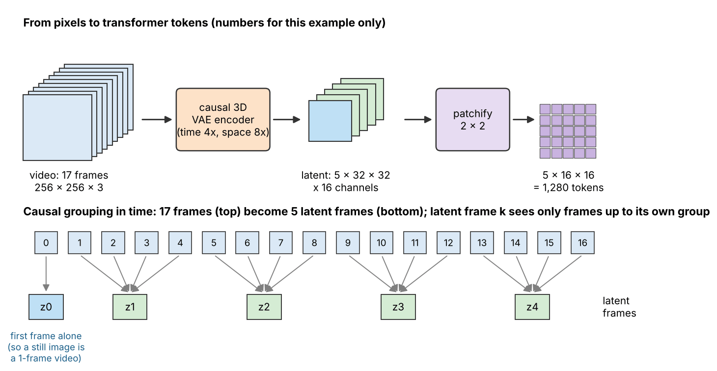
A 3D VAE uses convolutions over time as well as space, so it can downsample both [2]. Most recent systems make it causal in time: every temporal convolution is padded only at the beginning of the clip, so a latent frame depends only on the current and earlier video frames, never on later ones [15], [2]. A useful consequence is that the very first frame is encoded on its own. The usual frame layout is therefore "": the first frame becomes the first latent frame, and every following group of frames becomes one more latent frame. A still image is then just a one-frame video, which lets one autoencoder, and one generator, train on images and videos together [15], [16], [3].
Let a clip have frames of size , compressed by a factor in time and along each spatial axis into latent channels. The latent grid and the number of transformer tokens are
where , and are the numbers of latent frames, rows and columns, is the side of the square patch that the transformer groups into one token (often ), and is the sequence length. Wan’s report gives exactly this count, , for its autoencoder and patches [3]. Two numbers summarize a design: the compression of numbers, , and the pixels per token, about . Because the latent has more channels than the 3 of RGB, a video VAE compresses tokens much more than it compresses numbers.
Figure 1 shows the arithmetic for a 17-frame clip.
Published systems document their factors. The table lists a few (a map of choices, not a ranking).
| System | Compression (time × height × width) | Latent channels | Notes |
|---|---|---|---|
| Stable Video Diffusion [4] | 1 × 8 × 8 | 4 | image autoencoder, no temporal compression (factors as listed in [3]) |
| CogVideoX [2] | 4 × 8 × 8 | 16 | 3D causal VAE |
| HunyuanVideo [16] | 4 × 8 × 8 | 16 | causal 3D VAE, -frame input |
| Wan [3] | 4 × 8 × 8 | 16 | causal; first frame compressed only in space |
| Movie Gen [17] | 8 × 8 × 8 | 16 | temporal autoencoder inflated from an image autoencoder |
| LTX-Video [18] | 8 × 32 × 32 | 128 | about 1:192 overall; no separate patchify step |
| MAGVIT-v2 in VideoPoet [19] | 17 frames of 128 × 128 → 5 × 16 × 16 discrete tokens | vocabulary of | discrete tokens for a language model |
LTX-Video frames the comparison in pixels per token: a autoencoder followed by patches gives 1,024 pixels per token, while its own design gives 8,192 [18]. Pushing compression further has a price. CogVideoX’s ablation found that a setting made the generator’s training converge with great difficulty even with more latent channels [2], and LTX-Video asks its decoder to perform the final denoising step in pixel space to recover fine detail lost by the strong compression [18].
Optional: Causal 3D convolutions and the 1 + T frame layout (in the Supplementary notes). How causal padding works, why the first frame is independent, and how strided convolutions map frames to .
Continuous latents or discrete tokens
Like image models (DLCV 12), video generators either work on a continuous latent grid (a VAE, used by diffusion and flow models) or on discrete tokens from a learned codebook (used by masked and autoregressive token models). MAGVIT introduced a 3D tokenizer that quantizes a video into spatiotemporal tokens for masked generation [20]. MAGVIT-v2 replaced it with a causal 3D CNN tokenizer and a lookup-free quantizer whose vocabulary can grow large, and with it a language model outperformed diffusion models on image and video benchmarks in the authors’ tests [15]; codebooks and their problems are covered in ML 09.
Code: latent size and attention cost
The snippet computes the latent grid, the number of tokens and the number of query–key pairs in one attention layer for an 81-frame, clip, for three autoencoders. The pair counts anticipate the next section: “full” lets every token attend to every token, “factorized” splits attention into a spatial part within each latent frame and a temporal part at each position.
Code · Python · 22 lines
def latent_grid(frames, height, width, ft, fs, channels=16):
    """Latent shape of a causal video VAE: the first frame alone, then groups of ft frames."""
    t = 1 + (frames - 1) // ft
    return t, height // fs, width // fs, channels

def attention_pairs(t, s):
    """Query-key pairs in one attention layer over t latent frames of s tokens each."""
    full = (t * s) ** 2                 # every token attends to every token
    factorized = t * s**2 + s * t**2    # spatial attention per frame + temporal attention per position
    return full, factorized

frames, H, W, patch = 81, 480, 832, 2   # about 5 s at 16 fps; DiT patches of 2 x 2 latent positions
pixels = frames * H * W * 3
print(f"pixel values: {pixels:,}")
for name, ft, fs, c in [("image VAE, every frame", 1, 8, 4),
                        ("video VAE 4x8x8", 4, 8, 16),
                        ("video VAE 8x16x16", 8, 16, 64)]:
    t, h, w, c = latent_grid(frames, H, W, ft, fs, c)
    s = (h // patch) * (w // patch)     # tokens per latent frame after patchify
    full, fact = attention_pairs(t, s)
    print(f"{name:23s} latent {t}x{h}x{w}x{c} ({pixels / (t*h*w*c):5.1f}x fewer numbers)  "
          f"tokens {t*s:7,}  full {full:.1e}  factorized {fact:.1e}  ratio {full/fact:4.0f}")
It prints:
Code · 4 lines
pixel values: 97,044,480
image VAE, every frame  latent 81x60x104x4 ( 48.0x fewer numbers)  tokens 126,360  full 1.6e+10  factorized 2.1e+08  ratio   77
video VAE 4x8x8         latent 21x60x104x16 ( 46.3x fewer numbers)  tokens  32,760  full 1.1e+09  factorized 5.2e+07  ratio   21
video VAE 8x16x16       latent 11x30x52x64 ( 88.4x fewer numbers)  tokens   4,290  full 1.8e+07  factorized 1.7e+06  ratio   11
(All numbers are our own arithmetic; the row with 64 channels is a hypothetical configuration, not a specific model.) Three lessons. First, the video VAE keeps about as many numbers as the frame-wise image VAE, but it cuts the tokens by a factor of four, and the attention pairs by a factor of sixteen, because each latent position carries more channels. Second, the 32,760 tokens match Wan’s formula for this clip size. Third, full attention over 32,760 tokens means about query–key pairs per layer, which is why the choice between full and factorized attention, and the compression factor, decide what a model can afford.
Architectures: from inflated image models to video transformers
Plain version. One route adds temporal layers to an image model; another trains a video Transformer. Both must decide how information crosses space and time.
Inflating a pretrained image model
The idea is to reuse what an image model already knows about appearance and to learn only motion. Video Diffusion Models (VDM) turned the image diffusion U-Net into a 3D U-Net factorized over space and time: every convolution became a convolution that acts on each frame separately, each spatial attention block kept attending within a frame, and a new temporal attention block after it attended over frames at each spatial position [6]. Because temporal attention can be switched off, the same network can be trained on single images and on videos at once, and the authors found this joint training important for sample quality [6].
Later systems keep the pretrained image layers and insert new temporal layers that are initialized to do nothing, so the inflated model starts exactly as the image model. Let be the features of one block, reshaped so that frames are treated as a batch of images. The inflated block computes
where attends along the frame axis at each spatial position and is a linear projection whose weights start at zero, so that at the start of training (the same idea as ControlNet’s zero convolutions in DLCV 12). Training then moves the model gradually from “a batch of independent images” toward “a video”. Make-A-Video [1], Video LDM [7], AnimateDiff [21] and Open-Sora [22] all use a version of this idea: identity-initialized layers, a learned mixing weight or zero-initialized projections. Make-A-Video also shows the payoff: it learns appearance and its link to text from image–text pairs and only motion from unlabeled video, so it needs no paired text–video data [1].
Optional: Four ways to start a video model from an image model (in the Supplementary notes). What Make-A-Video, Video LDM, AnimateDiff and Open-Sora each freeze, add and initialize.
Factorized or full spatiotemporal attention
Plain version. A token can look at every other token in the clip (full attention), or first at the tokens of its own frame and then at the tokens in the same place in other frames (factorized attention). Factorized attention is much cheaper; full attention can follow an object that moves far between frames.
Let a clip have latent frames of tokens each, so tokens in total. One full attention layer compares query–key pairs. Factorized attention runs spatial attention inside each frame ( problems of size , so pairs) and temporal attention at each position ( problems of size , so pairs). The ratio is
which is close to when , as in the snippet above (ratio 21 for 21 latent frames). The factorized pattern comes from video understanding: TimeSformer compared self-attention schemes and found “divided” space–time attention best among those it tried for video classification [23], and ViViT proposed several variants that factorize the spatial and temporal dimensions [24]. Latte compared four such decompositions inside a latent video diffusion transformer (interleaved spatial and temporal blocks, late fusion, and two ways of splitting attention inside a block) and found interleaved spatial and temporal transformer blocks performed best in its experiments [25].
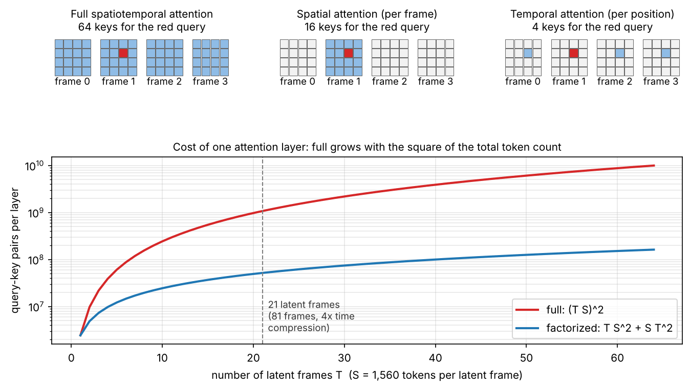
The case for full attention is about motion. CogVideoX argues that with separated spatial and temporal attention, an object that moves far between adjacent frames cannot attend directly to itself in the next frame; information must travel indirectly through other patches, which makes consistency of large motions hard to learn; it therefore uses full 3D attention over text and video tokens together [2]. HunyuanVideo chose full attention, citing better results than divided attention, a single design for images and videos, and the reuse of acceleration methods developed for language models [16]. Wan also uses full spatiotemporal attention [3]; Open-Sora Plan moved from a factorized “2+1D” denoiser to 3D full attention and added a cheaper sparse attention operation [26]; and LTX-Video uses its very high compression precisely so that full attention stays affordable [18]. The practical rule: full attention is preferred when the token count allows it, and the autoencoder is designed to make the token count allow it.
Cascades or one model for the whole clip
Cascades generate a short, small, low-frame-rate video and then improve it with separate models. Imagen Video uses seven sub-models (one base model, three spatial super-resolution and three temporal super-resolution models) to reach 128 frames of at 24 frames per second, about 5.3 seconds [27]. Make-A-Video combines a base model, a frame-interpolation network and two super-resolution models [1]; Video LDM generates sparse keyframes and fills in frames with an interpolation model [7]. A cascade keeps each stage small, but the base stage fixes the global motion from few frames. Lumiere argued that generating distant keyframes and then interpolating makes global temporal consistency difficult, and introduced a Space-Time U-Net that downsamples and upsamples in time as well as space and generates the full-frame-rate clip in one pass [28]. Large latent transformers with temporal compression take the same single-stage route; Movie Gen notes that its temporal compression lets it forgo the frame-interpolation models of earlier work [17].
A map of landmark systems
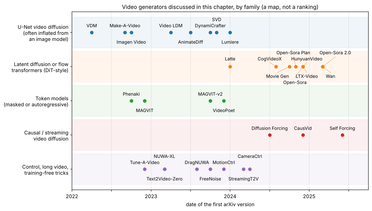
The table lists systems whose design is documented in a paper or technical report. It is a map of design choices, not a ranking; Figure 3 places them in time.
| System | Generator and backbone | Where it generates | Note |
|---|---|---|---|
| VDM [6] | diffusion, factorized 3D U-Net | pixels | joint image–video training |
| Make-A-Video [1] | diffusion, inflated U-Net, cascade | pixels | no paired text–video data |
| Imagen Video [27] | diffusion, cascade of seven models | pixels | spatial and temporal super-resolution |
| Video LDM [7] | diffusion, frozen image LDM plus temporal layers | image-autoencoder latent | fine-tuned temporal decoder |
| Stable Video Diffusion [4] | diffusion, inflated latent U-Net | image-autoencoder latent | staged training with data curation |
| Lumiere [28] | diffusion, Space-Time U-Net | pixels | whole clip in one pass |
| Latte [25] | diffusion transformer, factorized | latent | compares four factorizations |
| CogVideoX [2] | diffusion transformer, full 3D attention | 3D causal VAE latent | text and video tokens concatenated |
| Open-Sora [22] | diffusion transformer, factorized (STDiT) | 3D autoencoder latent | fully open training code and weights |
| Open-Sora Plan [26] | diffusion transformer, 3D attention with a cheaper sparse variant (Skiparse) | wavelet-flow VAE latent | open project with data pipeline |
| HunyuanVideo [16] | flow-matching transformer, full attention | causal 3D VAE latent | over 13 billion parameters |
| Movie Gen [17] | flow-matching transformer | temporal-autoencoder latent | 30B parameters, synchronized audio |
| Wan [3] | flow-matching diffusion transformer, full attention | causal 3D VAE latent | 1.3B and 14B models |
| LTX-Video [18] | latent diffusion transformer, full attention | highly compressed latent | decoder does the last denoising step |
| MAGVIT [20], VideoPoet [19] | masked or autoregressive token transformer | discrete tokens | see the section on autoregressive generation |
Flow matching and diffusion transformers are derived in ML 08 and ML 08, diffusion transformers [29], [30]. Parameter counts above are the ones stated in the papers.
Conditioning: text-to-video and image-to-video
Plain version. The prompt enters a video model the same way it enters an image model, through attention to text-encoder outputs. A first frame for image-to-video enters as an extra input that every generated frame can see. The difference from images is that the condition must hold for the whole clip, and that “how much it moves” is itself something to control.
Text-to-video
Text encoders, cross-attention and joint text–image attention are explained in DLCV 12. Video systems use the same mechanisms. Wan embeds text with cross-attention from video tokens to text-encoder outputs [3]. CogVideoX concatenates text and video tokens in one sequence and uses an expert adaptive LayerNorm with separate modulation for the two modalities, because their feature spaces and numerical scales differ [2]. HunyuanVideo processes video and text tokens in separate streams first and then concatenates them for joint processing (“dual-stream to single-stream”), with a multimodal language model as its main text encoder [16]. Captions must describe motion and events, not only appearance (see Data).
Make-A-Video also feeds the frame rate to the model, as data augmentation and as a control of motion speed [1]. Guidance works as for images (DLCV 12).
Image-to-video
Image-to-video (“animate this photo”) must keep the input frame’s content while inventing motion. Three documented designs:
- Stable Video Diffusion replaces the text embedding with the image embedding of the conditioning frame from a pretrained image–text model, and concatenates a noise-augmented copy of the frame to the denoiser input along the channel axis, repeated for every frame. The authors found that a constant guidance scale caused either drift away from the conditioning frame or oversaturation, and instead increased the guidance scale linearly across frames [4].
- DynamiCrafter projects the image into a text-aligned context space with a query transformer, so that the video model can attend to it like a prompt, and also concatenates the full image with the initial noise to preserve visual detail [5].
- HunyuanVideo uses the latent of the reference image directly as the first latent frame [16], a natural choice when the causal VAE encodes the first frame alone.
A common failure of image-to-video is too little motion: the model can score well on fidelity to the input by barely changing it. StreamingT2V reports that competing image-to-video models tend toward “video stagnation” when used repeatedly to extend a clip [8].
Camera and motion control
Plain version. A prompt such as “the camera slowly orbits the statue” is a weak way to describe motion. Control methods give the generator the motion directly: a camera path (where the camera is in each frame) or trajectories (where an object or a dragged point should go). The challenge is to obey the motion without changing the content.
- Camera motion as a small adapter. Stable Video Diffusion trained separate camera-motion LoRA modules for horizontal movement, zooming and a static camera on top of its base model [4]; AnimateDiff’s MotionLoRA adapts its motion module to new motion patterns such as shot types at a low cost [21].
- Camera poses as a dense input. CameraCtrl trains a plug-and-play camera module on top of a video diffusion model, leaving the base model untouched. Instead of feeding raw camera matrices, it represents each frame’s camera as a per-pixel Plücker embedding, a 6-number description of the viewing ray through each pixel, which ties camera geometry to image positions; the authors found that training videos with diverse camera paths and an appearance similar to the base model’s data gave the best balance of control and generalization [12].
- Camera and objects together. MotionCtrl controls camera motion and object motion independently, with camera poses and object trajectories as conditions that carry no appearance information [11]. DragNUWA combines text, an image and trajectories for fine-grained control of open-domain video [13].
A camera path is the same pose sequence that 3D reconstruction estimates (DLCV 11). Following it does not make the generated scene geometrically consistent, and a control signal is only as reliable as the poses or tracks it was trained on.
Optional: Camera poses as Plücker embeddings (in the Supplementary notes). What the six numbers per pixel mean, and how translation and rotation change them, with a tested snippet.
Long videos
Plain version. Models are trained on short clips, a few seconds long, because memory grows with length. To make a longer video you must either keep extending a clip piece by piece, which tends to drift, or plan the whole video coarsely first and fill in the details, which needs long training videos. Either way, keeping the story and the identities straight over a minute is still hard.
Four strategies are documented:
- Extend autoregressively, chunk by chunk. Generate a clip, then generate the next clip conditioned on the last frames of the previous one. VDM showed that simply replacing the known frames during sampling gives continuations that look good alone but do not match the earlier frames, and proposed reconstruction guidance, which adds a guidance term from the model’s reconstruction of the conditioning frames [6]. Video LDM trains prediction models that receive a few context frames through a mask [7]. StreamingT2V adds a short-term memory (attention to features of the previous chunk) for smooth transitions and a long-term memory (features of the first chunk) so the model does not forget the initial scene [8].
- Plan coarse, then fill in. NUWA-XL applies a global diffusion model to generate keyframes over the entire time range and local diffusion models that recursively fill in frames between them, which lets it train directly on long videos and generate segments in parallel [31].
- Change the noise, not the model. FreeNoise extends a pretrained short-clip model without tuning: it reschedules a sequence of initial noises with long-range correlation and applies temporal attention over windows, and adds a motion-injection method for prompts that change over time [32].
- Variable-length generation from a story. Phenaki compresses video into discrete tokens with a tokenizer that is causal in time, so it handles variable lengths, and generates long videos from a sequence of prompts that change over time [33].
The central difficulty is error accumulation: each chunk is conditioned on generated, slightly wrong frames, and errors compound, exactly as in the rollouts of a learned world model (DLCV 13). The causal-diffusion methods in the section on autoregressive generation address the same problem from the training side.
Optional: Reconstruction guidance for extending a video (in the Supplementary notes). Why replacing the known frames is not enough, and the correction term VDM adds.
Temporal consistency
Plain version. A consistent video keeps each detail attached to the thing it belongs to: when the dog moves, its spots move with it; when the camera pans, the texture of the wall slides along. The simplest test is to undo the motion and check that nothing else changed. The trap is that a video that does not move at all passes this test perfectly.
Where inconsistency comes from
A generator invents detail that the condition does not specify. If that invented detail is drawn afresh for every frame, it flickers. If it is fixed to the screen instead of to the objects, it “sticks” while the scene moves under it. Consistency means the invented detail must be propagated along the motion. Architectures do this through temporal layers and joint generation of all frames; several training-free methods enforce it in pretrained image models. Text2Video-Zero makes the self-attention of every frame attend to the first frame (cross-frame attention), to preserve the appearance and identity of the foreground object, and adds motion dynamics to the latent codes to keep the background consistent [10]. Make-A-Video uses the same noise initialization for every frame in its final per-frame super-resolution stage, to encourage consistent invented detail across frames [1]. Tune-A-Video adds a spatiotemporal attention mechanism to an image model and tunes it on a single video [9].
Measuring consistency
Three measures are common, and each is defined in terms of quantities you can compute from the generated video alone:
- Frame difference , where is frame and the number of pixel values per frame. It is cheap but mixes real motion with flicker; VBench measures temporal flickering this way only on static scenes, where all change is flicker [34].
- Warping error , where is the motion (optical flow) from frame to frame and warps the previous frame along it. It removes the real motion before comparing; flow, warping and its masked form are explained in DLCV 09A.3. For a generated video the flow must be estimated from the video itself.
- Feature similarity over time. VBench’s subject consistency compares the features of each frame with those of the first and the previous frame, , where is a unit-length feature vector of frame from a self-supervised image model and is the dot product (cosine similarity) [34].
All three reward a still video. For that reason VBench pairs them with a dynamic degree dimension that measures the amount of motion with an optical-flow network [34].
Code: flicker, sticking and freezing
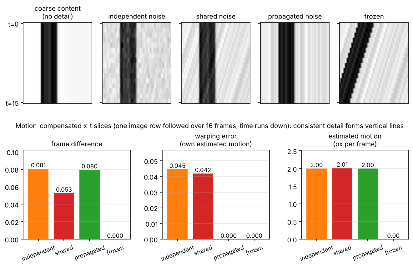
The toy builds a “coarse video” that pans an image 2 pixels per frame, as a prompt might request, and adds invented fine detail in four ways: new noise every frame, the same noise fixed on the screen, the same noise moved along with the scene, and a frozen video that repeats the first frame. It estimates each video’s own motion with phase correlation and reports the three quantities.
Code · Python · 33 lines
import numpy as np
from scipy import ndimage as ndi
from skimage import data, transform
from skimage.registration import phase_cross_correlation

rng = np.random.default_rng(0)
T, v = 16, 2                                   # 16 frames; the prompt asks for a pan of 2 px per frame
scene = transform.resize(data.camera() / 255.0, (128, 128), anti_aliasing=True)
content = np.stack([np.roll(scene, v * t, axis=1) for t in range(T)])   # the "coarse" video

def detail():                                  # invented fine texture, as a generator would add
    n = ndi.gaussian_filter(rng.standard_normal(scene.shape), 0.7)
    return 0.04 * n / n.std()

d0 = detail()
videos = {
    "independent noise": content + np.stack([detail() for _ in range(T)]),  # new detail every frame
    "shared noise":      content + d0,                                       # same detail, fixed on screen
    "propagated noise":  content + np.stack([np.roll(d0, v * t, axis=1) for t in range(T)]),  # detail moves with the scene
}
videos["frozen"] = np.repeat(videos["propagated noise"][:1], T, axis=0)      # a still image repeated

c = (slice(None), slice(8, -8), slice(8, -8))  # ignore borders (np.roll wraps around)
def measure(vid):
    shifts = [phase_cross_correlation(a, b, upsample_factor=10)[0][1] for a, b in zip(vid[1:], vid[:-1])]
    flicker = np.abs(np.diff(vid, axis=0))[c].mean()                         # frame-difference energy
    warped = np.stack([np.roll(f, int(round(s)), axis=1) for f, s in zip(vid[:-1], shifts)])
    warp_err = np.abs(vid[1:] - warped)[c].mean()                            # error after the video's own motion
    return flicker, warp_err, np.mean(np.abs(shifts))

for name, vid in videos.items():
    f, w, m = measure(vid)
    print(f"{name:18s} frame difference {f:.4f}   warping error {w:.4f}   estimated motion {m:.2f} px/frame")
It prints:
Code · 4 lines
independent noise  frame difference 0.0808   warping error 0.0446   estimated motion 2.00 px/frame
shared noise       frame difference 0.0528   warping error 0.0419   estimated motion 2.01 px/frame
propagated noise   frame difference 0.0796   warping error 0.0000   estimated motion 2.00 px/frame
frozen             frame difference 0.0000   warping error 0.0000   estimated motion 0.00 px/frame
(All numbers are from our toy run.) Read the four lines together:
- Frame difference alone is misleading. It rates the screen-fixed noise (0.0528) as more stable than the correct, propagated detail (0.0796), because the propagated detail moves, and it gives the frozen video a perfect zero.
- Warping error separates the cases that move. After undoing the estimated motion, only the propagated detail leaves nothing behind; both new-every-frame noise and screen-fixed noise remain visible.
- A motion measure is needed as well. The frozen video also has zero warping error. Only the estimated motion (0.00 instead of the requested 2 pixels per frame) exposes it, which is the role of VBench’s dynamic degree.
Figure 4 shows the same effects as motion-compensated x–t slices: correct, propagated detail forms straight vertical lines.
Autoregressive and diffusion video generation
Plain version. There are two ways to produce a clip. A diffusion (or flow) model refines all frames of a fixed-length clip together, from noise to video, so every frame can see the future as well as the past. An autoregressive model writes the video piece by piece, each piece conditioned on what came before, like a language model writing text; it can go on as long as you like and can stream, but early mistakes stay. Recent hybrids try to get both.
Token models: masked and autoregressive
With a discrete video tokenizer, video generation becomes sequence modeling (ML 09). MAGVIT uses masked token modeling, predicting many tokens in parallel, and supports many generation tasks (such as frame prediction, interpolation and inpainting) with a single model [20]. Phenaki generates its causal video tokens with a bidirectional masked transformer conditioned on text [33]. VideoPoet is a decoder-only transformer that processes text, image, video and audio tokens; MAGVIT-v2 turns 17 frames of video at 8 frames per second into a grid, that is 1,280 tokens from a vocabulary of , and the model is trained like a language model, with pretraining on a mixture of generative tasks followed by task-specific adaptation [19]. Token models reuse language-model infrastructure (KV caching, ML 09) and can extend a clip naturally, but every generated token is a commitment, and errors accumulate (ML 09).
Diffusion: the whole clip at once
A standard video diffusion transformer denoises all latent frames jointly with bidirectional attention. CausVid states the consequence plainly: generating a single frame requires processing the entire sequence, including the future, which makes such models hard to use interactively [35]. Their strengths are the ones that made diffusion dominant for images (stable training, high quality, guidance), plus global consistency within the clip. Their limits are a fixed maximum length and high latency.
Hybrids: causal, streamable diffusion
- Diffusion Forcing trains a diffusion model to denoise a sequence of tokens with independent noise levels per token, and uses it as a causal next-token model that generates future frames without fully diffusing past ones; this allows rolling out video beyond the training horizon, where its baselines diverge [36].
- CausVid adapts a pretrained bidirectional video diffusion transformer into a causal, autoregressive one that generates frames on the fly, distills its 50-step sampler into a 4-step one with a bidirectional teacher supervising the causal student, and uses KV caching for streaming generation; the authors report that this mitigates error accumulation and allows long videos despite training on short clips [35].
- Self Forcing attacks exposure bias directly: during training, each frame is generated conditioned on the model’s own previous outputs (an autoregressive rollout with KV caching), not on ground-truth frames, and a loss is applied to the whole generated video; it reports real-time streaming generation with sub-second latency on a single GPU [37].
| Aspect | Autoregressive or causal | Bidirectional diffusion |
|---|---|---|
| Length | open-ended, chunk by chunk | fixed by the training clip length, unless extended |
| Latency | first frames available early, can stream | whole clip must be denoised first |
| Future information | none (causal) | every frame sees past and future |
| Main risk | error accumulation, exposure bias | memory and compute for long clips |
| Typical use | interactive generation, world models, live video | offline text-to-video and image-to-video |
The same causal-versus-bidirectional distinction matters for world models, where actions arrive one step at a time (DLCV 13). Remember also, from ML 08, that a causal autoencoder does not make a generator autoregressive: the generator’s attention and sampling decide that.
Evaluating video generators
Plain version. You need evidence of four things: that the videos as a set look like real videos (distribution metrics such as FVD), that they match their prompts, that their motion and consistency are good (dimension-by-dimension suites such as VBench), and that people prefer them (human studies). The standard distribution metric turns out to look mostly at single frames, so it can miss exactly the temporal problems this chapter is about.
Fréchet Video Distance
FVD extends FID (ML 08) to video [38]. Each video, real or generated, is passed through a pretrained video network, an I3D action-recognition model [39] trained on Kinetics-400 [40], and its output (the logits) is taken as a feature vector. A Gaussian is fitted to each set of features, and
where are the mean and covariance of the real-video features, those of the generated videos, is the trace and the matrix square root. Lower is better. The original paper introduced FVD with a human study in which it correlated well with judgments of generated videos [38]. Class-conditional and unconditional benchmarks often report FVD on UCF-101, a dataset of 101 human-action classes [41], [1], [25].
Its main limit: content bias. Ge et al. found that FVD increases only slightly under large temporal corruption at matched frame quality, and that a well-chosen subset of generated videos without motion can lower FVD drastically [42]. They trace the bias to the features: an action classifier trained on Kinetics learns object and scene appearance, because many actions can be recognized from one frame; features from a self-supervised video model, VideoMAE v2 [43], were much less biased [42]. The pitfalls of FID also apply (DLCV 12), plus video-specific ones: clip length, frame rate and resizing to a low, square resolution [42].
Optional: Ge et al., “On the Content Bias in Fréchet Video Distance” (in the Paper guides). How the paper separates frame quality from motion quality, and how to read its sensitivity plots.
Code: a Fréchet distance that cannot see time
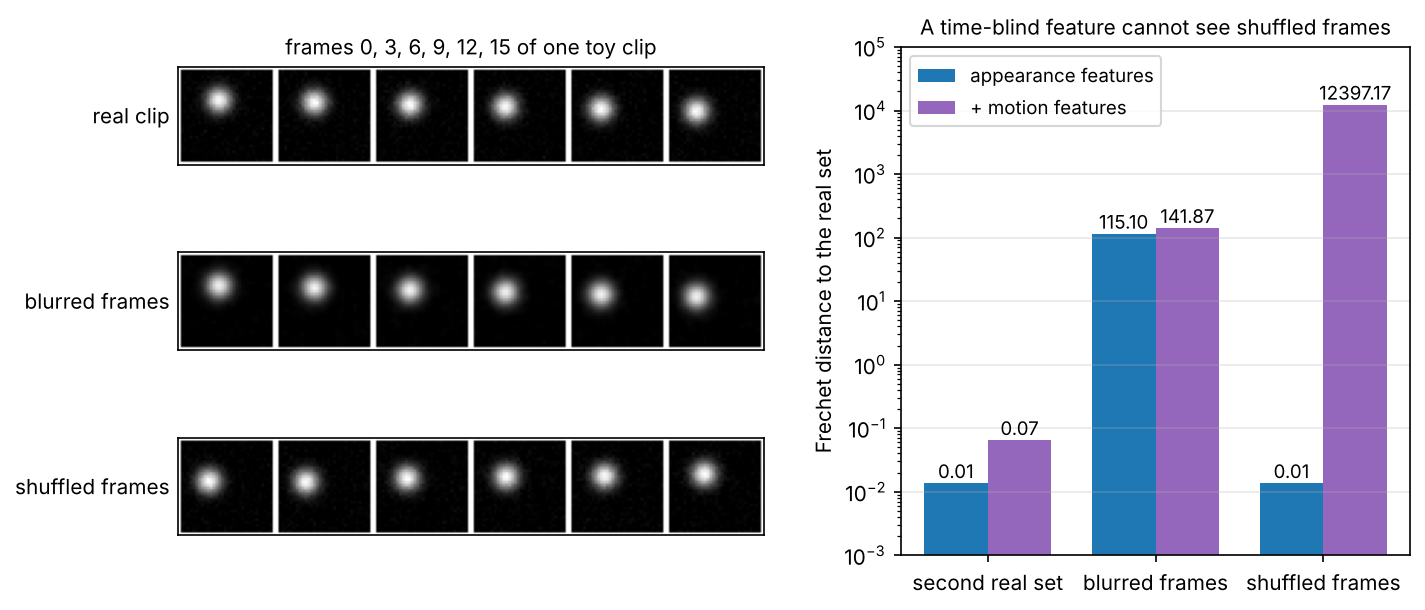
The toy makes “real” clips of a blob moving in a straight line and two corrupted sets: one with blurred frames (worse frames, correct motion) and one with shuffled frames (perfect frames, broken motion). It computes a Fréchet distance with two hand-made feature extractors: one that averages per-frame appearance statistics over time, like an extractor that mostly sees content, and one that adds two temporal statistics.
Code · Python · 45 lines
import numpy as np
from scipy import linalg, ndimage as ndi

rng = np.random.default_rng(0)
T, S = 16, 32
yy, xx = np.mgrid[:S, :S]

def real_videos(n):
    """Toy 'real' clips: a bright blob moving in a straight line, plus mild sensor noise."""
    vids = np.empty((n, T, S, S))
    for i in range(n):
        p, vel, r = rng.uniform(10, 22, 2), rng.uniform(-0.7, 0.7, 2), rng.uniform(2.5, 4)
        for t in range(T):
            cy, cx = p + vel * t
            vids[i, t] = np.exp(-((yy - cy) ** 2 + (xx - cx) ** 2) / (2 * r**2))
    return vids + 0.02 * rng.standard_normal(vids.shape)

def frame_stats(f):                      # appearance of one frame
    gy, gx = np.gradient(f)
    return [f.mean(), f.std(), f.max(), np.abs(gx).mean() + np.abs(gy).mean()]

def appearance_features(v):              # frame statistics averaged over time: blind to frame order
    return np.mean([frame_stats(f) for f in v], axis=0)

def motion_features(v):                  # add how the content changes from frame to frame
    d = np.abs(np.diff(v, axis=0)).mean(axis=(1, 2))
    return np.concatenate([appearance_features(v), [d.mean(), d.std()]])

def frechet(a, b):                       # Fréchet distance between Gaussian fits of two feature sets
    mu1, mu2 = a.mean(0), b.mean(0)
    s1, s2 = np.cov(a, rowvar=False), np.cov(b, rowvar=False)
    covmean = linalg.sqrtm(s1 @ s2).real
    return float(((mu1 - mu2) ** 2).sum() + np.trace(s1 + s2 - 2 * covmean))

real, other_real = real_videos(400), real_videos(400)
blurred = ndi.gaussian_filter(other_real, sigma=(0, 0, 0.7, 0.7))          # worse frames, same motion
shuffled = np.stack([v[rng.permutation(T)] for v in other_real])          # perfect frames, broken motion

for name, feats in [("appearance features", appearance_features), ("+ motion features", motion_features)]:
    f = lambda vids: np.stack([feats(v) for v in vids])
    ref = f(real)
    scale = ref.std(0)                   # put all features on a comparable scale
    fd = {k: frechet(ref / scale, f(v) / scale) for k, v in
          [("second real set", other_real), ("blurred frames", blurred), ("shuffled frames", shuffled)]}
    print(f"{name:20s} " + "   ".join(f"{k} {d:6.2f}" for k, d in fd.items()))
It prints:
Code · 2 lines
appearance features  second real set   0.01   blurred frames 115.10   shuffled frames   0.01
+ motion features    second real set   0.07   blurred frames 141.87   shuffled frames 12397.17
(All numbers are from our toy run, with toy features, not I3D.) With appearance-only features, the shuffled set, whose motion is destroyed, is exactly as close to the real set as a second real set (0.01), while mild blur is heavily penalized. Adding two temporal statistics makes the shuffled set by far the worst. The real FVD is not this extreme, since I3D does see some motion, but this is the shape of the content bias that Ge et al. measured [42]: the metric is only as temporal as its features. Figure 5 shows the clips and the distances.
Benchmark suites and human evaluation
Plain version. Instead of one number, modern benchmarks ask many narrow questions, each with its own prompts and its own automatic check, and confirm that the checks agree with people.
- VBench splits “video generation quality” into 16 dimensions, each with tailored prompts and an evaluation method: temporal quality (subject consistency, background consistency, temporal flickering, motion smoothness, dynamic degree), frame-wise quality (aesthetic and imaging quality), semantics (object class, multiple objects, human action, color, spatial relationship, scene), style (appearance and temporal style) and overall consistency; it provides human preference annotations for each dimension to validate the automatic scores [34]. VBench++ extends it to image-to-video, with an image suite of adaptive aspect ratio, and to trustworthiness [44].
- EvalCrafter builds 700 prompts from an analysis of real user data, evaluates visual quality, content quality, motion quality and text–video alignment with 17 objective metrics, and fits coefficients so that the combined score agrees with users’ opinions [45].
- Human evaluation remains the reference. Stable Video Diffusion compares its training choices with human preference studies [4]; HunyuanVideo reports evaluations by professionals [16]; Movie Gen evaluates with pairwise A/B tests by expert annotators along text alignment, visual quality, and realness and aesthetics, over a public set of 1,003 prompts, and reports that FVD and Inception Score did not correlate with its human evaluation of video quality [17]. Open-Sora 2.0 reports both human evaluation and VBench scores [46].
Physical plausibility needs its own tests; DLCV 13 describes benchmarks that found physical understanding unrelated to visual realism.
A reporting checklist. State the prompts and how they were chosen, the clip length, frame rate and resolution, the number of samples and seeds, the sampler, steps and guidance (including any schedule across frames), the feature extractor and preprocessing of every distribution metric, the dimension suite and its version, and the human-study protocol (pairwise or absolute, number of annotators, majority rule). Report a temporal measure together with a motion measure and a per-frame quality measure, and show uncurated clips.
Data
Plain version. Video models learn appearance, motion and the link to language from their training clips. Video with good captions is much scarcer than captioned images, so systems combine image and video data and spend great effort on filtering and recaptioning clips.
- Images plus videos. VDM [6], Phenaki [33] and many later systems train jointly on images and videos; Make-A-Video learns text–visual links only from image–text pairs [1]; the causal "" autoencoders make images one-frame videos [16], [3].
- Web video collections. WebVid, web videos with weak captions, was introduced with the Frozen in Time retrieval model (WebVid-2M in the paper; a 10M version was released later, according to its arXiv record) [47], and Make-A-Video was trained on WebVid-10M [1]. Panda-70M curates 3.8M high-resolution videos, splits them into semantically consistent clips and captions them with several cross-modality teacher models plus a retrieval model that selects the best caption, giving 70M clips with captions [48].
- Curation matters. Stable Video Diffusion’s Large Video Dataset starts with 580M annotated clips, forming 212 years of content, then removes nearly static clips with optical-flow scores, clips with much written text by OCR, and clips with low aesthetic scores; models trained on curated subsets were preferred by people over models trained on uncurated data [4]. CogVideoX describes its own video-captioning model as a key part of its data pipeline [2].
- Evaluation datasets. UCF-101 [41] and Kinetics [40] are human-action datasets that supply FVD benchmarks and FVD’s feature network.
Optional: Stable Video Diffusion (in the Paper guides). How one paper turns data curation and staged training into controlled experiments, and how to read its human-preference plots.
Web video raises the same questions of copyright, consent and content safety as web images; see DLCV 12, Data.
Risks and responsible use
Plain version. Realistic generated video can put words in someone’s mouth or show events that never happened. The defenses are the same three as for images (detect fakes, label generated content, and limit misuse at the source), but video is harder: it is re-encoded on every upload, and a few convincing seconds are enough to mislead.
- Deepfakes and detection. FaceForensics++ is a benchmark for detecting facial manipulations (four manipulation methods at random compression levels and sizes, over 1.8 million manipulated images, with a hidden test set); its authors found that domain-specific knowledge improves detection even under strong compression and that the detectors outperform human observers on their benchmark [49]. Detectors trained on one generation method can fail on newer ones, so detection is an arms race.
- Watermarks for video. Video Seal jointly trains a watermark embedder and extractor with transformations such as video codecs applied in between, and propagates the watermark over time so that not every high-resolution frame has to be watermarked [50]. Signed provenance manifests, invisible watermarks and their failure modes are explained in DLCV 12, Deepfakes, provenance and watermarks and its note Hard bindings, soft bindings and watermarks; the same lessons apply to video, where re-encoding and cropping are routine.
- Bias, memorization and consent follow from the data as for images (DLCV 12, Risks); people appear in web video far more often than in many image collections, which raises the stakes of consent.
- False authority. A generated video that looks physically right is easily taken as evidence. Treat generated clips as illustrations, not records, and see DLCV 13 on why realism is not physical correctness.
Failure modes
Plain version. Today’s video generators are good at short, single-shot clips of common scenes. They still fail at keeping things the same over time, at physics, at fine-grained motion and at anything long.
- Flicker and texture sticking. Fine detail changes from frame to frame or stays fixed while the scene moves (Figure 4).
- Identity drift and morphing. Faces, text and patterns change slowly; two objects merge or one object splits.
- Object permanence. Objects vanish when occluded or come back different.
- Too little motion. Near-static clips that score well on consistency; dynamic-degree measures exist because of this [34], and image-to-video extension can stagnate [8].
- Implausible physics and dynamics. Motion looks fluid but is physically wrong (see DLCV 13).
- Drift in long videos. Error accumulation when extending clip by clip [35], [37]; forgetting of the initial scene [8].
- Weak control. Camera paths that are only roughly followed, trajectories that change object shape; MotionCtrl’s design goal of appearance-free motion conditions targets exactly this [11].
- Inherited image failures. Counting, attribute binding, text rendering and hands fail as in images (DLCV 12, Failure modes), now with the extra chance of changing over time.
How to test. Build small prompt sets per failure type (fast motion, occlusion, a person turning around, written text, a requested camera move), generate several seeds per prompt, measure consistency and motion, inspect motion-compensated x–t slices for flicker and sticking, and watch the clips; a frame grid hides most temporal failures.
Modern view
Surveys worth reading.
- Melnik et al. [51] (TMLR 2024) survey video diffusion models: the mathematical formulation, architectural choices, methods for temporal consistency, a taxonomy of applications by input modality (text, images, video, audio), training and evaluation practice with datasets and metrics, and open challenges such as long videos and computational cost.
- Xing et al. [52] (2023) review video diffusion models in three areas, video generation, video editing and other video understanding tasks, with further categories in each, and discuss challenges and future trends.
- Liu et al. [53] (2024) review OpenAI’s Sora, introduced in February 2024, from public technical reports and reverse engineering: background, related technologies, applications and limitations such as safe and unbiased generation. Because it relies on reverse engineering, read its technical claims as informed hypotheses.
Historical models versus available services. The papers here explain architectural milestones, not a current purchasing shortlist. As checked on 5 November 2026, OpenAI states that Sora’s web/app experiences ended on 26 April 2026 and its API ended on 24 September 2026 [54]. The independent Open-Sora projects are different projects. For current deployment choices and the checks that matter to a shot, see the video-generation selection guide.
State of the art, 2023–2026. Five trends stand out. (1) Latent transformers with full attention and causal 3D VAEs became the dominant recipe for large open models (CogVideoX [2], HunyuanVideo [16], Wan [3]), with flow-matching objectives in several of them [16], [17], [3]. (2) Open models report closing much of the gap with closed systems in their own human evaluations and VBench scores, and training cost became a research topic: Open-Sora 2.0 reports training a commercial-level model for about $200k [46]. (3) Higher compression reduces tokens so that full attention stays affordable, with the decoder taking over more of the detail [18]. (4) Causal, few-step, streaming generation brought interactive and real-time use [35], [37], [36]. (5) Evaluation moved beyond FVD toward dimension suites [34], [44], [45] and large human studies [17], with a recognized need for temporally sensitive features [42]. Synchronized audio generation also appeared [17], [19].
Open problems. Consistency and identity over minutes rather than seconds; physically correct dynamics and interaction (DLCV 13); precise, disentangled control of camera, objects and timing; metrics that measure motion and consistency without rewarding stillness and that agree with people; the cost of training and sampling long, high-resolution clips; caption quality for events and actions; and provenance that survives re-encoding.
Key takeaways
- A sharp frame is not enough: motion and identity must remain coherent across time.
- Compression reduces generation cost but limits recoverable detail and temporal information.
- Temporal layers, factorized attention and full space–time attention offer different communication patterns and costs.
- State what is conditioned: text, the first frame, camera pose or motion trajectory.
- Chunk extension and causal generation enable longer outputs but must manage accumulated errors.
- Evaluate appearance, motion, temporal consistency and preference together; report data curation, duration and full cost.
Exercises
- Token budgets. A model uses a causal VAE and patches. How many tokens does a 121-frame clip at produce? How many query–key pairs does one full attention layer have, and by what factor does factorized attention reduce it? Which single change, doubling the temporal compression or doubling the patch size, reduces the full-attention cost more?
Hint
, and each latent frame has tokens, so tokens and about pairs. The factorized ratio is . Doubling gives (pairs shrink about 3.8×); doubling divides the tokens per frame by 4 (pairs shrink 16×), at the cost of coarser spatial tokens. Use the snippet’s functions to check.
- Break the consistency measures. In the consistency toy, add a fifth video in which the propagated detail is shifted by 2 pixels per frame but the coarse content does not move (a “moving texture on a still scene”). What do the three measures report, and which of them would you trust to detect this failure?
Hint
Phase correlation now sees two competing motions: the texture moves, the content does not. Depending on their relative strength, the estimated shift is 0 or 2, and whichever layer is not compensated leaves a warping error. A single global motion estimate is not enough for real videos with several moving parts; dense optical flow with occlusion masks is used in practice (DLCV 09A.3).
- Content bias in your own features. Modify the Fréchet toy so that the “generated” set has correct frames but the blob moves twice as fast as in the real set. Which feature extractor detects it? Then design a third feature that would also detect a blob that moves at the right speed but reverses direction halfway.
Hint
Speed changes the mean frame difference, so only the motion features detect it. A reversal keeps the mean absolute difference similar; a feature that compares the direction of motion over time (for example the correlation between the first and second halves of the centroid trajectory, or the net displacement divided by the path length) is needed. Real metrics face the same question: which temporal properties do the features encode?
- Choose an architecture. You must build an image-to-video model for product photos (a slow 3-second camera orbit around an object) with a small video dataset and a strong pretrained image model. Choose between inflating the image model with factorized temporal layers and training a full-attention video transformer from scratch, and say how you would add camera control.
Hint
With little video and a strong image model, inflation with zero- or identity-initialized temporal layers reuses appearance knowledge and needs less data; camera motion is slow, so factorized attention’s weakness with large motion matters less. Condition on the photo (concatenated latent plus an image embedding, as in Stable Video Diffusion) and add a camera module with per-pixel Plücker embeddings, trained on clips with diverse, known camera paths. Evaluate identity preservation of the product across frames, camera-path accuracy and a dynamic-degree measure.
- Evaluation plan. A team claims its new model has “better temporal consistency” because its VBench subject-consistency score is higher. List three alternative explanations and the additional evidence you would ask for.
Hint
The model might move less (check dynamic degree and motion smoothness), might generate simpler or shorter clips (check prompts, clip length and frame rate), or might differ in frame quality that affects the feature extractor (check frame-wise quality). Ask for the full dimension table with the same VBench version, uncurated clips per prompt, a human pairwise study on consistency with motion held comparable, and FVD with a temporally sensitive feature extractor.
References
- U. Singer, A. Polyak, T. Hayes et al., “Make-A-Video: Text-to-Video Generation without Text-Video Data,” arXiv:2209.14792, 2022. arXiv
- Z. Yang, J. Teng, W. Zheng et al., “CogVideoX: Text-to-Video Diffusion Models with An Expert Transformer,” ICLR, 2025. arXiv
- Team Wan, A. Wang, B. Ai, B. Wen et al., “Wan: Open and Advanced Large-Scale Video Generative Models,” arXiv:2503.20314, 2025. arXiv
- A. Blattmann, T. Dockhorn, S. Kulal et al., “Stable Video Diffusion: Scaling Latent Video Diffusion Models to Large Datasets,” arXiv:2311.15127, 2023. arXiv
- J. Xing, M. Xia, Y. Zhang et al., “DynamiCrafter: Animating Open-Domain Images with Video Diffusion Priors,” ECCV, LNCS, pp. 399–417, 2024. doi · arXiv
- J. Ho, T. Salimans, A. Gritsenko, W. Chan, M. Norouzi and D. J. Fleet, “Video Diffusion Models,” NeurIPS, 2022. proceedings · arXiv
- A. Blattmann, R. Rombach, H. Ling et al., “Align your Latents: High-Resolution Video Synthesis with Latent Diffusion Models,” CVPR, 2023. CVF
- R. Henschel, L. Khachatryan, H. Poghosyan et al., “StreamingT2V: Consistent, Dynamic, and Extendable Long Video Generation from Text,” CVPR, 2025. CVF
- J. Z. Wu, Y. Ge, X. Wang et al., “Tune-A-Video: One-Shot Tuning of Image Diffusion Models for Text-to-Video Generation,” ICCV, 2023. CVF
- L. Khachatryan, A. Movsisyan, V. Tadevosyan et al., “Text2Video-Zero: Text-to-Image Diffusion Models are Zero-Shot Video Generators,” ICCV, 2023. CVF
- Z. Wang, Z. Yuan, X. Wang et al., “MotionCtrl: A Unified and Flexible Motion Controller for Video Generation,” SIGGRAPH 2024 Conference Papers, 2024. doi · arXiv
- H. He, Y. Xu, Y. Guo et al., “CameraCtrl: Enabling Camera Control for Text-to-Video Generation,” ICLR, 2025. arXiv
- S. Yin, C. Wu, J. Liang et al., “DragNUWA: Fine-grained Control in Video Generation by Integrating Text, Image, and Trajectory,” arXiv:2308.08089, 2023. arXiv
- R. Rombach, A. Blattmann, D. Lorenz, P. Esser and B. Ommer, “High-Resolution Image Synthesis with Latent Diffusion Models,” CVPR, 2022. CVF
- L. Yu, J. Lezama, N. B. Gundavarapu et al., “Language Model Beats Diffusion — Tokenizer is Key to Visual Generation,” ICLR, 2024. arXiv
- W. Kong, Q. Tian, Z. Zhang et al., “HunyuanVideo: A Systematic Framework For Large Video Generative Models,” arXiv:2412.03603, 2024. arXiv
- A. Polyak, A. Zohar, A. Brown et al., “Movie Gen: A Cast of Media Foundation Models,” arXiv:2410.13720, 2024. arXiv
- Y. HaCohen, N. Chiprut, B. Brazowski et al., “LTX-Video: Realtime Video Latent Diffusion,” arXiv:2501.00103, 2024. arXiv
- D. Kondratyuk, L. Yu, X. Gu et al., “VideoPoet: A Large Language Model for Zero-Shot Video Generation,” ICML, PMLR 235, 2024. PMLR · arXiv
- L. Yu, Y. Cheng, K. Sohn et al., “MAGVIT: Masked Generative Video Transformer,” CVPR, 2023. CVF
- Y. Guo, C. Yang, A. Rao et al., “AnimateDiff: Animate Your Personalized Text-to-Image Diffusion Models without Specific Tuning,” ICLR, 2024. arXiv
- Z. Zheng, X. Peng, T. Yang et al., “Open-Sora: Democratizing Efficient Video Production for All,” arXiv:2412.20404, 2024. arXiv
- G. Bertasius, H. Wang and L. Torresani, “Is Space-Time Attention All You Need for Video Understanding?,” ICML, PMLR 139, 2021. PMLR
- A. Arnab, M. Dehghani, G. Heigold, C. Sun, M. Lučić and C. Schmid, “ViViT: A Video Vision Transformer,” ICCV, 2021. CVF
- X. Ma, Y. Wang, X. Chen et al., “Latte: Latent Diffusion Transformer for Video Generation,” Transactions on Machine Learning Research, 2025. arXiv
- B. Lin, Y. Ge, X. Cheng et al., “Open-Sora Plan: Open-Source Large Video Generation Model,” arXiv:2412.00131, 2024. arXiv
- J. Ho, W. Chan, C. Saharia et al., “Imagen Video: High Definition Video Generation with Diffusion Models,” arXiv:2210.02303, 2022. arXiv
- O. Bar-Tal, H. Chefer, O. Tov et al., “Lumiere: A Space-Time Diffusion Model for Video Generation,” SIGGRAPH Asia 2024 Conference Papers, 2024. doi · arXiv
- Y. Lipman, R. T. Q. Chen, H. Ben-Hamu, M. Nickel and M. Le, “Flow Matching for Generative Modeling,” arXiv:2210.02747, 2022. arXiv
- W. Peebles and S. Xie, “Scalable Diffusion Models with Transformers,” ICCV, 2023. CVF
- S. Yin, C. Wu, H. Yang et al., “NUWA-XL: Diffusion over Diffusion for eXtremely Long Video Generation,” ACL, pp. 1309–1320, 2023. doi · arXiv
- H. Qiu, M. Xia, Y. Zhang et al., “FreeNoise: Tuning-Free Longer Video Diffusion via Noise Rescheduling,” ICLR, 2024. arXiv
- R. Villegas, M. Babaeizadeh, P.-J. Kindermans et al., “Phenaki: Variable Length Video Generation From Open Domain Textual Description,” arXiv:2210.02399, 2022. arXiv
- Z. Huang, Y. He, J. Yu et al., “VBench: Comprehensive Benchmark Suite for Video Generative Models,” CVPR, 2024. CVF
- T. Yin, Q. Zhang, R. Zhang et al., “From Slow Bidirectional to Fast Autoregressive Video Diffusion Models,” CVPR, 2025. CVF
- B. Chen, D. M. Monso, Y. Du, M. Simchowitz, R. Tedrake and V. Sitzmann, “Diffusion Forcing: Next-token Prediction Meets Full-Sequence Diffusion,” NeurIPS, 2024. proceedings · arXiv
- X. Huang, Z. Li, G. He, M. Zhou and E. Shechtman, “Self Forcing: Bridging the Train-Test Gap in Autoregressive Video Diffusion,” NeurIPS, 2025. arXiv
- T. Unterthiner, S. van Steenkiste, K. Kurach, R. Marinier, M. Michalski and S. Gelly, “Towards Accurate Generative Models of Video: A New Metric & Challenges,” arXiv:1812.01717, 2018. arXiv
- J. Carreira and A. Zisserman, “Quo Vadis, Action Recognition? A New Model and the Kinetics Dataset,” CVPR, 2017. CVF
- W. Kay, J. Carreira, K. Simonyan et al., “The Kinetics Human Action Video Dataset,” arXiv:1705.06950, 2017. arXiv
- K. Soomro, A. R. Zamir and M. Shah, “UCF101: A Dataset of 101 Human Actions Classes From Videos in The Wild,” technical report CRCV-TR-12-01, arXiv:1212.0402, 2012. arXiv
- S. Ge, A. Mahapatra, G. Parmar, J.-Y. Zhu and J.-B. Huang, “On the Content Bias in Fréchet Video Distance,” CVPR, 2024. CVF
- L. Wang, B. Huang, Z. Zhao et al., “VideoMAE V2: Scaling Video Masked Autoencoders With Dual Masking,” CVPR, 2023. CVF
- Z. Huang, F. Zhang, X. Xu et al., “VBench++: Comprehensive and Versatile Benchmark Suite for Video Generative Models,” IEEE Transactions on Pattern Analysis and Machine Intelligence, vol. 48, no. 3, pp. 3268–3285, 2026. doi · arXiv
- Y. Liu, X. Cun, X. Liu et al., “EvalCrafter: Benchmarking and Evaluating Large Video Generation Models,” CVPR, 2024. CVF
- Z. Zheng, X. Peng, Y. Lou et al., “Open-Sora 2.0: Training a Commercial-Level Video Generation Model in $200k,” arXiv:2503.09642, 2025. arXiv
- M. Bain, A. Nagrani, G. Varol and A. Zisserman, “Frozen in Time: A Joint Video and Image Encoder for End-to-End Retrieval,” ICCV, 2021. CVF · arXiv
- T.-S. Chen, A. Siarohin, W. Menapace et al., “Panda-70M: Captioning 70M Videos with Multiple Cross-Modality Teachers,” CVPR, 2024. CVF
- A. Rössler, D. Cozzolino, L. Verdoliva, C. Riess, J. Thies and M. Nießner, “FaceForensics++: Learning to Detect Manipulated Facial Images,” ICCV, 2019. doi · arXiv
- P. Fernandez, H. Elsahar, I. Z. Yalniz and A. Mourachko, “Video Seal: Open and Efficient Video Watermarking,” arXiv:2412.09492, 2024. arXiv
- A. Melnik, M. Ljubljanac, C. Lu, Q. Yan, W. Ren and H. Ritter, “Video Diffusion Models: A Survey,” Transactions on Machine Learning Research, 2024. arXiv
- Z. Xing, Q. Feng, H. Chen et al., “A Survey on Video Diffusion Models,” arXiv:2310.10647, 2023. arXiv
- Y. Liu, K. Zhang, Y. Li et al., “Sora: A Review on Background, Technology, Limitations, and Opportunities of Large Vision Models,” arXiv:2402.17177, 2024. arXiv
- OpenAI, “What to know about the Sora discontinuation,” official service notice, 2026, accessed 5 November 2026. Notice.
Check your understanding
This tutorial has 5 exercises. Can you solve them without opening the hints?
Go to the exercises ↑Next DLCV 12B · One-Step Generation · 22 min