DLCV 05 · Human Pose and Keypoint Estimation
Needs: DLCV 03 · Object Detection: From R-CNN to DETR
Navigate: this page and this track: Navigate: this page and this track
On this page
- What you’ll learn1 min
- The big picture2 min
- What a pose is3 min
- Two ways to output a keypoint6 min
- Networks for single-person heatmaps2 min
- Many people: top-down versus bottom-up7 min
- Measuring pose accuracy5 min
- Datasets and benchmarks2 min
- Beyond the human body1 min
- From 2D to 3D pose3 min
- Failure modes and practical advice1 min
- Modern view2 min
- Key takeaways1 min
- Exercises4 min
- Supplementary notes
- Paper guides
- References
Deep Learning for Computer Vision
Explore this chapter 1 interactive experiment
Render a Gaussian heatmap at output stride 1, 2, 4 or 8 for 500 random sub-pixel keypoints and compare three ways to read the position back: the brightest cell, a quarter-cell offset and a Taylor step.
What you’ll learn
- Represent pose as named keypoints, visibility labels and skeleton connections.
- Compare coordinate regression and heatmaps, including sub-pixel decoding.
- Choose top-down, bottom-up or direct multi-person prediction.
- Interpret OKS-based AP, PCK/PCKh and 3D joint error.
- Understand 3D lifting, triangulation and body-model fitting, then diagnose common errors.
The big picture
A detector puts a box around each person (DLCV 03). A box says where a person is, but not what they are doing: standing, waving, falling or kicking a ball all give similar boxes. Pose estimation goes one step further. It finds a small set of meaningful points on the body, the keypoints (nose, shoulders, elbows, wrists, hips, knees, ankles and so on), and connects them into a stick figure.
Why it matters. A stick figure is a compact summary of what a body is doing. Sports analysis, physical therapy, fall detection and fitness apps measure joint angles from it. Animation, games and augmented reality drive avatars with it. Robots and cars use it to anticipate where people will move. Neuroscientists track the joints of mice and flies without attaching markers [1]. And the same ideas, heatmaps, keypoint grouping and keypoint metrics, are reused for faces, hands, animals and object parts.
This chapter builds on DLCV 03 for person detection, non-maximum suppression (NMS) and the AP machinery, and on DLCV 04 for dense prediction and upsampling; we link to them instead of repeating them. Tracking poses over time uses the association methods of DLCV 07, and 3D triangulation uses the camera geometry of DLCV 11. Two surveys frame the field: Zheng et al. [2] cover 2D and 3D pose with deep learning, and Chen et al. [3] organize monocular methods by task. We return to both in the Modern view.
What a pose is
Plain version. A pose consists of named body points, their coordinates and visibility labels, connected by a predefined skeleton.
Precise version. A skeleton is a graph . The vertices are the keypoint types (for example “left wrist”), and the edges are the limbs that connect them. A 2D pose of one person is
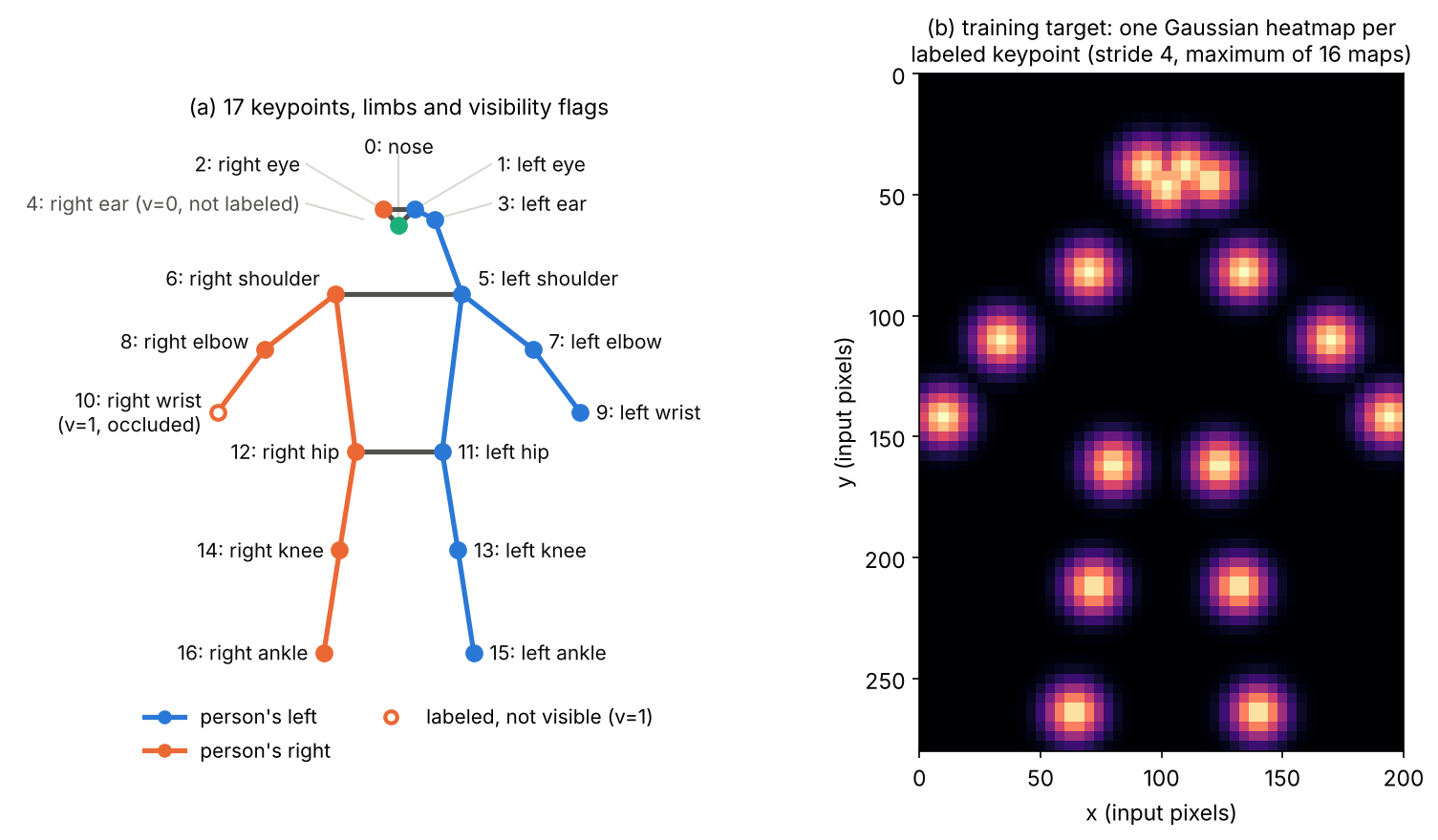
where is the image position of keypoint in pixels and is its visibility flag. The COCO keypoint format uses for “not labeled”, for “labeled but not visible” (occluded, position guessed by the annotator) and for “labeled and visible” [4]. A 3D pose replaces by a point , usually in millimetres in a camera or world frame.
The COCO person skeleton has keypoints: the nose, both eyes, ears, shoulders, elbows, wrists, hips, knees and ankles [4]. Figure 1 shows them on a synthetic stick figure. Two conventions trip up every beginner:
- Left and right are the person’s, not the viewer’s. A person facing the camera has their left shoulder on the right side of the image. Flipping an image horizontally therefore turns every left keypoint into a right one, and data augmentation must swap the labels as well as mirror the coordinates.
- Not visible is not the same as not labeled. An occluded wrist () still has a position and is still evaluated; an unlabeled keypoint () is simply ignored.
Pose estimation versus its neighbours
Four related tasks are easy to confuse:
| Task | Output | Where in this course |
|---|---|---|
| Generic keypoint detection | Corners and blobs that are easy to find again in another image, with descriptors; no semantic name | IP 12 |
| Object detection | One box, class and score per object | DLCV 03 |
| Instance segmentation | One pixel mask per object | DLCV 04 |
| Pose estimation | One set of named keypoints per object, connected by a fixed skeleton | this chapter |
The keypoints of IP 12 are chosen by the image: wherever a corner or blob happens to be. The keypoints here are chosen by the task: the left elbow must be found even when it lies on a smooth sleeve with no corner at all. That is why semantic keypoints are learned from labeled examples rather than detected by a formula.
The task comes in several flavors. Single-person 2D estimation assumes one person per input crop. Multi-person 2D estimation must also decide how many people there are and which keypoint belongs to whom. 3D estimation recovers depth. Whole-body estimation adds feet, hands and face landmarks, and mesh recovery outputs a full body surface instead of a sparse skeleton [5].
Two ways to output a keypoint
Plain version. A network can either say the numbers (“the wrist is at , ”), which is regression, or paint a picture that glows where the wrist is, which is a heatmap. For most of the deep-learning era, painting won, because convolutional networks are better at painting than at saying numbers.
Direct regression
DeepPose [6] was an early deep pose estimator built on regression. A convolutional network maps the image to a vector of numbers, the keypoint coordinates normalized by the person’s box, and is trained with a squared error,
where is the predicted and the ground-truth position of keypoint (in normalized coordinates). DeepPose refined its first guess with a cascade of further regressors applied to higher-resolution crops around each joint.
Regression is simple, fast and has no resolution limit, but the fully connected output throws away the spatial layout that convolutions are good at, and for years regression trailed heatmaps on accuracy.
Gaussian heatmaps
Tompson et al. [7] instead asked the network to output one image per keypoint type, a heatmap that is high near the keypoint and low elsewhere. The target for keypoint is a Gaussian blob centred on the true position:
where is a heatmap cell (integer coordinates), is the output stride (how many input pixels one heatmap cell covers, typically 4), is the true keypoint position in heatmap units and is the blob’s width in cells. The network is trained with a pixel-wise mean squared error between the predicted heatmaps and the targets,
where is the set of heatmap cells and is 0 for unlabeled keypoints and 1 otherwise. The stacked hourglass network uses this supervision, following Tompson et al., with pixel [8].
Why does this work so much better than regression? A heatmap matches what convolutions do: it is dense and translation-equivariant (if the person moves, the blob moves), so every output cell answers a local question, “is there a wrist here?”. It can express doubt: two plausible wrist positions become two weaker blobs, where a single regressed coordinate would land in between. And the peak height is a free confidence score for each keypoint.
The price is resolution: at stride 4 the peak can only sit on a grid of spacing 4 pixels, and maps cost far more memory than numbers. How dense prediction networks recover resolution is covered in DLCV 04; the next section shows how much the grid costs and how to get most of it back.
Decoding a heatmap: argmax, quantization error and sub-pixel refinement
Plain version. The brightest heatmap cell gives a coarse location. Neighboring responses help refine it between grid points.
The simplest decoder takes the brightest cell and maps it back to the image:
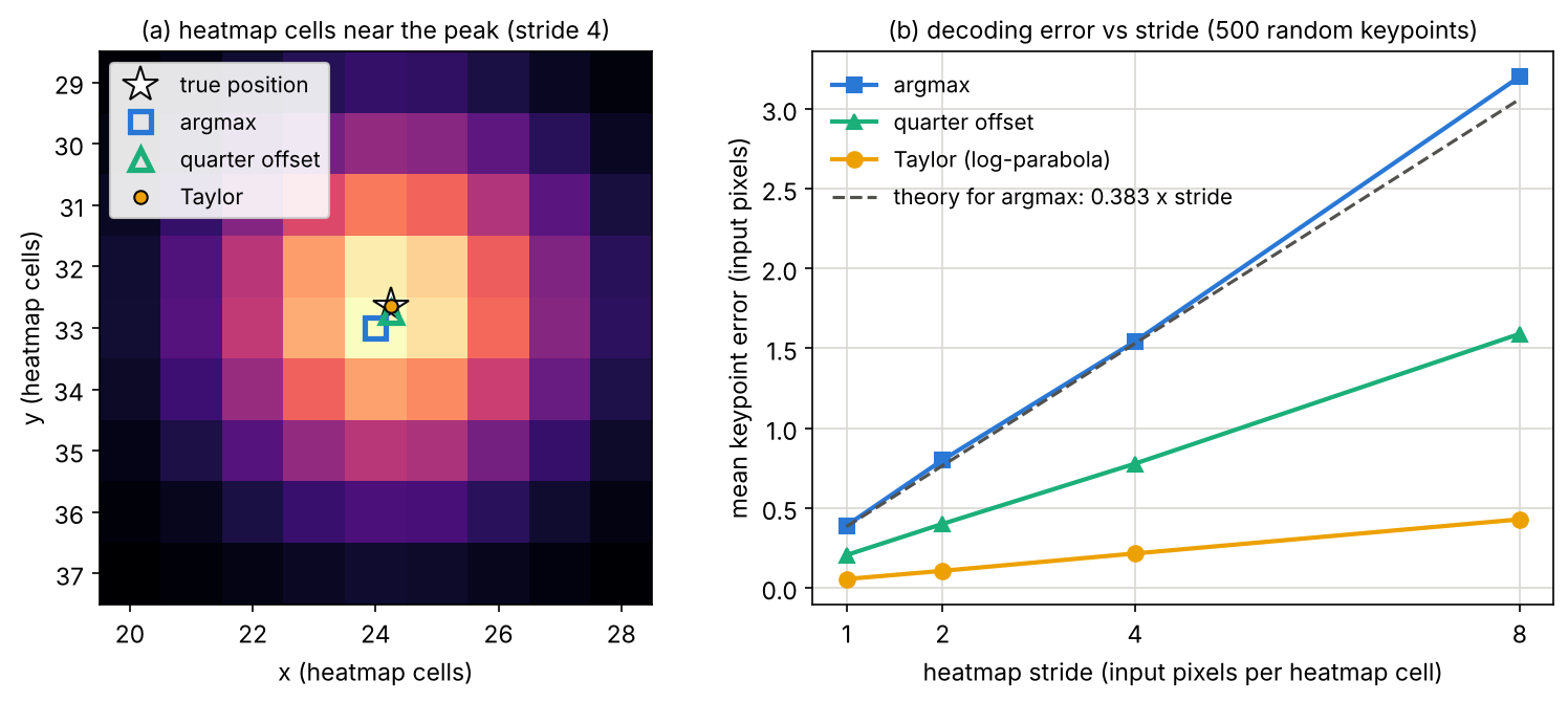
If the true position falls uniformly at random inside a cell, the error of this decoder in each axis is uniform on , and the expected Euclidean error is about (the mean distance from the centre of a unit square to a random point in it, , scaled by ). At stride 4 that is about 1.5 pixels of error before the network makes any mistake. On a person 100 pixels tall, that is enough to lose points on the strict thresholds of the OKS metric introduced later.
Three refinements are common:
- The quarter offset. Move the estimate a quarter of a cell from the peak toward its higher neighbour. The stacked hourglass paper added this to improve results at high precision thresholds [8], and SimpleBaseline uses it as standard practice [9].
- A Taylor step on the log-heatmap. The logarithm of a Gaussian is a quadratic (a parabola), so its maximum can be found exactly from the value, slope and curvature at the brightest cell: , where is the brightest cell, and and are the gradient and Hessian of there, estimated by finite differences. This is the decoding step of DARK [10]. DARK also smooths the predicted heatmap with a Gaussian before decoding, because real predictions are not perfect Gaussians, and centres the training targets on the exact (unrounded) keypoint position, as our formula for already does.
- Soft-argmax (integral regression). Treat the heatmap as a probability distribution and output its mean: , with over all cells. Sun et al. [11] showed that this turns the heatmap into a differentiable regression output, so the network can be trained end to end on the coordinates, without quantization.
DARK’s ablation makes the size of the effect concrete: for an HRNet-W32 model with a small input on COCO validation, AP was 61.2 with plain argmax, 66.9 with the quarter offset and 68.4 with its Taylor decoding [10]. The decoder alone moved AP by more than 7 points.
Optional: Sub-pixel decoding by a Taylor step (in the Supplementary notes). The derivation of the Newton step, why it is exact for a Gaussian, and the edge cases (borders, flat and multi-peaked maps).
The code encodes 500 random keypoints into heatmaps at strides 1, 2, 4 and 8, adds a little noise to imitate an imperfect prediction, and decodes them with each method. All numbers come from this synthetic run.
Code · Python · 63 lines
import numpy as np

def encode(xy, shape, stride, sigma=2.0):
    """Gaussian heatmap of size shape=(H, W) cells for a keypoint at image position xy."""
    cx, cy = xy[0] / stride, xy[1] / stride            # exact (unrounded) center in cells
    ys, xs = np.mgrid[0:shape[0], 0:shape[1]]
    return np.exp(-((xs - cx) ** 2 + (ys - cy) ** 2) / (2 * sigma ** 2))

def peak(h):
    y, x = np.unravel_index(np.argmax(h), h.shape)
    return x, y

def decode_argmax(h, stride):
    x, y = peak(h)
    return np.array([x, y], float) * stride

def decode_quarter(h, stride):
    """Move a quarter cell from the peak toward the higher neighbour on each axis."""
    x, y = peak(h)
    p = np.array([x, y], float)
    if 0 < x < h.shape[1] - 1: p[0] += 0.25 * np.sign(h[y, x + 1] - h[y, x - 1])
    if 0 < y < h.shape[0] - 1: p[1] += 0.25 * np.sign(h[y + 1, x] - h[y - 1, x])
    return p * stride

def decode_taylor(h, stride):
    """One Newton step on log h at the peak: offset = -Hessian^-1 * gradient."""
    x, y = peak(h)
    p = np.array([x, y], float)
    if 1 <= x < h.shape[1] - 1 and 1 <= y < h.shape[0] - 1:
        L = np.log(np.maximum(h[y - 1:y + 2, x - 1:x + 2], 1e-10))
        g = np.array([L[1, 2] - L[1, 0], L[2, 1] - L[0, 1]]) / 2
        hxx = L[1, 2] - 2 * L[1, 1] + L[1, 0]
        hyy = L[2, 1] - 2 * L[1, 1] + L[0, 1]
        hxy = (L[2, 2] - L[2, 0] - L[0, 2] + L[0, 0]) / 4
        Hs = np.array([[hxx, hxy], [hxy, hyy]])
        if np.linalg.det(Hs) > 0 and hxx < 0:          # a proper maximum
            p += -np.linalg.solve(Hs, g)
    return p * stride

def decode_soft(logits, stride):
    """Soft-argmax: the expected position under softmax(logits)."""
    w = np.exp(logits - logits.max()); w /= w.sum()
    ys, xs = np.mgrid[0:w.shape[0], 0:w.shape[1]]
    return np.array([(w * xs).sum(), (w * ys).sum()]) * stride

rng = np.random.default_rng(0)
W, H = 192, 256                                    # input crop size in pixels (width, height)
pts = rng.uniform([16, 16], [W - 16, H - 16], (500, 2))

def mean_error(decoder, s, noise=0.01, use_log=False):
    shape, e = (H // s, W // s), 0.0
    for xy in pts:
        h = encode(xy, shape, s)
        h = np.clip(h + rng.normal(0, noise, h.shape), 1e-6, None)   # an imperfect "prediction"
        e += np.linalg.norm(decoder(np.log(h) if use_log else h, s) - xy)
    return e / len(pts)

print("stride  argmax  quarter  taylor   (mean error in input pixels)")
for s in (1, 2, 4, 8):
    print(f"{s:6d}  {mean_error(decode_argmax, s):6.2f}  {mean_error(decode_quarter, s):7.2f}"
          f"  {mean_error(decode_taylor, s):6.2f}")
print(f"soft-argmax, stride 4: clean map {mean_error(decode_soft, 4, 0.0, True):.2f},"
      f" noisy map {mean_error(decode_soft, 4, 0.01, True):.2f}")
Output
stride  argmax  quarter  taylor   (mean error in input pixels)
     1    0.39     0.20    0.05
     2    0.80     0.40    0.11
     4    1.54     0.78    0.21
     8    3.20     1.59    0.43
soft-argmax, stride 4: clean map 0.04, noisy map 24.42
Four lessons are visible, and Figure 2 plots the first three.
- Argmax error grows linearly with the stride and follows the prediction closely (0.38, 0.77, 1.53, 3.06 for strides 1 to 8).
- The quarter offset halves it, at no cost.
- The Taylor step removes most of what remains, because the log of a Gaussian really is a parabola; what is left comes from the added noise.
- Soft-argmax is exact on a clean map but fails badly on a noisy one. With logits equal to , the softmax weights are proportional to , and a small noise floor spread over thousands of cells outweighs the narrow peak and pulls the mean toward the centre of the map. Integral regression trains the network through the soft-argmax, which pushes it to put almost no mass away from the keypoint; applied after the fact to a heatmap trained with MSE, soft-argmax is a poor decoder.
Other output representations
Two newer representations sit between heatmaps and plain regression. Coordinate classification (SimCC [12]) predicts two one-dimensional distributions per keypoint, over and over , with several bins per pixel, which cuts quantization error without a large 2D map. Likelihood-based regression (RLE [13]) keeps direct regression but learns the shape of the error distribution during training, and its paper reports regression beating heatmap methods on multi-person pose. Both are the natural outputs for the one-stage and query-based models later in this chapter.
Optional: Coordinate classification and likelihood-based regression (in the Supplementary notes). How SimCC’s bins and splitting factor work, and why the choice of regression loss is an assumption about the error distribution.
Networks for single-person heatmaps
Plain version. Precise localization needs high-resolution detail; identifying the correct joint also needs context from the body.
The input is a person crop: a box around one person, enlarged a little, padded to a fixed aspect ratio and resized to a fixed size such as (height × width). The output is heatmaps at stride 4, in this case.
- Convolutional Pose Machines (CPM) [14] stack several stages. Each stage sees the image features and the previous stage’s heatmaps (belief maps), so later stages can use the positions of other joints as context, for example “an elbow lies between a shoulder and a wrist”. Each stage is supervised (intermediate supervision), which counters vanishing gradients in a deep stack.
- Stacked hourglass networks [8] repeat a symmetric encoder–decoder (“hourglass”) module several times, with intermediate supervision after each one. Every hourglass pools down to a very coarse resolution to gather whole-body context and upsamples back with skip connections, the same encoder–decoder idea described for segmentation in DLCV 04.
- SimpleBaseline [9] showed that much of this machinery was unnecessary. It takes an ImageNet-pretrained ResNet (DLCV 02) and adds three deconvolution (transposed convolution) layers on top of its last stage to produce heatmaps for a input. Its ablation found that three deconvolution layers (heatmaps at ) beat two (at ) by 2.5 AP, a direct measurement of the resolution cost discussed above.
- HRNet [15] keeps a high-resolution branch alive through the whole network instead of recovering resolution at the end. It adds lower-resolution branches one by one, runs them in parallel and repeatedly exchanges information between all resolutions (multi-scale fusion). The heatmaps are read from the high-resolution branch, which has seen coarse context many times. Several later methods in this chapter build on HRNet: DARK reports its decoding results with HRNet models, and HigherHRNet and DEKR extend it to bottom-up pose.
- ViTPose [16] replaces the convolutional backbone by a plain, non-hierarchical vision transformer (ML 05) with patches, followed by a lightweight decoder of a few deconvolution layers (or even a single upsampling layer and a convolution). The paper scales it from 100M to 1B parameters and shows that simple design plus large pretrained transformers sets a new accuracy–throughput trade-off.
Optional: Simple Baselines (Xiao et al., 2018) (in the Paper guides). What the paper’s ablations measure and what to check when you compare its numbers with other methods.
Two training details matter for every model in this list. Data augmentation rotates, scales and flips the crops; a horizontal flip must swap the left and right keypoint channels. Flip testing runs the model on the crop and on its mirror image, swaps the channels of the mirrored output back, and averages the heatmaps; the stacked hourglass paper reports about a 1% average improvement on validation from this [8], and later models adopted it as standard practice [9].
Optional: Flip testing and left–right bookkeeping (in the Supplementary notes). The index arithmetic of mirroring a heatmap and what goes wrong when the channels are not swapped.
Many people: top-down versus bottom-up
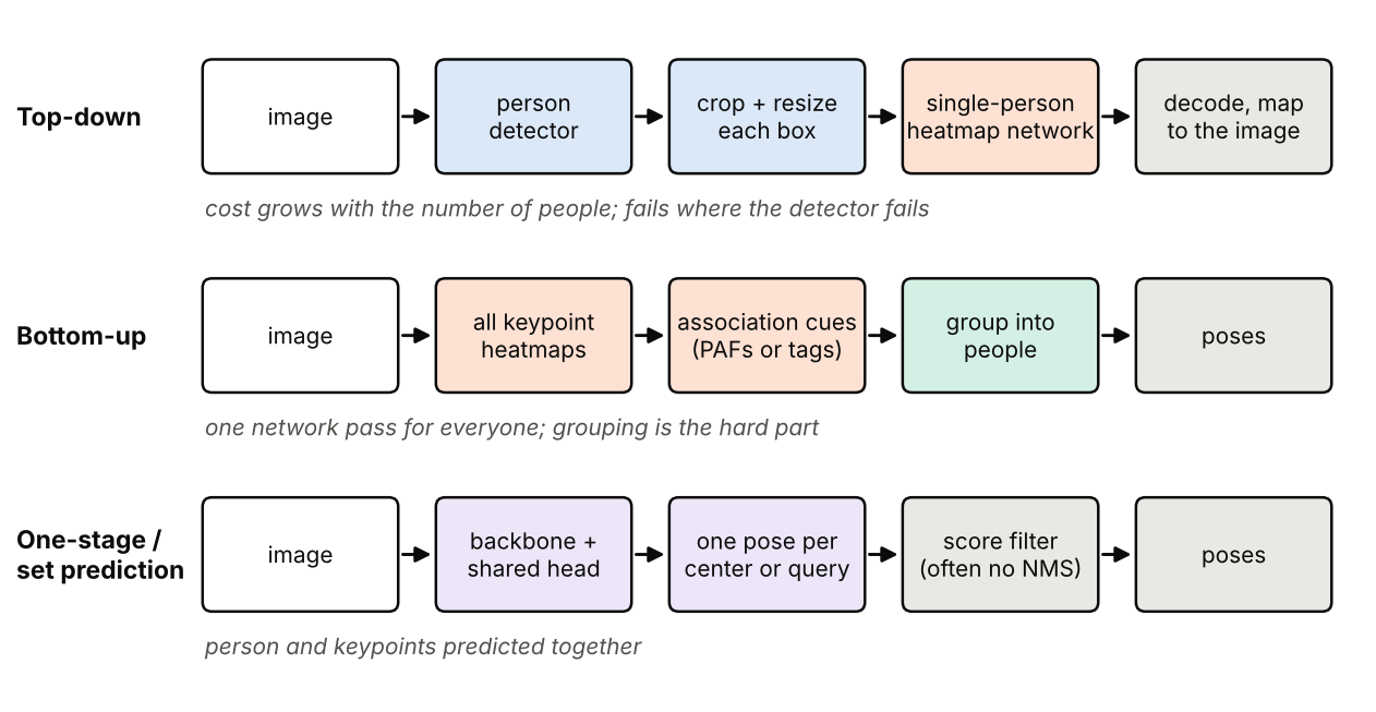
Plain version. With several people in a photo there are two orders of work. Top-down: first find each person, then find the joints inside each person’s box. Bottom-up: first find every joint in the picture, then work out which joints belong together. A third family does both at once.
Top-down: detect, then estimate
A person detector (DLCV 03) proposes boxes; each box is cropped, resized and passed to a single-person network such as SimpleBaseline, HRNet or ViTPose; the heatmaps are decoded and the keypoints mapped back to image coordinates. Mask R-CNN [17] builds the same idea into the detector: its keypoint branch predicts, inside each region of interest, masks of size , each trained as an -way softmax whose target is a single “one-hot” pixel at the keypoint (see DLCV 03 for the RoI machinery).
Top-down methods are accurate because every person is resized to the same comfortable scale before the keypoint network sees them, which helps most for small and medium-sized people [18]. Their weaknesses follow from the pipeline:
- Cost grows with the number of people, since the keypoint network runs once per box.
- They fail where the detector fails. A missed person gets no pose; NMS (DLCV 03) may delete one of two overlapping people; and a box that contains two people gives the single-person network two left wrists to choose from. The OpenPose authors measured this on a COCO validation subset: the same single-person model scored 62.7 AP with ground-truth boxes but 52.7 AP with boxes from an SSD detector [18].
Bottom-up: detect all keypoints, then group
A bottom-up model runs once on the whole image and outputs heatmaps that contain the keypoints of all people. Peaks are found with a local-maximum test, which is a per-keypoint NMS. The hard part is grouping: deciding which left elbow goes with which left wrist.
Part affinity fields (PAFs). OpenPose [18] predicts, besides the heatmaps, one 2D vector field per limb type. At a pixel on limb of person , the target is the unit vector pointing along that limb; elsewhere it is zero:
where and are the two keypoint types joined by limb (for example left elbow and left wrist), is the position of keypoint of person , and “on the limb” means within a distance (the limb width, in pixels) of the segment between them. Where limbs of several people overlap, the targets are averaged. To score a candidate connection between two detected keypoints and , OpenPose integrates the predicted field along the segment joining them:
where runs along the segment, and the integral is approximated by sampling a few evenly spaced values of . is high when the field along the segment points the same way as the segment, which happens only if the two keypoints really are the ends of one limb. Finding the best assignment for all limbs at once is NP-hard, so OpenPose relaxes it: it keeps only the edges of a tree skeleton and solves one bipartite matching per limb type, for example with the Hungarian algorithm (see DLCV 07), then joins limbs that share keypoints into people.
Optional: OpenPose: part affinity fields (Cao et al., 2017) (in the Paper guides). The two-branch architecture, the greedy parse, and how to read the paper’s top-down versus bottom-up comparison.
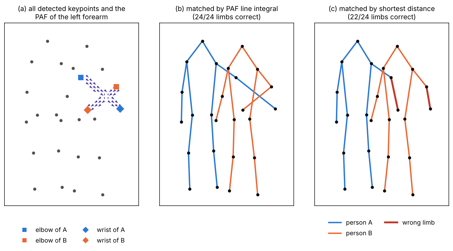
The code builds the ground-truth PAFs of two people standing side by side whose left forearms cross, adds small noise to the keypoint positions, and groups the keypoints limb by limb, once with the PAF score and once with plain distance (the shortest total limb length). The coordinates are synthetic.
Code · Python · 55 lines
import numpy as np
from scipy.optimize import linear_sum_assignment

# 13 body keypoints and the 12 limbs of a tree that connects them
J = ["nose", "l_sho", "r_sho", "l_elb", "r_elb", "l_wri", "r_wri",
     "l_hip", "r_hip", "l_knee", "r_knee", "l_ank", "r_ank"]
LIMBS = [(0, 1), (0, 2), (1, 3), (3, 5), (2, 4), (4, 6),
         (1, 7), (2, 8), (7, 9), (9, 11), (8, 10), (10, 12)]

# two people side by side; their left forearms cross (synthetic coordinates)
A = np.array([[40, 20], [52, 38], [28, 38], [70, 50], [24, 62], [100, 74], [22, 86],
              [48, 80], [32, 80], [50, 110], [30, 110], [52, 140], [28, 140]], float)
B = np.array([[72, 24], [84, 42], [62, 42], [98, 58], [56, 64], [74, 76], [52, 86],
              [80, 84], [66, 84], [82, 114], [64, 114], [84, 144], [62, 144]], float)
people = [A, B]
H, W, width = 160, 120, 3.0

def render_paf(c):
    """Ground-truth part affinity field of limb c: unit vectors near each person's limb."""
    ys, xs = np.mgrid[0:H, 0:W]
    field, count = np.zeros((H, W, 2)), np.zeros((H, W))
    for P in people:
        a, b = P[LIMBS[c][0]], P[LIMBS[c][1]]
        v = (b - a) / np.linalg.norm(b - a)
        along = (xs - a[0]) * v[0] + (ys - a[1]) * v[1]
        across = np.abs(-(xs - a[0]) * v[1] + (ys - a[1]) * v[0])
        on = (along >= 0) & (along <= np.linalg.norm(b - a)) & (across <= width)
        field[on] += v; count[on] += 1
    return field / np.maximum(count, 1)[..., None]          # average where limbs overlap

def limb_score(field, p, q, n=10):
    """Line integral of the field along the segment p -> q, approximated by n samples."""
    d = (q - p) / np.linalg.norm(q - p)
    u = np.linspace(0, 1, n)[:, None]
    pts = np.round(p + u * (q - p)).astype(int)
    return np.mean(field[pts[:, 1], pts[:, 0]] @ d)

rng = np.random.default_rng(0)
cands = [np.stack([A[j], B[j]]) + rng.normal(0, 1.0, (2, 2)) for j in range(13)]  # detections

ok_paf = ok_near = 0
for c, (j1, j2) in enumerate(LIMBS):
    field = render_paf(c)
    S = np.array([[limb_score(field, p, q) for q in cands[j2]] for p in cands[j1]])
    D = np.linalg.norm(cands[j1][:, None] - cands[j2][None], axis=2)
    if (j1, j2) == (3, 5):                                    # the crossing forearms
        print("left elbow -> left wrist, PAF scores (rows: elbows A, B; cols: wrists A, B)")
        print(np.round(S, 2))
        print("distances in pixels"); print(np.round(D, 1))
    r, k = linear_sum_assignment(-S)                          # maximize total affinity
    ok_paf += np.sum(k == r)                                  # candidate i belongs to person i
    r, k = linear_sum_assignment(D)                           # baseline: shortest total length
    ok_near += np.sum(k == r)
print(f"correct limbs with PAF scores:     {ok_paf}/{2 * len(LIMBS)}")
print(f"correct limbs with distance only:  {ok_near}/{2 * len(LIMBS)}")
Output
left elbow -> left wrist, PAF scores (rows: elbows A, B; cols: wrists A, B)
[[0.67 0.04]
 [0.29 0.78]]
distances in pixels
[[41.1 27.2]
 [18.4 30.2]]
correct limbs with PAF scores:     24/24
correct limbs with distance only:  22/24
The printed matrices show the failure of geometry alone. Each elbow is closer to the other person’s wrist (27.2 and 18.4 pixels) than to its own (41.1 and 30.2), so matching by distance connects both forearms wrongly. The PAF score is high only along the true limbs (0.67 and 0.78), because the field there points along the segment; along the wrong pairings it is low. Figure 4 draws both results. Note that the PAF here is the ground truth; a trained network predicts a blurrier field, and the method’s accuracy depends on how well it does so.
Associative embedding. Newell et al. [19] avoid limb fields altogether. Alongside each keypoint heatmap the network outputs a tag map: one real number per pixel. Training pushes the tags of one person’s keypoints to be equal and the tags of different people to be different. With the tag of keypoint type at pixel , the ground-truth position of keypoint of person , people and the mean tag of person , the grouping loss is
where the first term pulls each person’s tags toward their mean and the second pushes the means of different people apart, with a penalty that fades as the distance between them grows ( sets how far apart is “far enough”). The absolute tag values do not matter, only their differences. At test time, keypoints are added to people joint by joint, matching tags that are close and detections that are confident. CornerNet borrowed exactly this idea to pair box corners (DLCV 03).
Scale. Bottom-up methods see all people at the image’s own scale, so small people get few heatmap cells; OpenPose was less accurate than top-down methods on medium-sized people for this reason [18]. HigherHRNet [20] adds higher-resolution heatmaps (HRNet’s output upsampled by a transposed convolution) and supervises and aggregates several resolutions; its paper reports results above all top-down methods on the CrowdPose test set, where boxes are unreliable. DEKR [21] returns to dense regression, with one branch per keypoint whose adaptive convolutions focus on that keypoint’s region, and reports better results than detection-and-grouping methods on COCO and CrowdPose.
One-stage and set-prediction pose
A third family predicts a whole pose per person directly, without a separate grouping step.
- Center-based. CenterNet (“Objects as Points”) [22] detects each person as a centre point on a heatmap and regresses the offsets from the centre to the keypoints; it then snaps each regressed keypoint to the nearest peak of a separate keypoint heatmap, so the centre acts as the grouping cue.
- Real-time dense heads. RTMO [23] puts a pose head into a YOLO-style one-stage detector and represents each keypoint with a pair of one-dimensional heatmaps (coordinate classification), aiming at top-down accuracy at one-stage speed.
- Set prediction. Transformer detectors in the DETR style (DLCV 03) output a fixed set of queries matched one-to-one to the ground truth, so no NMS or grouping is needed. ED-Pose [24] applies this to pose with two explicit box-detection stages: a human decoder detects people, and a human-to-keypoint decoder treats each keypoint as a small box to detect. Trained with an L1 regression loss and no heatmaps, it reports results above heatmap-based top-down methods with the same backbone on COCO.
Choosing a pipeline
| Top-down | Bottom-up | One-stage / set prediction | |
|---|---|---|---|
| Main step | Detect people, then estimate each | Detect all keypoints, then group | Predict each person’s pose directly |
| Cost vs number of people | Grows linearly | Nearly constant network cost; grouping grows | Nearly constant |
| Small people | Good (each crop is resized) | Harder (one image scale for all) | Depends on the feature pyramid |
| Crowds and overlap | Boxes overlap; NMS can remove people | Grouping can mix people | Queries or centres can collide |
| Typical use | High accuracy when people are few and well separated | Many people at once; real-time systems | End-to-end training; real-time |
Measuring pose accuracy
Plain version. A predicted keypoint is “good” if it is close to the true one, but “close” must depend on the size of the person and on the keypoint: being 5 pixels off on a tiny person’s nose is a big mistake; 5 pixels off on a large person’s hip is not.
PCK and PCKh
The percentage of correct keypoints (PCK) counts a predicted keypoint as correct if it lies within a threshold distance of the ground truth, where the threshold is a fraction of the person’s size. Yang and Ramanan used a fraction of the person’s bounding-box size [25]. MPII’s PCKh [26] uses 50% of the head segment length instead, because head size does not change when the person bends or stretches. Formally,
where indexes people, keypoints, is the head segment length of person , is the fraction ( for the standard PCKh), and are 1 when their condition holds and 0 otherwise, and only labeled keypoints count. PCK assumes the person has been found; it does not penalize missed or invented people, which is why multi-person benchmarks use an AP-style metric.
Object keypoint similarity and keypoint AP
COCO’s metric mirrors box detection (DLCV 03). In box AP, a detection is matched to a ground-truth box if their IoU passes a threshold. In keypoint AP, a predicted pose is matched to a ground-truth person if their object keypoint similarity (OKS) passes a threshold [4]:
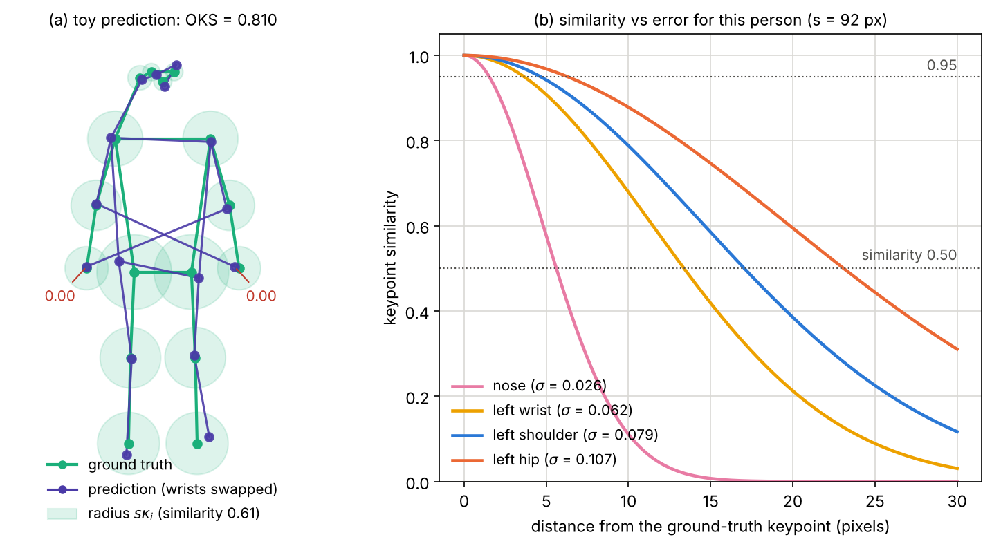
where runs over the keypoints, is the Euclidean distance between the predicted and ground-truth keypoint , is the ground-truth visibility flag, is the object scale, defined as the square root of the person’s segmentation area, and is a per-keypoint constant. Each term is an unnormalized Gaussian of the error with standard deviation , so it is 1 for a perfect keypoint and falls toward 0 as the error grows; OKS averages it over the labeled keypoints. The predicted visibility flags are not used.
Where the constants come from. COCO had 5,000 validation images annotated twice and measured, for each keypoint type, how much human annotators disagree relative to the person’s scale, . It then set [4]. The values of are 0.026 for the nose, 0.025 for the eyes, 0.035 for the ears, 0.079 for the shoulders, 0.072 for the elbows, 0.062 for the wrists, 0.107 for the hips, 0.087 for the knees and 0.089 for the ankles [4], [27]. Eyes are easy to place exactly; hips, hidden under clothing, are not, so the metric is more forgiving for hips. With , errors of one, two and three annotator standard deviations give similarities of , and , and human annotators reach a median OKS of about 0.91 against each other [4].
From OKS to AP. The rest is the AP of DLCV 03: rank all predicted poses by their person-level score, match each to the unmatched ground-truth person with the highest OKS, and compute AP at OKS thresholds . The primary metric, AP, averages these ten values. Companion metrics are , , for medium people (area between and ) and for large ones (area above ), plus the matching AR values. At most 20 poses per image are scored, and small people have no keypoint labels [4].
Optional: Inside OKS: unlabeled people, crowds and the scale s (in the Supplementary notes). How the evaluation code treats people without labeled keypoints, why every person counts equally, and what means for a person who is partly hidden.
The code computes OKS with COCO’s constants for a synthetic person about 200 pixels tall.
Code · Python · 34 lines
import numpy as np

NAMES = ["nose", "l_eye", "r_eye", "l_ear", "r_ear", "l_shoulder", "r_shoulder",
         "l_elbow", "r_elbow", "l_wrist", "r_wrist", "l_hip", "r_hip",
         "l_knee", "r_knee", "l_ankle", "r_ankle"]
SIGMAS = np.array([.26, .25, .25, .35, .35, .79, .79, .72, .72, .62, .62,
                   1.07, 1.07, .87, .87, .89, .89]) / 10.0       # COCO per-keypoint constants

def oks(pred, gt, vis, area):
    """pred, gt: (17, 2) pixel coordinates; vis: (17,) COCO flags; area: segment area (s^2)."""
    d2 = ((pred - gt) ** 2).sum(1)
    kappa = 2 * SIGMAS
    ks = np.exp(-d2 / (2 * area * kappa ** 2))                 # per-keypoint similarity
    labeled = vis > 0
    return ks[labeled].mean(), ks

# a standing person about 200 px tall, facing the camera (synthetic coordinates)
gt = np.array([[100, 30], [106, 25], [94, 25], [112, 28], [88, 28], [125, 60], [75, 60],
               [135, 95], [65, 95], [140, 128], [60, 128], [115, 130], [85, 130],
               [117, 175], [83, 175], [118, 220], [82, 220]], float)
vis = np.full(17, 2); vis[3] = 0                                # left ear not labeled
area = 0.6 * (70 * 200)                                         # segment area: ~60% of its box

rng = np.random.default_rng(1)
jitter = gt + rng.normal(0, 3, gt.shape)                        # every keypoint off by ~3 px per axis
flipped = jitter.copy(); flipped[[9, 10]] = flipped[[10, 9]]    # left/right wrists swapped
print(f"perfect          OKS = {oks(gt, gt, vis, area)[0]:.3f}")
print(f"3 px jitter      OKS = {oks(jitter, gt, vis, area)[0]:.3f}")
print(f"+ wrists swapped OKS = {oks(flipped, gt, vis, area)[0]:.3f}")

# the same 5-pixel error costs very different amounts on different keypoints
for k in (0, 5, 11):
    p = gt.copy(); p[k, 0] += 5
    print(f"5 px error on {NAMES[k]:10s}: similarity {oks(p, gt, vis, area)[1][k]:.3f}")
Output
perfect          OKS = 1.000
3 px jitter      OKS = 0.933
+ wrists swapped OKS = 0.810
5 px error on nose      : similarity 0.577
5 px error on l_shoulder: similarity 0.942
5 px error on l_hip     : similarity 0.968
Three lessons follow from this synthetic example. Small jitter everywhere costs little (0.933). A single left–right swap of the wrists sets both wrist similarities to essentially zero and drops OKS to 0.810: this pose still counts as correct at thresholds up to 0.80 but fails at 0.85 and above, so it loses about a third of the ten AP thresholds. And the same 5-pixel error costs 0.42 of similarity on the nose but only 0.03 on a hip. Figure 5 shows the tolerance radius of each keypoint and the similarity curves.
Metrics for 3D pose
For 3D pose, the standard metric is the mean per-joint position error (MPJPE), the average Euclidean distance between predicted and ground-truth 3D joints,
reported in millimetres and averaged over all test frames, where and are the predicted and true 3D positions of joint . Two protocols are common on Human3.6M: errors after aligning the root (central hip) joints of prediction and ground truth, called Protocol #1, and errors after an additional rigid alignment of the predicted skeleton to the ground truth, called Protocol #2 [28]; the second metric is also known as PA-MPJPE or reconstruction error [2]. The second hides errors in global rotation and scale, so the two numbers must never be compared with each other.
What the numbers do not tell you
Like box AP, keypoint AP mixes several kinds of error. Ronchi and Perona [29] split keypoint localization errors into four types: jitter (near the right keypoint but outside the human error margin), inversion (at the person’s own left–right twin or another of their keypoints), swap (at a keypoint of a different person) and miss (near no keypoint). They found that errors depend most on the number of visible keypoints and on clutter from nearby people. Even COCO’s doubly annotated data contain 1–2% outliers, mostly left–right confusions or the wrong person labeled [4]. Diagnose models by error type, not only by AP.
Datasets and benchmarks
Plain version. A handful of datasets defined what “good” means: COCO for many people in everyday photos, MPII for a wide range of activities, CrowdPose for heavy overlap, Human3.6M for 3D, and newer sets for whole bodies, video and animals.
| Dataset | Content (from the papers or official pages) | Metric | Why it matters |
|---|---|---|---|
| COCO keypoints [30], [4] | 17 body keypoints on people in everyday photos; small people unlabeled | OKS AP | The main multi-person benchmark |
| MPII Human Pose [26] | 40,522 annotated people in images from YouTube videos, collected with queries for more than 800 activities | PCKh | Diverse activities; single- and multi-person tracks |
| CrowdPose [31] | 20,000 images, about 80,000 people, 14 keypoints, selected for a uniform spread of crowding | OKS AP | Crowded scenes |
| COCO-WholeBody [32] | 133 landmarks per person: 68 face, 42 hand, 23 body and feet | OKS AP | Face, hands and feet together |
| PoseTrack [33] | Videos with person tracks and articulated poses | AP, MOTA | Pose estimation and tracking in video |
| Human3.6M [34] | 3.6 million 3D poses of 11 actors in 17 scenarios, recorded by 4 calibrated cameras with motion capture | MPJPE | The most widely used 3D benchmark |
| AP-10K [35] | 10,015 images of 54 mammal species from 23 families, annotated in COCO style | AP | Animal pose and cross-species generalization |
CrowdPose deserves a closer look because it defines crowding precisely. For person , let be the number of its own joints inside its box and the number of other people’s joints inside the same box; the Crowd Index of an image with people is [31]. Common datasets are dominated by uncrowded images; CrowdPose was selected so that this index is spread nearly uniformly between 0 and 1, and its authors found the accuracy of strong models to be about 20 AP lower on crowded images than on uncrowded ones [31].
Two cautions apply when reading results. Human3.6M is an indoor dataset with a few actors [2], [34], so low MPJPE there does not imply good results on outdoor video. And on COCO, results depend on the person detector used by top-down methods (see the Simple Baselines guide), on input resolution and on extra training data, so compare numbers only under the same settings.
Beyond the human body
Plain version. Nothing in a heatmap network is specific to people. Change the list of keypoints and the training data, and the same machinery finds the corners of a face, the joints of a hand, or the paws of a dog.
- Whole body. COCO-WholeBody [32] adds feet, hands and dense face landmarks to the body keypoints, which creates a huge range of scales inside one person; its baseline model, ZoomNet, is built around the body’s hierarchical structure to handle this. The journal version of OpenPose [36] added foot keypoints.
- Animals. AP-10K [35] benchmarks pose across 54 mammal species and tests generalization to unseen animal families. In neuroscience, DeepLabCut [1] uses transfer learning from a pretrained network to track user-defined body parts of mice and flies from about 200 labeled frames in its experiments, replacing reflective markers.
- Objects. The same formulation works for any category with consistent landmarks, such as the wheels and lights of cars, provided the keypoints are defined consistently and the category’s left–right symmetries are handled like the body’s.
From 2D to 3D pose
Plain version. A photo flattens the world: from one image, a hand pointing at the camera and a hand held at the hip can look almost the same. There are three ways to get the depth back: guess it from experience (lifting), measure it with two or more cameras (triangulation), or fit a model of the human body that only allows realistic shapes.
Lifting 2D keypoints
Martinez et al. [28] showed that a surprisingly large part of monocular 3D pose estimation is solved once the 2D keypoints are known. Their model takes the coordinates of a detected 2D pose and maps them with a simple fully connected network (linear layers with batch normalization, dropout and residual connections) to coordinates. Trained on Human3.6M, it beat the previous best methods by a large margin when given ground-truth 2D keypoints, which suggests that much of the remaining difficulty lies in the 2D detection rather than in the lifting. Lifting is also ambiguous: several 3D poses project to the same 2D pose, and a network with a single output can return only one of them.
VideoPose3D [37] lifts a whole sequence of 2D poses with dilated temporal convolutions, so motion over neighbouring frames helps resolve depth and jitter. It also introduced back-projection, a semi-supervised loss that estimates 3D poses for unlabeled video and requires them to project back onto the detected 2D keypoints.
Multi-view triangulation
With two or more calibrated cameras, depth is no longer a guess. Each camera’s 2D keypoint defines a ray in space, and the 3D joint is the point where the rays (almost) meet. The geometry is the triangulation of DLCV 11, applied joint by joint: the camera matrices are the pinhole models of that chapter, and the linear (DLT) solution is derived in its Supplementary notes. Learnable triangulation [38] makes this step part of the network: it weights each view by a confidence predicted from the image, so that a view in which the joint is occluded contributes less, and its second variant aggregates 2D features from all views into a 3D volume refined by 3D convolutions.
The code projects a synthetic 13-joint skeleton, standing 4 m from two converging cameras, into both images, adds 2-pixel noise to the 2D keypoints, triangulates every joint with the DLT and reports MPJPE for three distances between the cameras (the baseline). The numbers come from this synthetic run, without root alignment.
Code · Python · 38 lines
import numpy as np

def camera(K, angle_deg, center):
    """3x4 projection P = K [R | t] for a camera at `center` rotated about the y axis."""
    a = np.deg2rad(angle_deg)
    R = np.array([[np.cos(a), 0, -np.sin(a)], [0, 1, 0], [np.sin(a), 0, np.cos(a)]])
    return K @ np.hstack([R, -R @ center[:, None]])

def project(P, X):
    x = (P @ np.hstack([X, np.ones((len(X), 1))]).T).T
    return x[:, :2] / x[:, 2:]

def triangulate(Ps, xs):
    """Linear (DLT) triangulation of one point seen in several views."""
    A = []
    for P, (u, v) in zip(Ps, xs):
        A += [u * P[2] - P[0], v * P[2] - P[1]]
    X = np.linalg.svd(np.array(A))[2][-1]
    return X[:3] / X[3]

# a 13-joint 3D skeleton in millimetres, standing 4 m in front of the cameras (synthetic)
skel = np.array([[0, -1650, 0], [170, -1400, 0], [-170, -1400, 0], [250, -1120, 50], [-250, -1120, 50],
                 [280, -860, 120], [-280, -860, 120], [100, -900, 0], [-100, -900, 0],
                 [110, -480, 30], [-110, -480, 30], [110, -60, 0], [-110, -60, 0]], float)
skel += [0, 900, 4000]
K = np.array([[1000, 0, 640], [0, 1000, 360], [0, 0, 1]], float)

rng = np.random.default_rng(0)
for baseline in (200, 1000, 3000):                          # distance between the cameras (mm)
    half = baseline / 2
    Ps = [camera(K, np.degrees(np.arctan2(half, 4000)), np.array([-half, 0, 0.])),
          camera(K, -np.degrees(np.arctan2(half, 4000)), np.array([half, 0, 0.]))]
    errs = []
    for trial in range(200):                                  # 2D detections with 2 px noise
        obs = [project(P, skel) + rng.normal(0, 2.0, (13, 2)) for P in Ps]
        est = np.array([triangulate(Ps, [o[j] for o in obs]) for j in range(13)])
        errs.append(np.linalg.norm(est - skel, axis=1).mean())   # MPJPE of this trial
    print(f"baseline {baseline:4d} mm: MPJPE = {np.mean(errs):6.1f} mm")
Output
baseline  200 mm: MPJPE =  183.7 mm
baseline 1000 mm: MPJPE =   37.9 mm
baseline 3000 mm: MPJPE =   17.4 mm
With cameras 20 cm apart, a 2-pixel image error becomes about 18 cm in 3D, almost all of it in depth (a per-axis check of the same run gives 182 mm in depth against 9 and 18 mm across): the rays are nearly parallel, so a small shift moves their crossing point far along them. A wider baseline makes the rays cross at a larger angle and cuts the error by a factor of ten.
Parametric body models and mesh recovery
A skeleton says nothing about body shape, and nothing stops a lifting network from predicting a forearm that changes length from frame to frame. Parametric body models fix both problems by describing a body with a small set of parameters. The most widely used is SMPL [39]. It starts from a template mesh with vertices and a skeleton with joints, and generates a posed body as
where are shape parameters (coefficients of the main modes of body-shape variation), are pose parameters (an axis–angle rotation for each joint relative to its parent, plus the global orientation: numbers), is the template mesh, and are vertex offsets that model identity and pose-dependent deformations such as bulging muscles, are the joint locations regressed from the shaped mesh, are the blend weights and is a standard blend-skinning function that rotates each vertex around the joints. Keypoints are read off the mesh, so a fitted SMPL body always has consistent bone lengths.
Human mesh recovery (HMR) [40] regresses SMPL parameters and a camera directly from an image. Its main loss is the reprojection error of the model’s joints against 2D keypoint labels, which allows training on in-the-wild images; an adversarial prior trained on real 3D bodies rejects implausible parameters. HMR 2.0, part of 4DHumans [41], makes the network fully transformer-based and tracks the reconstructed people through occlusions in video.
Optional: SMPL in more detail (in the Supplementary notes). What each term of the model does, how joints and keypoints are obtained from the mesh, and why the pose blend shapes vanish in the rest pose.
Failure modes and practical advice
Plain version. Pose models fail where people would hesitate too: hidden joints, tangled people, mirror-image confusion, bodies cut off by the frame, poses rarely seen in training, and blur.
- Occlusion. An occluded joint () is labeled but not shown, so the network must infer it from context; self-occlusion makes legs especially prone to left–right confusion [29].
- Crowds. Overlapping people break detectors, confuse grouping and cause swap errors [29]; accuracy falls as the Crowd Index rises [31].
- Left–right flips. Front and back views look alike, so a model can mirror a limb or a whole person (an inversion); a forgotten channel swap in flip augmentation causes the same error systematically.
- Truncation. Joints outside the frame are unlabeled or guessed, and crops of a partial person are poorly centred.
- Unusual poses. Gymnastics, dancing or lying people are rare in training data; HMR 2.0’s authors single them out as a case where earlier methods struggled [41].
- Motion blur, low resolution and domain shift. Fast limbs smear, small people have few pixels per limb, and models trained on adult photos transfer poorly to infants or artwork [2].
Practical advice that follows from this chapter: use an unbiased encoder and a sub-pixel decoder; check that flipping swaps left and right channels; report the detector and input size with top-down results; evaluate crowded and uncrowded images separately; break errors down by type; and in video, smooth or track keypoints over time. Tracking-by-detection with the association methods of DLCV 07 carries over directly: SimpleBaseline, for example, propagates poses to the next frame with optical flow and matches them with an OKS-based similarity [9], and PoseTrack provides the benchmark [33]. Following individual surface points instead of named joints is the point-tracking problem of DLCV 07.
Modern view
What the surveys say
Zheng et al. [2] review more than 250 deep-learning papers on 2D and 3D pose since 2014, organized as in this chapter: regression versus heatmaps, top-down versus bottom-up, and for 3D, lifting, mesh recovery and multi-view methods. Their future directions include domain adaptation, human–scene constraints and metrics for temporal smoothness.
Chen et al. [3] organize monocular methods into four tasks (2D or 3D, single- or multi-person), list the design tricks that proved effective (multi-stage structures, intermediate supervision, multi-scale fusion, body-structure constraints) and name occlusion and crowds as the main unresolved challenges.
Tian et al. [5] survey monocular 3D mesh recovery with body models, contrasting optimization-based fitting with regression networks, and point to the lack of in-the-wild 3D labels as the central difficulty.
Optional: Guide to the Modern view surveys (in the Paper guides). What each survey covers, how it is organized and how to use it as a map.
The state of the art, 2023–2026
- Scaled transformers for top-down pose. ViTPose [16] showed that plain vision transformers with simple decoders scale well (from 100M to 1B parameters in the paper), and its largest model set a new state of the art on the COCO keypoint benchmark at publication.
- Human-centric foundation models. Sapiens [42] pretrains vision transformers from 0.3 to 2 billion parameters on over 300 million images of humans with self-supervision, then fine-tunes them for 2D pose, body-part segmentation, depth and surface normals; its authors report that this human-specific pretraining improves all four tasks at the same compute budget.
- Real-time systems. RTMPose [43] (top-down, coordinate classification, engineered for CPU, GPU and mobile deployment) and RTMO [23] (one-stage) target the latency budgets of applications rather than leaderboard peaks.
- End-to-end multi-person models. Query-based models such as ED-Pose [24] remove NMS, grouping and heatmaps; ED-Pose reports higher COCO accuracy than heatmap-based top-down methods with the same backbone.
- 3D humans in video. Transformer mesh recovery such as HMR 2.0 [41] reconstructs and tracks full 3D bodies from monocular video, moving the field from sparse skeletons toward complete body surfaces.
Open problems
- Crowds and heavy occlusion remain the largest accuracy gap [31], [3].
- In-the-wild 3D. Accurate 3D labels are scarce outside the lab [5], and the most widely used 3D benchmark, Human3.6M, is an indoor dataset [2], so monocular 3D methods are trained and tested far from where they are used.
- Temporal consistency. Per-frame metrics such as MPJPE do not measure jitter or physical plausibility over time [2].
- Generalization across domains and species: infants, artwork, unusual viewpoints and unseen animal families [2], [35].
- Evaluation. OKS constants were measured from annotator disagreement on COCO people [4] and do not transfer automatically to other keypoint sets, and AP hides error types such as inversions and swaps [29].
Key takeaways
- Keep keypoint names, left/right conventions and visibility labels consistent.
- Heatmap resolution and decoding affect localization; the brightest cell alone loses sub-pixel information.
- Precise joints require both fine spatial features and enough context to identify the body part.
- Top-down methods inherit detector errors and per-person cost; bottom-up methods require grouping.
- State each metric’s scale normalization, visibility rules and coordinate convention.
- 3D lifting is ambiguous; triangulation needs calibration, and body models impose shape assumptions. Inspect errors by type.
Exercises
- Quantization by hand. A wrist lies at pixels in a crop, and the heatmap stride is 4. Which heatmap column holds the peak? What does argmax decoding return, and what is its error? What does the quarter offset return? What would an exact Taylor step on a noise-free Gaussian return?
Hint
In heatmap units the wrist is at , so the peak is in column 25 and argmax returns pixels, an error of 1.3 pixels. The right neighbour (column 26) is closer to 25.325 than the left one, so the quarter offset moves to 25.25, which maps to 101.0 pixels (error 0.3). On a noise-free Gaussian, the log-heatmap is an exact parabola, so the Taylor step returns 25.325, that is 101.3 pixels.
- OKS by hand. A person has segmentation area pixels², so . A predicted knee is 10 pixels from the ground truth. Compute its keypoint similarity with COCO’s constant. Repeat for a nose 10 pixels off. Which error would you rather make, and why does COCO treat them so differently?
Hint
Knee: , , similarity . Nose: , , similarity . Annotators place noses about three times more consistently than knees, and COCO scales the tolerance by that disagreement.
- When does top-down become too slow? A person detector takes 20 ms per image and a single-person network takes 5 ms per crop. A bottom-up network takes 40 ms per image plus 1 ms of grouping per person. For how many people per image is bottom-up faster? Name two reasons, other than speed, to prefer one pipeline in a crowded train station.
Hint
Top-down costs ms and bottom-up ms, so bottom-up is faster when , that is for more than 5 people. In a crowded station, top-down suffers from overlapping boxes and NMS removing people, but handles small distant people better because each crop is resized; bottom-up has a constant network cost but must group heavily overlapping limbs, and small people get few heatmap cells.
- Break the part affinity field. In the grouping code, move person B so that its left forearm lies on the same line as person A’s left forearm and overlaps it (one person standing behind the other). What happens to the PAF scores of the two correct and the two wrong pairings, and why? What extra cue could resolve the case?
Hint
Where the two limbs overlap, the target field is the average of two identical unit vectors, so it points along the shared line. Every candidate segment between an elbow and a wrist on that line, correct or not, is aligned with the field and gets a similar score, so the matching becomes ambiguous. Cues that can help: the lengths of the limbs relative to the rest of each body, tags as in associative embedding, the other limbs of each person (a global rather than per-limb parse), or temporal continuity in video.
- A swap the cameras cannot see. Change the triangulation code so that both cameras aim at the centre of the skeleton, and in the second camera exchange the 2D positions of the left and right knees (an inversion error of the 2D detector). Triangulate the left knee and compute its mean reprojection error in the two views, with and without the swap. Then move the second camera 1 m above the first instead of beside it and repeat. Explain the difference.
Hint
In our run of this experiment, with the cameras side by side the reprojection error is about 1 pixel with or without the swap, yet the swapped knee lands more than half a metre from the truth. The two knees are at nearly the same height, and with a horizontal baseline the epipolar lines are nearly horizontal, so swapping the knees moves the observation along its epipolar line: the two rays still meet, just at the wrong depth. With the second camera above the first, the epipolar lines become nearly vertical, the swap moves the observation off its line, and the reprojection error jumps to tens of pixels, which flags the error. Camera layouts for multi-view pose should therefore not place all cameras along one horizontal line.
- Forgetting the channel swap. You run flip testing but forget to swap the left and right channels of the mirrored heatmaps before averaging. Describe what the averaged left-wrist heatmap looks like for a person facing the camera with arms spread, and what argmax decoding returns.
Hint
Think about what the network sees in the mirrored image: a person facing the camera, so it labels the wrist on the image’s right as “left wrist”. That wrist is the person’s right wrist, mirrored. Flipping the map back without swapping channels therefore puts a blob on the true right wrist in the left-wrist channel. The average has two half-height blobs, one on each wrist, and argmax picks whichever is slightly higher, so roughly half the time the left wrist is reported on the right wrist: an inversion error.
References
- A. Mathis, P. Mamidanna, K. M. Cury, T. Abe, V. N. Murthy, M. W. Mathis and M. Bethge, “DeepLabCut: Markerless pose estimation of user-defined body parts with deep learning,” Nature Neuroscience, vol. 21, no. 9, 2018. doi · arXiv
- C. Zheng, W. Wu, C. Chen, T. Yang, S. Zhu, J. Shen, N. Kehtarnavaz and M. Shah, “Deep learning-based human pose estimation: A survey,” ACM Computing Surveys, vol. 56, no. 1, 2024. doi · arXiv
- Y. Chen, Y. Tian and M. He, “Monocular human pose estimation: A survey of deep learning-based methods,” Computer Vision and Image Understanding, vol. 192, 102897, 2020. doi · arXiv
- COCO Consortium, “Keypoint evaluation,” COCO dataset official documentation (accessed 2026-11-01). cocodataset.org
- Y. Tian, H. Zhang, Y. Liu and L. Wang, “Recovering 3D human mesh from monocular images: A survey,” IEEE Transactions on Pattern Analysis and Machine Intelligence, vol. 45, no. 12, 2023. doi · arXiv
- A. Toshev and C. Szegedy, “DeepPose: Human pose estimation via deep neural networks,” in Proc. IEEE Conference on Computer Vision and Pattern Recognition (CVPR), 2014. doi · arXiv
- J. Tompson, A. Jain, Y. LeCun and C. Bregler, “Joint training of a convolutional network and a graphical model for human pose estimation,” in Advances in Neural Information Processing Systems (NeurIPS), 2014. NeurIPS · arXiv
- A. Newell, K. Yang and J. Deng, “Stacked hourglass networks for human pose estimation,” in Proc. European Conference on Computer Vision (ECCV), LNCS, 2016. doi · arXiv
- B. Xiao, H. Wu and Y. Wei, “Simple baselines for human pose estimation and tracking,” in Proc. European Conference on Computer Vision (ECCV), LNCS, 2018. doi · arXiv
- F. Zhang, X. Zhu, H. Dai, M. Ye and C. Zhu, “Distribution-aware coordinate representation for human pose estimation,” in Proc. IEEE/CVF Conference on Computer Vision and Pattern Recognition (CVPR), 2020. doi · arXiv
- X. Sun, B. Xiao, F. Wei, S. Liang and Y. Wei, “Integral human pose regression,” in Proc. European Conference on Computer Vision (ECCV), LNCS, 2018. doi · arXiv
- Y. Li, S. Yang, P. Liu, S. Zhang, Y. Wang, Z. Wang, W. Yang and S.-T. Xia, “SimCC: A simple coordinate classification perspective for human pose estimation,” in Proc. European Conference on Computer Vision (ECCV), LNCS, 2022. doi · arXiv
- J. Li, S. Bian, A. Zeng, C. Wang, B. Pang, W. Liu and C. Lu, “Human pose regression with residual log-likelihood estimation,” in Proc. IEEE/CVF International Conference on Computer Vision (ICCV), 2021. doi · arXiv
- S.-E. Wei, V. Ramakrishna, T. Kanade and Y. Sheikh, “Convolutional pose machines,” in Proc. IEEE Conference on Computer Vision and Pattern Recognition (CVPR), 2016. doi · arXiv
- K. Sun, B. Xiao, D. Liu and J. Wang, “Deep high-resolution representation learning for human pose estimation,” in Proc. IEEE/CVF Conference on Computer Vision and Pattern Recognition (CVPR), 2019. doi · arXiv
- Y. Xu, J. Zhang, Q. Zhang and D. Tao, “ViTPose: Simple vision transformer baselines for human pose estimation,” in Advances in Neural Information Processing Systems (NeurIPS), 2022. NeurIPS · arXiv
- K. He, G. Gkioxari, P. Dollár and R. Girshick, “Mask R-CNN,” in Proc. IEEE International Conference on Computer Vision (ICCV), 2017. doi · arXiv
- Z. Cao, T. Simon, S.-E. Wei and Y. Sheikh, “Realtime multi-person 2D pose estimation using part affinity fields,” in Proc. IEEE Conference on Computer Vision and Pattern Recognition (CVPR), 2017. doi · arXiv
- A. Newell, Z. Huang and J. Deng, “Associative embedding: End-to-end learning for joint detection and grouping,” in Advances in Neural Information Processing Systems (NeurIPS), 2017. NeurIPS · arXiv
- B. Cheng, B. Xiao, J. Wang, H. Shi, T. S. Huang and L. Zhang, “HigherHRNet: Scale-aware representation learning for bottom-up human pose estimation,” in Proc. IEEE/CVF Conference on Computer Vision and Pattern Recognition (CVPR), 2020. doi · arXiv
- Z. Geng, K. Sun, B. Xiao, Z. Zhang and J. Wang, “Bottom-up human pose estimation via disentangled keypoint regression,” in Proc. IEEE/CVF Conference on Computer Vision and Pattern Recognition (CVPR), 2021. doi · arXiv
- X. Zhou, D. Wang and P. Krähenbühl, “Objects as points,” arXiv:1904.07850, 2019. arXiv
- P. Lu, T. Jiang, Y. Li, X. Li, K. Chen and W. Yang, “RTMO: Towards high-performance one-stage real-time multi-person pose estimation,” in Proc. IEEE/CVF Conference on Computer Vision and Pattern Recognition (CVPR), 2024. doi · arXiv
- J. Yang, A. Zeng, S. Liu, F. Li, R. Zhang and L. Zhang, “Explicit box detection unifies end-to-end multi-person pose estimation,” in Proc. International Conference on Learning Representations (ICLR), 2023. OpenReview · arXiv
- Y. Yang and D. Ramanan, “Articulated human detection with flexible mixtures of parts,” IEEE Transactions on Pattern Analysis and Machine Intelligence, vol. 35, no. 12, 2013. doi
- M. Andriluka, L. Pishchulin, P. Gehler and B. Schiele, “2D human pose estimation: New benchmark and state of the art analysis,” in Proc. IEEE Conference on Computer Vision and Pattern Recognition (CVPR), 2014. doi · CVF
- COCO Consortium,
cocoeval.py(keypoint OKS computation and the per-keypoint sigmas), official COCO API source code (accessed 2026-11-01). GitHub - J. Martinez, R. Hossain, J. Romero and J. J. Little, “A simple yet effective baseline for 3d human pose estimation,” in Proc. IEEE International Conference on Computer Vision (ICCV), 2017. doi · arXiv
- M. R. Ronchi and P. Perona, “Benchmarking and error diagnosis in multi-instance pose estimation,” in Proc. IEEE International Conference on Computer Vision (ICCV), 2017. doi · arXiv
- T.-Y. Lin, M. Maire, S. Belongie, J. Hays, P. Perona, D. Ramanan, P. Dollár and C. L. Zitnick, “Microsoft COCO: Common objects in context,” in Proc. European Conference on Computer Vision (ECCV), LNCS, 2014. doi · arXiv
- J. Li, C. Wang, H. Zhu, Y. Mao, H.-S. Fang and C. Lu, “CrowdPose: Efficient crowded scenes pose estimation and a new benchmark,” in Proc. IEEE/CVF Conference on Computer Vision and Pattern Recognition (CVPR), 2019. doi · arXiv
- S. Jin, L. Xu, J. Xu, C. Wang, W. Liu, C. Qian, W. Ouyang and P. Luo, “Whole-body human pose estimation in the wild,” in Proc. European Conference on Computer Vision (ECCV), LNCS, 2020. doi · arXiv
- M. Andriluka, U. Iqbal, E. Insafutdinov, L. Pishchulin, A. Milan, J. Gall and B. Schiele, “PoseTrack: A benchmark for human pose estimation and tracking,” in Proc. IEEE/CVF Conference on Computer Vision and Pattern Recognition (CVPR), 2018. doi · arXiv
- C. Ionescu, D. Papava, V. Olaru and C. Sminchisescu, “Human3.6M: Large scale datasets and predictive methods for 3D human sensing in natural environments,” IEEE Transactions on Pattern Analysis and Machine Intelligence, vol. 36, no. 7, 2014. doi · project page
- H. Yu, Y. Xu, J. Zhang, W. Zhao, Z. Guan and D. Tao, “AP-10K: A benchmark for animal pose estimation in the wild,” in Advances in Neural Information Processing Systems (NeurIPS) Datasets and Benchmarks Track, 2021. NeurIPS · arXiv
- Z. Cao, G. Hidalgo, T. Simon, S.-E. Wei and Y. Sheikh, “OpenPose: Realtime multi-person 2D pose estimation using part affinity fields,” IEEE Transactions on Pattern Analysis and Machine Intelligence, vol. 43, no. 1, 2021. doi · arXiv
- D. Pavllo, C. Feichtenhofer, D. Grangier and M. Auli, “3D human pose estimation in video with temporal convolutions and semi-supervised training,” in Proc. IEEE/CVF Conference on Computer Vision and Pattern Recognition (CVPR), 2019. doi · arXiv
- K. Iskakov, E. Burkov, V. Lempitsky and Y. Malkov, “Learnable triangulation of human pose,” in Proc. IEEE/CVF International Conference on Computer Vision (ICCV), 2019. doi · arXiv
- M. Loper, N. Mahmood, J. Romero, G. Pons-Moll and M. J. Black, “SMPL: A skinned multi-person linear model,” ACM Transactions on Graphics (Proc. SIGGRAPH Asia), vol. 34, no. 6, 2015. doi
- A. Kanazawa, M. J. Black, D. W. Jacobs and J. Malik, “End-to-end recovery of human shape and pose,” in Proc. IEEE/CVF Conference on Computer Vision and Pattern Recognition (CVPR), 2018. doi · arXiv
- S. Goel, G. Pavlakos, J. Rajasegaran, A. Kanazawa and J. Malik, “Humans in 4D: Reconstructing and tracking humans with transformers,” in Proc. IEEE/CVF International Conference on Computer Vision (ICCV), 2023. doi · arXiv
- R. Khirodkar, T. Bagautdinov, J. Martinez, S. Zhaoen, A. James, P. Selednik, S. Anderson and S. Saito, “Sapiens: Foundation for human vision models,” in Proc. European Conference on Computer Vision (ECCV), LNCS, 2024. doi · arXiv
- T. Jiang, P. Lu, L. Zhang, N. Ma, R. Han, C. Lyu, Y. Li and K. Chen, “RTMPose: Real-time multi-person pose estimation based on MMPose,” arXiv:2303.07399, 2023. arXiv
Check your understanding
This tutorial has 6 exercises. Can you solve them without opening the hints?
Go to the exercises ↑Next DLCV 06 · Text in Images: OCR and Document Understanding · 38 min