DLCV 09A.2 · One-Step Diffusion Super-Resolution
Needs: DLCV 09A.1 · Blind and Real-World Image Super-Resolution, DLCV 12B · One-Step Generation
Navigate: this page and this track: Navigate: this page and this track
On this page
- What you’ll learn1 min
- The big picture1 min
- What a one-step SR model must do2 min
- A map of short-chain and one-step SR2 min
- A short chain centered on the observation1 min
- Starting from an LR latent: OSEDiff2 min
- Making adaptation depend on the damage1 min
- Other ways to improve a short restoration map2 min
- Fidelity, realism and control2 min
- Measuring speed and quality honestly2 min
- Modern view1 min
- Key takeaways1 min
- Exercises2 min
- Supplementary notes
- Paper guides
- References
- ResShift: a short restoration-conditioned chain (NeurIPS 2023)
- SinSR: distilling a deterministic image-conditioned map (CVPR 2024)
- OSEDiff: LR-latent start and variational score regularization (NeurIPS 2024)
- S3Diff: degradation-guided low-rank adaptation
- TSD-SR: target-aware score regularization (CVPR 2025)
- InvSR: a learned image-conditioned start (CVPR 2025)
- PiSA-SR: separate pixel and semantic adaptation (CVPR 2025)
- AddSR: prediction-refined adversarial restoration distillation
Deep Learning for Computer Vision
What you’ll learn
- Distinguish observation-conditioned restoration from generation starting at noise.
- Compare restoration-chain distillation with adaptation of a pretrained prior.
- Trace latent starts, LoRA, prompts and score regularization.
- Separate degradation adaptation, inversion and fidelity/detail controls.
- Evaluate missing-detail ambiguity and complete deployment cost.
The big picture
A real-world SR input already contains useful low-frequency structure, layout and some semantic information. Starting from its latent representation can avoid spending many sampling steps rebuilding that structure. The network still has to remove damage and supply missing detail. It can do so through a learned one-step map, a distilled image-conditioned flow, or a pretrained prior adapted with reconstruction and distribution objectives.
Read DLCV 09A: Non-Blind Image Super-Resolution for the inverse problem and DLCV 09A.1: Blind and Real-World SR for degradation synthesis, datasets and evaluation. DLCV 12B: One-Step Generation explains endpoint distillation, consistency and score-based distribution matching. This chapter applies those ideas to a particular observation, where factual fidelity matters in addition to plausible appearance.
For a first reading, follow the family table, the measurement-ambiguity experiment and the OSEDiff overview. The optional paper pages contain full training procedures and controlled comparisons. The main lesson is not that one method is best for every image: the useful choice depends on damage, acceptable invention and the complete deployment budget.
What a one-step SR model must do
Plain version. The input tells the model where to begin, but not every detail of where to end. A useful restorer must use that evidence while recognizing that the unobserved detail is ambiguous.
Write the observation as , where is an unknown high-resolution image, the observed low-resolution image, a degradation operator, and noise. In real-world SR, is usually unknown and may include nonlinear processing. A trained conditional generator returns or if it also receives random input .
A deterministic can give repeatable output and still invent details. A stochastic generator can express several plausible reconstructions without knowing which one was photographed. Neither property alone establishes fidelity. The observation constrains some aspects of the image, while the learned prior supplies preferences for the rest.
An exact ambiguity experiment
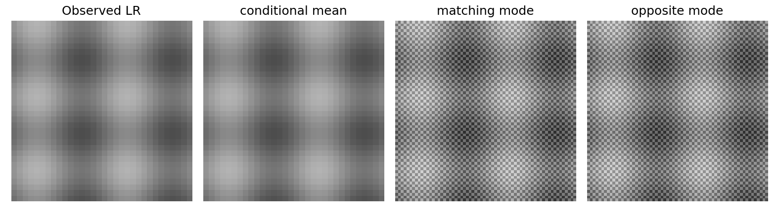
Consider ×2 block averaging, , which replaces each 2 × 2 block by its mean. A checkerboard with values sums to zero inside that block. Adding or subtracting it changes HR texture without changing the observed LR image. The texture lies in the null space of .
The following synthetic experiment builds a smooth LR pattern and two opposite HR textures. It compares a conditional mean with two plausible modes. We deliberately know the measurement model here; real-world photos make consistency checking harder because that model must itself be estimated.
Code · Python · 15 lines
import numpy as np

row, col = np.mgrid[:32, :32]
lr = 0.5 + 0.12*np.sin(2*np.pi*col/16) + 0.08*np.cos(2*np.pi*row/13)
base = lr.repeat(2, 0).repeat(2, 1)
i, j = np.indices(base.shape)
texture = 0.12*(-1.)**(i+j)  # zero mean in every 2x2 block
truth = base + texture
candidates = {'conditional mean': base, 'matching mode': base+texture, 'opposite mode': base-texture}
def measure(x):
    return x.reshape(32,2,32,2).mean((1,3))
for name, x in candidates.items():
    mse = np.mean((x-truth)**2)
    discrepancy = np.max(np.abs(measure(x)-lr))
    print(f'{name:16s} MSE {mse:.4f} | LR discrepancy {discrepancy:.1e}')
Output
conditional mean MSE 0.0144 | LR discrepancy 0.0e+00
matching mode    MSE 0.0000 | LR discrepancy 5.6e-17
opposite mode    MSE 0.0576 | LR discrepancy 5.6e-17
These are our calculated outputs. All candidates reproduce the LR observation up to floating-point rounding. The sharp opposite mode nevertheless has four times the conditional mean’s squared error against this chosen ground truth. If the two hidden texture signs are equally likely, the conditional mean minimizes expected squared error, while a randomly sampled plausible mode is not guaranteed to match the particular original. No amount of inference acceleration identifies a bit the observation never measured.
What is transferred from inference to training?
Multi-step restoration repeatedly calls a denoising network. A one-step model must learn a larger image-conditioned transformation, so adaptation, teacher sampling, discriminators or score regularizers can make training more demanding. Report both sides of the trade: fewer deployment calls may require substantial training machinery.
A pretrained text-to-image denoiser has not automatically learned that an LR image latent is a legitimate high-noise input. Feeding it such a latent without adaptation can fail. Methods such as OSEDiff explicitly train that image-to-image use [1]. The diffusion network is then a useful pretrained parameterization of a conditional restorer, rather than proof that the input follows its original forward-noise distribution.
A map of short-chain and one-step SR
Plain version. Some methods shorten a restoration-specific chain; some adapt a large pretrained prior; others learn the starting state or expose separate controls. Identify which component changes before comparing names.
| Family | Starting point | Main training signal | Representative method | What to check |
|---|---|---|---|---|
| Residual-shift chain | LR-centered noisy state | Image-conditioned diffusion reconstruction | ResShift [2] | Noise schedule, number of steps, training domain |
| Conditional endpoint distillation | LR plus an initial random perturbation | Teacher endpoints and a learned inverse/GT cycle | SinSR [3] | Teacher procedure and student’s actual one-step mapping |
| Pretrained-prior adaptation | LR image latent | Paired reconstruction plus latent score regularization | OSEDiff [1] | Encoder/decoder adaptation, prompt cost, auxiliary score tracking |
| Degradation-aware adaptation | LR latent with estimated degradation | Reconstruction, perceptual and adversarial losses | S3Diff [4] | Degradation estimator and guidance evaluation count |
| Adversarial distillation | Image-conditioned short sampler | Teacher and discriminator | AddSR [5] | Training version and inference budget |
| Target-aware score training | LR-conditioned student | Paired target scores and distribution-aware training states | TSD-SR [6] | How target HR information enters training |
| Learned inversion/start | Predicted image-conditioned noisy state | Loss after a pretrained reverse process | InvSR [7] | Starting-state predictor and total number of calls |
| Separate enhancement controls | LR latent | Pixel and semantic LoRA objectives | PiSA-SR [8] | Which weights are varied and whether fidelity changes monotonically |
The categories overlap. The table is a functional map, not an exclusive taxonomy. A pretrained one-step generator, a learned start and an adversarial objective can occur in the same system. Some methods support several inference budgets; a four-step score must retain its four-step label.
The larger field is organized in the blind-SR and diffusion-SR surveys [9], [10]. Their degradation assumptions remain important here. Fast inference does not make a model trained on one synthetic degradation distribution robust to every camera, codec or historical photograph.
A short chain centered on the observation
Plain version. Shift the high-resolution image toward the low-resolution observation rather than pure noise, so reversal starts near observed structure.
ResShift defines a residual between the enlarged LR image and HR target [2]. A convenient expression for its forward marginal is
Here increases from near zero toward one, scales noise, and is the identity covariance. Image dimensions match because has been enlarged, or both images have been encoded into matching latent grids. Near the final forward time, the state is approximately LR-centered Gaussian noise; reversing the chain restores detail.
The network predicts the HR target from a noisy state, the observation and time. Training therefore learns a restoration-conditioned process. The published latent implementation uses an image autoencoder and a short default chain. This is different from freezing a large text-to-image prior and adding a controller. Its capacity, training images and representation differ, so score differences with a large pretrained prior do not isolate the chain length alone.
SinSR constructs a deterministic version of the ResShift reverse process, then distills its endpoint into one student prediction [3]. It also trains an inverse mapping and uses ground-truth reconstructions through that inverse. The student is not merely ResShift evaluated once with an unchanged prediction target.
A deterministic teacher mapping fixes the output associated with each LR-centered random start. It makes endpoint regression well defined, while the random start can still select different results. The ground-truth consistency term gives the student a paired-data signal beyond reproducing the teacher’s endpoint. Its use of the same network in inverse and restoration directions is a training design; inference only needs the restoration direction.
Optional: ResShift and SinSR (in the Paper guides). The forward model, deterministic coefficients, three training losses and the corresponding experiments.
Starting from an LR latent: OSEDiff
Plain version. OSEDiff converts an input-derived representation to a high-resolution latent in one network call; a separate training regularizer encourages natural outputs.
The deployed path
The model has an adapted image encoder , an adapted diffusion denoiser , a frozen image decoder , and a prompt extractor [1]. With input enlarged to the working resolution, write
Here is the LR-derived latent, text conditioning, the selected fixed diffusion timestep, and signal/noise coefficients in the paper’s notation. The formula does not add fresh Gaussian noise to . It is a learned image-to-image transformation at a fixed model timestep. The denoiser output is adapted for this use; the degraded latent is not assumed to be a genuine sample of the original high-noise forward process.
LoRA adds low-rank trainable updates to the pretrained encoder and denoiser [11]. Freezing the decoder keeps the representation’s output interpretation tied to the pretrained latent space. A small trainable parameter count describes adaptation size, not the total parameters or memory required to execute the pretrained network.
Paired fidelity and a learned prior
OSEDiff combines pixel MSE and LPIPS reconstruction with variational score distillation (VSD) [12], [13]. The first two terms compare outputs with paired HR training targets. The score regularizer compares the distribution of generated latents with a pretrained natural-image prior, using a fixed pretrained denoiser and a second denoiser adapted to current generated samples.
This is the restoration counterpart of the distribution-matching idea in DLCV 12B. It does not directly calculate the unknown real-world degradation likelihood. The paired synthetic examples teach how to preserve content under sampled damage; the prior regularizer teaches natural appearance. Both may be wrong for a particular out-of-distribution input.
Why regularize in latent space?
A pixel-space prior-gradient calculation can repeatedly decode a generated latent and encode the resulting image again. OSEDiff approximates that round trip by operating directly on the predicted latent. This reduces repeated encoding/decoding on the regularization path. It relies on the pretrained autoencoder’s representation being sufficiently consistent; it is an approximation, not an exact identity for arbitrary latents.
The auxiliary regularizer networks are training-time components. Deployment still includes image encoding, prompt extraction, one denoiser pass and image decoding. A paper’s timing must state which of these were measured. A change from a lightweight tag extractor to a large captioning model can erase much of the practical speed benefit even when the denoiser still runs once.
Optional: OSEDiff (in the Paper guides). Every component, the latent-space gradient, training data, score tables, encoder/decoder studies, prompt costs and LoRA-rank ablations.
Making adaptation depend on the damage
Plain version. One fixed correction is not equally suitable for slight blur and heavy noise. S3Diff changes the low-rank adaptation according to an estimated degradation description [4].
For a weight matrix , ordinary LoRA gives , with and for a small rank . S3Diff introduces a degradation-conditioned middle matrix:
Here identifies a network block, contains estimated blur/noise information, and modulates the low-rank update. A shared mapping uses degradation embeddings and block identifiers to produce block-specific corrections. Different images can therefore receive different effective updates.
The degradation vector is an estimate, not complete knowledge of the camera pipeline. If it is wrong or fails to describe compression and spatial variation, the adaptive correction can be wrong too. The method is also different from a single static LoRA that can be merged once for all inputs: an input-dependent correction still requires input-dependent computation.
S3Diff uses generic positive/negative quality prompts and online negative targets rather than requiring a semantic captioner for every image. The training mixture teaches the meaning of poor-quality output. Classifier-free guidance can then combine differently conditioned predictions. If that configuration makes two denoiser predictions, count both when reporting NFE even though there is only one state-update step.
Optional: S3Diff (in the Paper guides). Dynamic matrices, block embeddings, online negative prompting and measured adaptation trade-offs.
Other ways to improve a short restoration map
Plain version. Once the chain is short, errors in conditions, targets and starting states matter more. Recent methods address different parts of that problem instead of only reducing the step count further.
Adversarial restoration distillation
AddSR applies adversarial diffusion distillation to image-conditioned restoration [5], [14]. A pretrained teacher supplies restoration knowledge, while a discriminator pushes outputs toward realistic images. The method combines conditioning and distillation rather than simply applying a text-to-image one-step generator to the enlarged input.
An adversarial objective can add convincing detail without proving that the detail is correct. Check the teacher, restoration conditioning, number of inference steps and training version. A method that supports a few steps should not have its best few-step result relabeled as one-step performance.
Target-aware scores and training states
TSD-SR observes that a pretrained teacher can provide unreliable directions on poor student outputs, especially early in training [6]. It introduces a target-score construction that uses the paired HR training latent, and a distribution-aware sampling module that produces training states closer to the adapted diffusion trajectory.
The paired target is available during training, not at deployment. Comparing the teacher’s predictions on a generated latent and its paired target supplies an additional direction beyond comparing teacher and current-student scores. This is a change to the regularization target, not direct evidence that all teacher-score errors have been eliminated. The sampling module also costs training work, even if it is discarded from a one-step inference pipeline.
Learning where the reverse process starts
InvSR learns an image-conditioned noise/start predictor and runs a pretrained reverse process from the predicted state [7]. At the starting point, the predicted “noise” need not be independent standard Gaussian noise; it can be correlated with the observed image to compensate for replacing an unknown clean image with its LR observation.
This is not the same as taking an arbitrary off-the-shelf inversion of a real photograph. The starting-state model is trained for restoration, with losses evaluated after the chosen reverse process. It can support different selected step budgets, but a learned starting-state predictor adds a network call. One reverse denoising step therefore need not equal one total model evaluation.
Separating pixel and semantic enhancement
PiSA-SR trains two low-rank update groups: one for pixel reconstruction and another for semantic/perceptual enhancement [8]. The first is trained before the second; the semantic stage holds the learned pixel update fixed. The default inference uses one combined prediction. Its adjustable configuration computes pixel- and semantic-enhanced outputs separately and uses two diffusion evaluations; separate weights then alter the residual contributions.
That adjustable setting must be counted separately from the default one-step setting. These controls change a learned model’s behavior. They do not physically separate every pixel into a “factual” and “invented” channel, and metric responses need not be monotonic. PiSA-SR uses a classifier-score-distillation objective rather than maintaining the same generated-distribution score model as OSEDiff. The change reduces some training machinery while changing the statistical objective; it is not an algebraically identical shortcut to the same VSD loss.
Optional: TSD-SR, InvSR and PiSA-SR (in the Paper guides). The components and evidence behind these different interventions.
Fidelity, realism and control
Plain version. Making an output agree with a natural-image prior does not necessarily make it agree with the observation. A fidelity term and a realism term can pull in different directions.
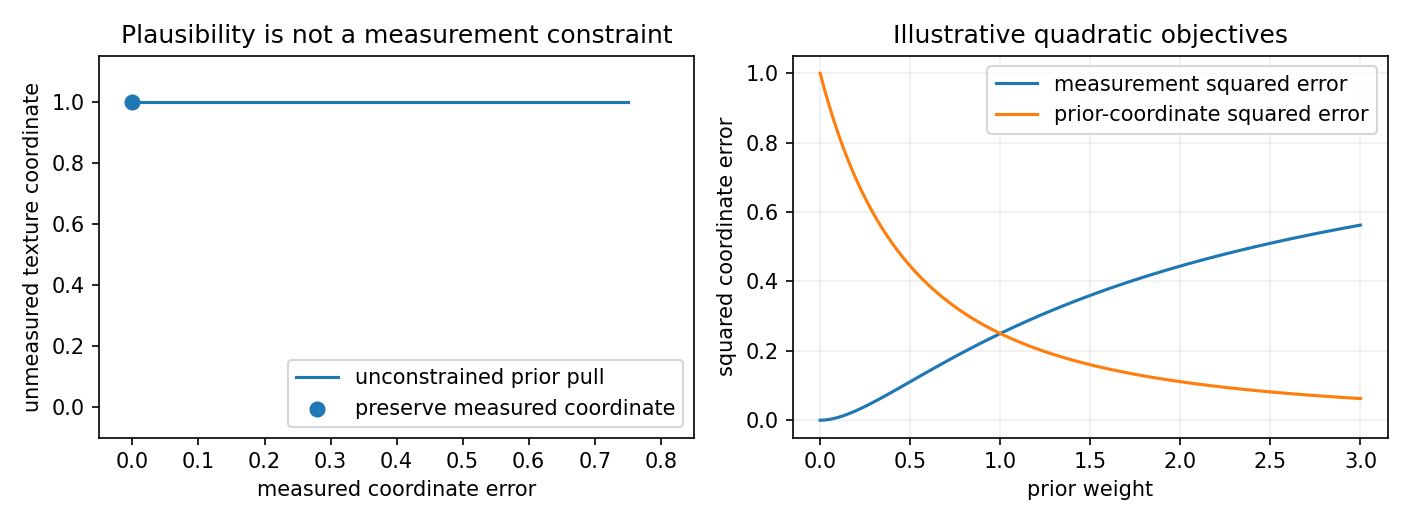
For an illustrative quadratic problem, let represent an error in a measured coordinate and an unmeasured texture coordinate. Suppose a prior prefers while the observation constrains . Minimizing gives and when . Stronger prior weight changes a coordinate the observation actually constrains. A separate constraint would protect that coordinate, but would still leave the texture’s correctness unresolved.
Here is a hypothetical objective weight, not a measured hyperparameter of any cited model. The example explains why “more realistic” is not synonymous with “more faithful.” In a neural restorer the coordinates are not cleanly separated, the degradation is unknown, and pixel/perceptual losses are trained over a dataset rather than solved exactly for each input.
Useful controls include a prior-loss weight during training, a feature/residual strength at inference, a guidance scale, a degradation estimate or a selected starting noise level. They are not interchangeable. A training-loss weight usually requires retraining; an inference coefficient changes one fitted model; choosing another checkpoint may change both training data and objectives. State which operation produces a comparison.
For text, faces and repeated structure, inspect whether the model changes discrete content: a letter, identity cue, brick count or boundary. Repeatability helps compare settings but does not establish factual correctness. For evidence-sensitive use, retain the original and describe generated detail as a hypothesis rather than treating a sharper output as an additional measurement.
Measuring speed and quality honestly
Plain version. Count everything a user waits for, and keep the quality protocol attached to the timing row. A smaller adaptation file or one diffusion update is not a complete speed measurement.
The pipeline to time
A typical system performs resizing, image encoding, optional degradation estimation, optional prompt extraction, generation/denoising, decoding and postprocessing. Some systems also use tiling. Record input resolution and output resolution, device, precision, batch size, warm-up, synchronization and whether text features are cached.
For OSEDiff, its Table 2 reports 0.11 seconds on an A100 under a stated 512 × 512 input-size test; the prompt-extractor study separately reports costs [1]. Do not assume the same timing boundary as another paper’s 128-to-512 benchmark. A rigorous reproduction should inspect the timing code and report prompt extraction separately if its inclusion is unclear. At high resolutions, tiled encoding and decoding can become substantial even when there is only one denoiser call.
Distinguish trainable parameters, total model parameters, peak inference memory and adaptation-file size. LoRA can reduce the first and last without proportionally reducing the frozen backbone required for inference. Dynamic LoRA, prompt extraction and learned inversion add their own work. Even static adapters merged into a backbone do not make its matrix multiplications disappear.
The quality protocol
Use full-reference fidelity and perceptual metrics on synthetic or captured pairs, and no-reference measurements plus inspection on unpaired real images [15], [16], [17]. PSNR and SSIM measure different aspects of reference agreement; LPIPS and DISTS compare perceptual representations [18], [12], [19]. NIQE, MUSIQ, MANIQA and CLIPIQA predict aspects of visual quality without an HR reference [20], [21], [22], [23]. They do not verify the original scene.
Keep channel, border crop, resizing, alignment and random seed conventions fixed. A method can improve a no-reference score by adding texture and worsen reference fidelity. On captured pairs, slight misregistration affects pixel metrics. On synthetic tests, matching a model’s own training degradation may favor it. The detailed evaluation caveats remain those in DLCV 09A.1.
For stochastic models, report variability across seeds rather than choosing only an attractive output. For deterministic models, examine multiple image types and damages rather than interpreting a single repeatable output as robustness. Evaluate letters, small faces, flat regions and regular grids separately, because an average score can hide different failure mechanisms.
Modern view
Plain version. Shortening inference has exposed several distinct learning problems: choose a useful start, preserve observed content, estimate a reliable prior direction and offer understandable controls.
Liu et al.’s blind-SR survey [9] distinguishes explicit degradation modeling, implicit data-distribution learning and single-image information. It helps identify what uncertainty an efficient model still assumes away. Moser et al.’s diffusion-SR survey [10] organizes diffusion restoration by domain, conditioning and generative process; it places short-chain designs within a larger set of fidelity and computation trade-offs. Fan et al.’s distillation survey [24] supplies a complementary objective-based view: endpoint fidelity, trajectories and adversarial learning are different supervision sources.
The 2023–2025 sequence is not a single replacement chain. ResShift changes the restoration process; SinSR distills its conditional endpoint; OSEDiff adapts a large pretrained prior with score regularization; S3Diff adapts to degradation; TSD-SR changes score targets and training states; InvSR learns the start; PiSA-SR separates enhancement controls [2], [3], [1], [4], [6], [7], [8]. Each addresses a different bottleneck, and their benchmark distributions and backbones differ.
The 2026 TUDSR work uses a twice-upsampling/diffusion design for higher-scale restoration [25]. It is relevant to how short diffusion components scale into a complete upsampling system, but multiple stages should be counted as multiple stages rather than advertised as one total operation. New architecture or scale settings also require renewed fidelity and cost comparisons.
Open problems include uncertain degradation, reliable text and identity preservation, score estimates on poor generated samples, generalization beyond synthetic processing, large-image tiling, and controls that users can understand without learning training terminology. A practical interface should expose meaningful visual choices and preserve the input for comparison. It should not imply that an “enhance detail” setting recovers information that was never measured.
Key takeaways
- An observation-derived start saves work only when trained for the intended image-to-image use.
- One-step inference describes a budget; methods can use different training objectives.
- ResShift/SinSR compress a restoration process; OSEDiff adapts a pretrained prior.
- Latent encoding, prompts, decoder choices and auxiliary training each have separate roles and costs.
- Determinism and low-resolution consistency do not establish correct missing detail.
- Measure the whole pipeline and compare fidelity, preference, semantic correctness and variability.
Exercises
- Null-space ambiguity. Change the checkerboard amplitude in the experiment. Derive the squared errors of the conditional mean and opposite texture, and check that the LR measurements remain unchanged.
Hint
For amplitude , each texture value has magnitude , so the mean’s MSE is and the opposite mode’s MSE is . Each 2 × 2 texture sums to zero. Keep the amplitude small enough that clipping does not alter the measurement equation.
- A wrong consistency test. Replace block averaging with a mildly blurred resize while keeping the same HR candidates. Do identical old block averages guarantee identical new LR images? Explain what this says about testing real-world consistency with an estimated degradation.
Hint
Null spaces depend on the operator. A texture annihilated by one downsampler need not be annihilated by another. Agreement under a guessed operator is evidence conditional on that operator, not proof about the unknown camera pipeline.
- Training-time and inference-time networks. Draw the OSEDiff computation and mark the encoder, denoiser, decoder, prompt extractor, fixed regularizer and adapted regularizer. Which networks receive generator gradients, and which execute at deployment?
Hint
The generator’s adapted encoder and denoiser are updated by reconstruction and prior signals. The decoder is fixed. The adapted regularizer has its own denoising objective. The two regularizers are discarded at deployment; the prompt extractor remains unless prompts are supplied or a different configuration is used.
- Count dynamic guidance. A method predicts one updated state but evaluates positive and negative prompts separately, and also calls a degradation estimator and VAE encoder/decoder. What can be called one step, and what should a timing report count?
Hint
There is one state-update step but two prompt-conditioned denoiser evaluations. Include degradation estimation, encoding and decoding in end-to-end timing; report any batching convention. A cached prompt embedding reduces text-encoder work, not the two denoising predictions themselves.
- A meaningful control. Design a comparison for a “more detail” control using flat sky, small text and repeated windows. State one fidelity check, one visual-quality check and one failure that an average no-reference score could miss.
Hint
Compare the same inputs and crops across settings. Check changed letters and window boundaries, inspect new sky texture, and record a quality metric without treating it as truth. A setting can improve an aggregate score while changing a discrete character or repeating a false pattern.
References
- R. Wu, L. Sun, Z. Ma, L. Zhang, “One-Step Effective Diffusion Network for Real-World Image Super-Resolution,” NeurIPS, 2024. source
- Z. Yue, J. Wang, C. C. Loy, “ResShift: Efficient Diffusion Model for Image Super-resolution by Residual Shifting,” NeurIPS, 2023. source
- Y. Wang, W. Yang, X. Chen, et al., “SinSR: Diffusion-Based Image Super-Resolution in a Single Step,” CVPR, 2024. source · supplementary ablations
- A. Zhang, Z. Yue, R. Pei, W. Ren, X. Cao, “Degradation-Guided One-Step Image Super-Resolution with Diffusion Priors,” arXiv preprint, 2024. paper
- Y. Tai, R. Xie, C. Zhao, K. Zhang, Z. Zhang, J. Zhou, J. Yang, “AddSR: Accelerating diffusion-based blind super-resolution with adversarial diffusion distillation,” Pattern Recognition, 2026. published version · manuscript supplying the discussed tables
- L. Dong, Q. Fan, Y. Guo, Z. Wang, Q. Zhang, J. Chen, Y. Luo, C. Zou, “TSD-SR: One-Step Diffusion with Target Score Distillation for Real-World Image Super-Resolution,” CVPR, 2025. paper
- Z. Yue, K. Liao, C. C. Loy, “Arbitrary-steps Image Super-resolution via Diffusion Inversion,” CVPR, 2025. paper
- L. Sun, R. Wu, Z. Ma, S. Liu, Q. Yi, L. Zhang, “Pixel-level and Semantic-level Adjustable Super-resolution: A Dual-LoRA Approach,” CVPR, 2025. paper
- A. Liu, Y. Liu, J. Gu, Y. Qiao, C. Dong, “Blind Image Super-Resolution: A Survey and Beyond,” IEEE TPAMI (early access), 2022. source
- B. B. Moser, A. S. Shanbhag, F. Raue, S. Frolov, S. Palacio and A. Dengel, “Diffusion Models, Image Super-Resolution, and Everything: A Survey,” IEEE Transactions on Neural Networks and Learning Systems, vol. 36, no. 7, pp. 11793–11813, 2025. doi · arXiv
- E. J. Hu, Y. Shen, P. Wallis, Z. Allen-Zhu, Y. Li, S. Wang, L. Wang, W. Chen, “LoRA: Low-Rank Adaptation of Large Language Models,” ICLR, 2022. source
- R. Zhang, P. Isola, A. A. Efros, E. Shechtman and O. Wang, “The Unreasonable Effectiveness of Deep Features as a Perceptual Metric,” in Proc. IEEE/CVF CVPR, 2018, pp. 586–595. doi · arXiv
- Z. Wang, C. Lu, Y. Wang, F. Bao, C. Li, H. Su, J. Zhu, “ProlificDreamer: High-Fidelity and Diverse Text-to-3D Generation with Variational Score Distillation,” NeurIPS, 2023. paper
- A. Sauer, D. Lorenz, A. Blattmann, R. Rombach, “Adversarial Diffusion Distillation,” ECCV, 2024. paper
- J. Cai, H. Zeng, H. Yong, Z. Cao, L. Zhang, “Toward Real-World Single Image Super-Resolution: A New Benchmark and a New Model,” Proceedings of the IEEE/CVF International Conference on Computer Vision, 2019. source
- P. Wei, Z. Xie, H. Lu, Z. Zhan, Q. Ye, W. Zuo, L. Lin, “Component Divide-and-Conquer for Real-World Image Super-Resolution,” ECCV, 2020. source
- E. Agustsson and R. Timofte, “NTIRE 2017 Challenge on Single Image Super-Resolution: Dataset and Study,” in Proc. IEEE CVPR Workshops, 2017, pp. 1122–1131. doi · CVF
- Z. Wang, A. C. Bovik, H. R. Sheikh and E. P. Simoncelli, “Image Quality Assessment: From Error Visibility to Structural Similarity,” IEEE Transactions on Image Processing, vol. 13, no. 4, pp. 600–612, 2004. doi
- K. Ding, K. Ma, S. Wang, E. P. Simoncelli, “Image Quality Assessment: Unifying Structure and Texture Similarity,” IEEE TPAMI, 2022. source
- A. Mittal, R. Soundararajan and A. C. Bovik, “Making a “Completely Blind” Image Quality Analyzer,” IEEE Signal Processing Letters, vol. 20, no. 3, pp. 209–212, 2013. doi
- J. Ke, Q. Wang, Y. Wang, P. Milanfar, F. Yang, “MUSIQ: Multi-scale Image Quality Transformer,” ICCV, 2021. source
- S. Yang, T. Wu, S. Shi, S. Lao, Y. Gong, M. Cao, J. Wang, Y. Yang, “MANIQA: Multi-dimension Attention Network for No-Reference Image Quality Assessment,” CVPR Workshops, 2022. source
- J. Wang, K. C. K. Chan, C. C. Loy, “Exploring CLIP for Assessing the Look and Feel of Images,” AAAI, 2023. source
- X. Fan, Z. Wu, H. Wu, L. Cao, “A Survey on Pre-Trained Diffusion Model Distillations,” arXiv preprint, version 2, 2025. paper
- Z. Wu, Y. Dong, X. Wei, “TUDSR: Twice Upsampling-Diffusion for Higher Super-Resolution,” CVPR, 2026. paper
- P. Esser, R. Rombach, B. Ommer, “Taming Transformers for High-Resolution Image Synthesis,” CVPR, 2021. paper
- X. Wang, L. Xie, C. Dong, Y. Shan, “Real-ESRGAN: Training Real-World Blind Super-Resolution With Pure Synthetic Data,” Proceedings of the IEEE/CVF International Conference on Computer Vision, 2021. source
- J. Deng, W. Dong, R. Socher, L. Li, Kai Li, Li Fei-Fei, “ImageNet: A large-scale hierarchical image database,” CVPR, 2009. doi
- R. Rombach, A. Blattmann, D. Lorenz, P. Esser, B. Ommer, “High-Resolution Image Synthesis with Latent Diffusion Models,” CVPR, 2022. source
- R. Wu, T. Yang, L. Sun, Z. Zhang, S. Li, L. Zhang, “SeeSR: Towards Semantics-Aware Real-World Image Super-Resolution,” Proceedings of the IEEE/CVF Conference on Computer Vision and Pattern Recognition, 2024. source · supplementary experiments
- H. Liu, C. Li, Q. Wu, Y. J. Lee, “Visual Instruction Tuning,” NeurIPS, 2023. source
- Y. Li, K. Zhang, J. Liang, et al., “LSDIR: A Large Scale Dataset for Image Restoration,” CVPR Workshops, 2023. paper
- T. Karras, S. Laine, T. Aila, “A Style-Based Generator Architecture for Generative Adversarial Networks,” CVPR, 2019. paper
- I. Loshchilov, F. Hutter, “Decoupled Weight Decay Regularization,” ICLR, 2019. paper
- P. Esser, S. Kulal, A. Blattmann, et al., “Scaling Rectified Flow Transformers for High-Resolution Image Synthesis,” ICML, 2024. paper
- J. Ho, T. Salimans, “Classifier-Free Diffusion Guidance,” arXiv preprint, 2022. paper
- R. Timofte, E. Agustsson, L. Van Gool, M.-H. Yang, L. Zhang et al., “NTIRE 2017 Challenge on Single Image Super-Resolution: Methods and Results,” in Proc. IEEE CVPR Workshops, 2017, pp. 1110–1121. doi · CVF
Check your understanding
This tutorial has 5 exercises. Can you solve them without opening the hints?
Go to the exercises ↑Next DLCV 09A.3 · Video Super-Resolution: Using Time to Recover Detail · 36 min