DLCV 12B · One-Step Generation
Needs: ML 08 · Diffusion Models and Flow Matching, DLCV 12 · Image Generation: From GANs to Text-to-Image Systems
Navigate: this page and this track: Navigate: this page and this track
On this page
- What you’ll learn1 min
- The big picture1 min
- Why taking one large step is different3 min
- A map of acceleration methods2 min
- Compressing teacher trajectories2 min
- Endpoint agreement with consistency models2 min
- Straightening before distilling1 min
- Adding a realism signal1 min
- Matching distributions rather than individual endpoints2 min
- Learning finite jumps directly2 min
- Evaluating the complete trade-off2 min
- Failure modes and choosing a family1 min
- Modern view1 min
- Key takeaways1 min
- Exercises2 min
- Supplementary notes
- Paper guides
- References
- Progressive Distillation: two teacher moves in one student move (ICLR 2022)
- Consistency Models: the same endpoint along a path (ICML 2023)
- InstaFlow: reflow, then endpoint distillation (ICLR 2024)
- Latent Consistency Models: endpoints in a guided latent flow (2023)
- Adversarial Diffusion Distillation: a teacher and a discriminator (ECCV 2024)
- DMD: matching a teacher-defined distribution (CVPR 2024)
- DMD2: tracking the student and using real data (NeurIPS 2024)
Deep Learning for Computer Vision
What you’ll learn
- Explain why one local denoising direction may not reach a distant endpoint.
- Compare endpoint regression, consistency, reflow and distribution matching.
- Distinguish matching teacher trajectories from matching output distributions.
- Understand step-size-conditioned shortcuts and average-velocity targets.
- Report network evaluations, complete latency, alignment and diversity.
The big picture
A diffusion denoiser usually predicts a local correction at a particular noise level. A one-step generator must turn a random input into a complete sample. It therefore needs a finite change, not merely a more confident local correction. This chapter covers diffusion distillation, consistency models, rectified flows and shortcut/average-velocity models together. Some borrow a pretrained teacher; others train a generator directly. “One-step” describes inference, not a single common training algorithm.
Read ML 08: Diffusion Models and Flow Matching first for noising schedules, prediction targets and probability-flow equations. DLCV 12: Image Generation supplies the image-generation pipeline and its evaluation context. Here the main question is narrower: what must change when the iterative part is compressed into one or a few calls? Super-resolution applies these ideas to an observed image rather than unconditional noise; that application has a separate one-step SR chapter.
For a first pass, read the numerical example, the family table and the evaluation checklist. Then choose a detailed paper introduction. The equations distinguish training objectives; understanding every derivation is not required to understand the differences between the families.
Why taking one large step is different
Plain version. A local tangent gives the current direction, not the displacement to a distant endpoint. Accurate local predictions can still yield a poor one-step jump.
Write a probability-flow or flow-matching ordinary differential equation as
Here is the current image or latent vector, is continuous time, the instantaneous velocity, and a signed time increment. The approximation on the right is an Euler step. For a smooth field, its local error depends on how changes with time and position along the path. Making large discards those changes. A more accurate neural estimate of the same instantaneous field does not automatically repair this integration error.
There are three separate error sources: model error, because a learned field differs from its target; numerical error, because a finite-step solver approximates the learned continuous dynamics; and distribution mismatch, because the terminal noise, conditioning or resolution at inference differs from training. Improving one does not eliminate the others. Probability-flow theory [1] describes an ideal connection between marginal distributions; it is not a certificate that any finite neural sampler exactly follows it.
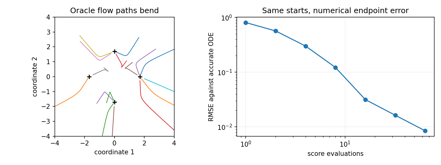
The same caution applies to flow matching [2]. Even when training pairs are interpolated along straight lines, the marginal velocity at a location averages directions from several possible pairs. Its resulting trajectories can bend. The straightness of the sampled training interpolation is therefore not the same as straightness of the learned marginal flow.
A toy where the score is known exactly
The following experiment removes neural-network error. Its target is an equally weighted mixture of four 2-D Gaussians. After adding Gaussian noise of standard deviation , each component variance is , where is the component standard deviation. The exact score is
Here is component ’s center and is its normalized posterior mixture weight at . For this additive-noise family, the probability-flow equation parameterized by noise scale is [3]. We integrate from large to small .
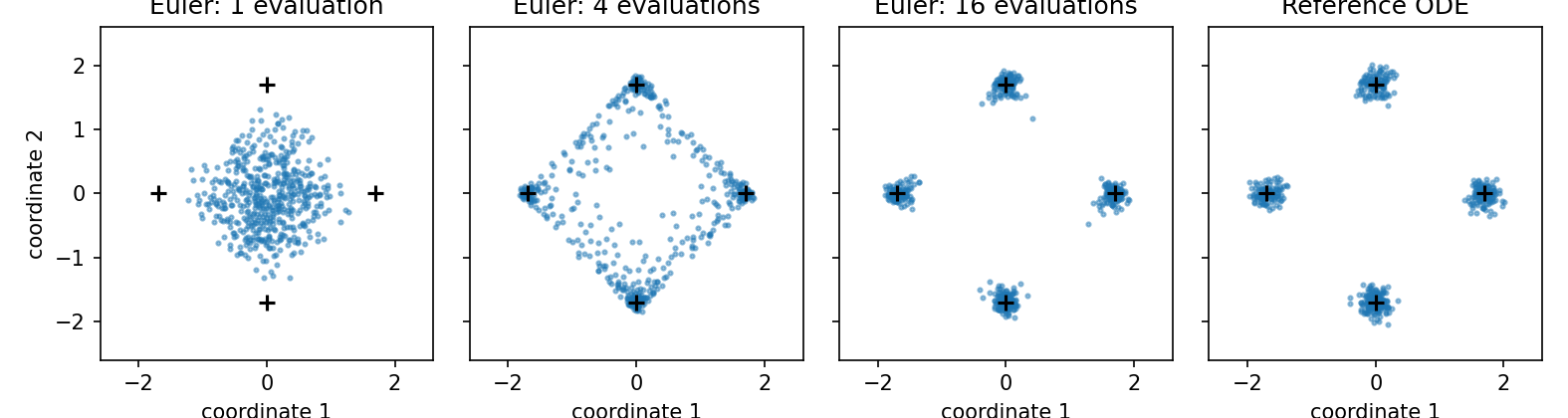
The initial samples are drawn from the exact noisy mixture, not assumed to be standard Gaussian. This makes the numerical comparison controlled. A real generator must also handle how well its chosen starting distribution matches the training boundary. We compare coarse Euler endpoints with an accurate adaptive ODE solution from the same initial points; the error is not an image-quality metric or a trained-model benchmark.
Code · Python · 33 lines
import numpy as np
from scipy.integrate import solve_ivp

centers = np.array([[-1.7, 0.], [1.7, 0.], [0., -1.7], [0., 1.7]])
base_var = 0.12**2
sigma_start, sigma_end = 3.0, 0.04

def score(x, sigma):
    """Exact score of the equally weighted Gaussian mixture after Gaussian noising."""
    var = base_var + sigma**2
    delta = x[:, None, :] - centers[None, :, :]
    logits = -(delta**2).sum(-1) / (2 * var)
    weights = np.exp(logits - logits.max(1, keepdims=True))
    weights /= weights.sum(1, keepdims=True)
    return -(weights[:, :, None] * delta).sum(1) / var

def euler(initial, steps):
    x = initial.copy()
    grid = np.linspace(sigma_start, sigma_end, steps + 1)
    for s0, s1 in zip(grid[:-1], grid[1:]):
        x += (s1 - s0) * (-s0 * score(x, s0))
    return x

rng = np.random.default_rng(7)
initial = centers[rng.integers(4, size=512)] + np.sqrt(base_var + sigma_start**2) * rng.normal(size=(512, 2))
shape = initial.shape
solution = solve_ivp(lambda sigma, flat: (-sigma * score(flat.reshape(shape), sigma)).ravel(),
                     (sigma_start, sigma_end), initial.ravel(), rtol=1e-9, atol=1e-10, dense_output=True)
reference = solution.y[:, -1].reshape(shape)
for steps in [1, 2, 4, 8, 16, 32, 64]:
    estimate = euler(initial, steps)
    rmse = np.sqrt(np.mean((estimate - reference)**2))
    print(f'{steps:2d} evaluations: endpoint RMSE {rmse:.4f}')
Output
 1 evaluations: endpoint RMSE 0.8098
 2 evaluations: endpoint RMSE 0.5686
 4 evaluations: endpoint RMSE 0.3011
 8 evaluations: endpoint RMSE 0.1224
16 evaluations: endpoint RMSE 0.0316
32 evaluations: endpoint RMSE 0.0164
64 evaluations: endpoint RMSE 0.0085
These are our seeded numerical results. One Euler evaluation has a large endpoint error despite using the exact score. More evaluations follow the curved flow more accurately. The adaptive reference is itself a numerical solution, with tight tolerances; it is not an analytic closed-form transport map.
A map of acceleration methods
Plain version. Separate faster integration of an existing model from training a new endpoint, jump or distribution predictor.
| Family | What is learned or changed | Needs a separate teacher? | Main constraint |
|---|---|---|---|
| Faster solver | A better numerical update for an existing field | Uses the existing field | Few-step accuracy still depends on the field and schedule |
| Progressive/trajectory distillation | Several teacher moves compressed into one student move | Yes | Student follows the selected teacher mapping |
| Consistency models | The same clean endpoint from different locations on one path | Distillation: yes; direct training: no | Accurate endpoint agreement across noise levels |
| Reflow and endpoint distillation | A more regular noise–image coupling, then a direct map | Usually a pretrained model for large image applications | Straightening and map approximation are separate stages |
| Adversarial distillation | Realistic outputs plus teacher-derived guidance | Yes in ADD/LADD | Discriminator stability and diversity |
| Distribution matching | Student output distribution agrees with a teacher-defined target | Yes | An auxiliary student score must track a changing distribution |
| Shortcut / average-velocity learning | Finite-interval moves conditioned on their interval | Can train from scratch | Self-target accuracy, time conditioning and boundary behavior |
The table follows the methodological separation in diffusion-distillation surveys [4], with direct-training families added because this chapter’s scope is one-step generation rather than distillation alone. Categories overlap. DMD2 combines distribution matching and an adversarial objective; InstaFlow combines reflow and endpoint distillation. A model’s training losses are more informative than assigning it one permanent label.
DDIM [5] and DPM-Solver [6] are useful baselines before training a student. They reduce discretization error per evaluation but do not, by themselves, learn a complete endpoint map. A comparison with an inefficient sampler can exaggerate a distilled model’s speed advantage. Conversely, a solver that works well at moderate step counts may still fail when forced into one evaluation.
Compressing teacher trajectories
Plain version. A teacher assigns a destination to each noisy input. Endpoint regression trains the student to reproduce that chosen mapping directly.
Progressive distillation
Progressive Distillation [7] repeatedly trains one student step to match two deterministic teacher steps. After training, the student becomes the teacher and the sampling budget is halved again. This gives a curriculum of larger jumps instead of asking a fresh network to approximate the whole map immediately.
Let a deterministic teacher take through an intermediate time to . A DDIM-style single update based on clean prediction is
Here are noisy states, and are the signal and noise schedule coefficients. Solving this affine equation for gives the student target that reproduces the teacher’s two-step endpoint. The target depends on the selected teacher mapping and starting state. It differs from ordinary clean-image denoising, whose squared-error optimum can average several compatible clean images.
This approach transfers work to training: many teacher evaluations produce targets while inference becomes cheaper. It can accumulate approximation error across stages. A student may need a particular schedule and output parameterization, so loading it into an arbitrary sampler is not equivalent to the trained procedure.
Optional: Progressive Distillation (in the Paper guides). The exact target, stable parameterizations, reported scores and stage-by-stage limitations.
Coupling is part of the target
There are many valid maps from a noise distribution to an image distribution. A trajectory teacher chooses one coupling: which output belongs to which random input. Matching that pair is stronger than matching only the output distribution.
A small example makes the distinction concrete. Consider a random input whose sign can select one of two target modes. The maps and have the same balanced output distribution when is symmetric. They have opposite samplewise correspondence. A pairwise regression loss strongly penalizes replacing one with the other even though neither changes the marginal distribution.
This is why one-step generation is not intrinsically “too deterministic.” A deterministic map of a random latent input can generate diverse outputs. Collapse occurs when the map ignores parts of that input or covers too few target modes. Averaging endpoints from unrelated random seeds during regression creates a different problem: the average can lie between modes and be an implausible sample.
Endpoint agreement with consistency models
Plain version. Instead of learning the next small correction, learn where a path ends. Two states on the same path should give the same answer.
A consistency function satisfies
for states on a shared probability-flow trajectory, with its near-clean endpoint at a small positive boundary time . A neural parameterization enforces the boundary condition through
where is a learned network, , and . Thus the boundary returns its input instead of allowing the same constant output everywhere. Boundary anchoring and proper training pairs matter: “make two predictions agree” alone has trivial solutions.
Consistency distillation uses a pretrained score model and a numerical solver to construct neighboring path states. The student output at the noisier state matches a stopped-gradient target-model output at the cleaner state. Consistency training learns from data without a separately pretrained diffusion teacher, using nearby noise levels and a shared-noise construction. They share the endpoint interpretation but differ in their supervision [8]. Later improvements change weighting, noise-level sampling and target-model updates [9]; the original configuration should not be treated as the final form of every consistency model.
One-step sampling evaluates at a noisy start. Few-step sampling alternates endpoint prediction with adding controlled noise at a lower level and predicting again. This can improve quality, but it is not simply repeating an identical deterministic map on its own output. A checkpoint trained for particular noise levels needs the corresponding sampling schedule.
Optional: Consistency Models (in the Paper guides). Boundary conditions, distillation versus direct training, and what the reported one- and two-step comparisons show.
Latent consistency and guidance
Latent Consistency Models (LCM) apply consistency distillation in a pretrained image autoencoder’s latent space [10], [11]. This reduces spatial computation but retains the cost and reconstruction limits of encoding/decoding. The denoiser becomes an endpoint predictor for the guided latent probability flow.
Classifier-free guidance normally combines conditional and unconditional network predictions. LCM conditions its student on guidance strength and distills the guided flow, so the chosen behavior can be produced without two separate denoiser predictions at each student step. The guidance range seen during training is part of the model’s usable interface. A guidance number in a distilled pipeline is not automatically interchangeable with the same number in the original pipeline: conventions and parameterizations differ.
LCM’s skipping-step construction pairs states farther apart during training than an immediately adjacent grid interval. This improves the usefulness of the consistency target for finite jumps. It still relies on the teacher and training schedule, and one-step outputs can be worse than two- or four-step outputs. “Supports one-step inference” is not a promise that one step is always the best operating point.
Optional: Latent Consistency Models (in the Paper guides). Guided endpoint parameterization, skipping intervals and the paper’s resolution-specific experiments.
Straightening before distilling
Plain version. A student learns a long move more easily if the teacher’s route is less tangled. Reflow changes the route before endpoint regression compresses it.
Rectified Flow [12] trains an instantaneous velocity using interpolated endpoint pairs. A reflow round samples a noise point , follows the current flow to , and trains another flow on the coupled pairs instead of independently pairing arbitrary noise and data. The resulting interpolation target is
Here time increases from noise at 0 to data at 1; is instantaneous velocity, and is the earlier model’s sampled endpoint map. This time direction differs from the noise-scale variable in the earlier toy. Writing the convention explicitly prevents a silent sign reversal.
Ideal reflow has useful distribution-preservation and transport-cost properties under its assumptions. A finite neural fit and approximate endpoint sampler introduce error. One reflow round does not guarantee globally straight learned trajectories. A network can still need several Euler evaluations after reflow; InstaFlow’s experiments distinguish this from subsequent one-step endpoint distillation [13].
The endpoint student can minimize , where is a text condition and a selected reconstruction/perceptual distance. This objective preserves the reflow teacher’s pairing. Reflow can change that pairing while preserving the ideal output marginal; endpoint regression then approximates the changed map. They solve related but different problems.
Optional: InstaFlow (in the Paper guides). Why direct distillation, one-step reflow and reflow followed by distillation have different results.
Adding a realism signal
Plain version. Matching a teacher endpoint can reproduce its errors. A discriminator supplies a second signal: does the student output look like the target data? This signal helps appearance but needs careful stabilization and evaluation of diversity.
Adversarial Diffusion Distillation (ADD) combines a pretrained student, a frozen diffusion teacher and a discriminator [14]. The student generates from selected noisy inputs. A diffusion-derived distillation term pulls its output toward a teacher denoising target, while an adversarial term rewards realistic appearance in pretrained feature space. The teacher and discriminator are training-time tools; neither must execute as an iterative teacher sampler during deployment.
For a generic adversarial formulation, a generator loss contains , where gives a realness score and the student output. The discriminator is trained to distinguish real and generated samples under its own loss and regularization. This scalar is a learned training signal, not a calibrated probability that an image is truthful or prompt-correct.
ADD supports refinement across a small set of trained noise levels. LADD moves adversarial distillation into latent diffusion feature representations, reducing the need to decode pixels and run a separate large image feature encoder during training [15]. The complete computational trade includes the teacher, discriminator and feature extraction during training, as well as the final decoder during inference.
Adversarial and diffusion losses do not guarantee diversity automatically. Inspect whether different random seeds yield different plausible compositions, whether uncommon prompt concepts survive, and whether apparent sharpness comes from repeated texture. A low FID can coexist with poor conditional coverage. Training stability, real-data access and how prompts condition the discriminator belong in any comparison.
Optional: ADD (in the Paper guides). The two training signals, initialization study and the difference between one-step and four-step preference results.
Matching distributions rather than individual endpoints
Plain version. A student can be rewarded for producing the right collection of images without being forced to copy the teacher’s exact image for every noise seed. That freedom can help, but the distribution of the student must be estimated while it keeps changing.
DMD learns a one-step generator and uses two diffusion score estimates [16]. One fixed model describes the teacher-defined target distribution. A second model learns the distribution of the student’s current outputs. At a common noise level, their score difference supplies a direction for moving generated samples toward the target.
Let and . A representative update has the form
Here is a random generator input, the condition, fresh Gaussian noise, the noising coefficients, a score, and a training weight. The equation is shorthand for the vector–Jacobian product back to generator parameters. Score estimates and time weighting make this a practical approximation; it is not an exact, directly evaluated image-density KL divergence.
Why include the student score? Following only a target score can push every sample toward already attractive modes, reducing diversity. The difference accounts for where the student already has probability mass. Why add noise? Clean generated and target distributions may have little overlapping support, while noising supplies a smoother comparison space. Why maintain a second diffusion network? The student output distribution changes after each generator update, so its score is not supplied by the fixed teacher.
Original DMD also uses a regression loss on teacher-generated noise–image pairs to stabilize learning and preserve coverage. This means the original method is not completely free of trajectory targets. SwiftBrush uses variational score-distillation ideas for text-to-image generation, while SiD derives score-identity-based objectives [17], [18]. These related methods should be compared through their actual objectives, weighting and data requirements rather than treated as identical implementations of one equation.
What DMD2 changes
DMD2 removes the offline endpoint-regression dataset and stabilizes the changing student-score estimate by updating it more often than the generator [19]. It also adds adversarial learning from real images to address errors in a teacher-defined target. The word “real” in a teacher-score diagram should therefore be read carefully: the fixed teacher’s score is an approximation, not direct access to the true data density.
For multi-step students, DMD2 trains on intermediate inputs produced by the student’s own sampling procedure. This reduces mismatch between teacher-noised training inputs and states the student actually visits. The method’s four-step large-model experiments are not evidence that an identically configured one-step large model has the same score. Steps, backbone, guidance and benchmark protocol must stay attached to every table row.
Optional: DMD and DMD2 (in the Paper guides). The score networks, regression trade-off, update-frequency ablation and multi-step input simulation.
Learning finite jumps directly
Plain version. A network can learn “move this far in time” rather than only “move in this direction now.” This changes its input and its target, so direct training can support large jumps without a separate teacher checkpoint.
Shortcut models
A shortcut model predicts a normalized displacement for a requested interval [20]. Its update is . At , training is grounded in a flow-matching velocity target. For longer intervals, one jump should agree with two consecutive shorter jumps:
Here is the current time, the shorter interval, and both terms use the same conditional generation task. The second term is evaluated at the updated position and time. A stopped-gradient target built from the shorter jumps trains the longer jump. Replacing the updated time by the original time would be a different objective.
Flow supervision prevents arbitrary self-consistency from being the only signal. The combined method can train in one phase, mixing local supervised targets with bootstrapped finite jumps. “No separate teacher” does not mean no self-targets, no training compute or no approximation error. Large jumps remain limited by network capacity and the accuracy of their bootstrapped targets.
Average velocity with MeanFlow
MeanFlow distinguishes an interval’s average velocity from its endpoint’s instantaneous velocity [21]. In a data-to-noise time convention, define
Here , is a point on the flow, instantaneous velocity and average velocity along the same trajectory. The integral is not approximated by calling once. A learned aims to represent its effect directly.
Differentiating the defining relation along the path gives
The derivative is total along the changing state, with held fixed. The training construction uses a Jacobian–vector product and a stopped-gradient target, so automatic differentiation can form the derivative without materializing a full image-sized Jacobian. The direct-training formulation replaces unavailable marginal velocity targets through its flow-matching construction. This identity is more informative than calling the method “Euler with bigger steps”: the learned quantity is different.
Both source time and destination time must be represented. At the average velocity approaches the instantaneous velocity. At the full noise-to-data interval, a single average-velocity evaluation supplies the intended whole displacement. Exact identities motivate the objective, while a finite trained network only approximates them. The paper’s JVP ablation demonstrates how sensitive this construction is to differentiating with respect to the correct variables.
Evaluating the complete trade-off
Plain version. A fast result is useful only if it still does the intended task. Evaluate the generated distribution, the conditioning, diversity and total cost together.
Steps, evaluations and time
A sampling step is a state update. A network function evaluation (NFE) is a network call. A solver can use multiple calls per update, and ordinary classifier-free guidance can require conditional and unconditional predictions. Batching those predictions may produce one API call but still process twice the examples. Report the convention explicitly; “one call” and “one example’s worth of denoiser compute” are not always the same.
Complete latency includes text encoding, condition extraction, denoising/generation, decoding and any postprocessing. Separate initialization and model loading from steady-state inference. Fix hardware, precision, resolution, batch size and synchronization; otherwise a claimed speedup can mix method improvements with system changes. Memory use also matters: a single large generator may exceed the deployment budget even though it runs only once.
If guidance has been baked into the student, count its absence as part of the trained system’s speed advantage, but also report the usable guidance range. If a prompt embedding is cached, say so. Comparing cached student text processing with uncached teacher processing does not measure only distillation.
Quality, alignment and diversity
FID compares means and covariances of image-feature distributions [22]. It does not compare corresponding image pairs and does not directly assess whether a requested relation is satisfied. The feature extractor, reference split, sample count and resizing affect the score. Small prompt subsets are not interchangeable with larger evaluation sets; FID-5k and FID-30k are different protocols.
CLIP-based similarity scores compare image and text embeddings [23]. Implementations differ in normalization, scaling and backbone. A score reported as 0.3 in one table and 30 in another may reflect scaling rather than a hundredfold quality difference. GenEval tests object, count, color and relational requirements using a structured evaluation protocol [24]. Such tests complement, rather than replace, human judgments and distribution metrics.
Diversity should be tested across prompts and across seeds for one prompt. A generator can cover many broad classes but repeatedly draw one composition for each condition. Conversely, a model can have high visual variation because it ignores the prompt. Evaluate the two together. Retaining a random input does not prove that the learned map uses it effectively.
Reading benchmark tables safely
A method may be tested on CIFAR-10, class-conditional ImageNet or text-conditioned COCO prompts [25], [26], [27]. Their scores answer different questions. A smaller-resolution unconditional result does not establish high-resolution prompt-following quality. Nor does a four-step result establish a one-step operating point.
For a useful comparison, record: the target task; backbone and initialization; training data and teacher; resolution; guidance convention; NFE; full latency and memory; distribution quality; conditional alignment; diversity; and uncertainty from finite samples. Use each paper’s own controlled ablations for claims about individual components. Cross-paper tables can show reported operating points, but cannot isolate causality when data, architecture and training budgets differ.
Failure modes and choosing a family
Plain version. Acceleration moves work and assumptions; it does not remove them. Choose the objective according to what must be preserved.
- Need the same endpoint for a given seed? Trajectory or endpoint regression is a natural starting point. It imposes a specific coupling and can copy teacher artifacts.
- Need a flexible step budget? Consistency, shortcut and interval-conditioned models explicitly support more than one budget, but require the trained sampling procedure.
- Need a new output distribution rather than exact teacher pairing? Distribution matching provides that freedom. Watch auxiliary-score lag, mode dropping and training stability.
- Need strong perceptual appearance? Adversarial terms can help, but evaluate diversity and conditioning rather than judging sharpness alone.
- Need no pretrained teacher? Direct consistency, shortcut or average-velocity training can fit that constraint. Compare complete training cost; removing a teacher checkpoint is not the same as making training inexpensive.
A one-step checkpoint can inherit the teacher’s biases, lose rare concepts, overfit an evaluation prompt set, or fail when controls are changed after distillation. Distribution objectives and self-targets have their own failure modes: inaccurate student scores, collapsed targets, poor boundary conditioning and train–test input mismatch. A model trained on a narrow time or guidance range should not be treated as a universal replacement for its teacher.
Modern view
Plain version. The field increasingly asks which object should be learned for a small inference budget, rather than assuming every improvement is a better approximation of the same denoising step.
Fan et al.’s distillation survey [4] organizes methods into fidelity/output objectives, trajectory methods and adversarial methods. Its taxonomy is useful for identifying what supervises a student and which parts of a teacher are retained. It does not imply that the categories are disjoint: DMD2 uses both distribution and adversarial signals. The broader diffusion survey by Yang et al. [28] places efficient sampling alongside model formulation and applications. Lipman et al.’s flow-matching guide [2] supplies a complementary transport view: local velocity, endpoint coupling and numerical integration are separate design choices.
From 2023 through 2025, consistency distillation, reflow, adversarial distillation and distribution matching produced different routes to few-step image generation. Shortcut models and MeanFlow show a separate direct-training route to finite jumps [20], [21]. Their class-conditional benchmark results should not be silently generalized to large text-to-image systems. The 2026 DMAD preprint explores adversarial distribution matching as an alternative to maintaining a separately updated student-score model [29]; its broader visual-generation setting and preprint status matter when comparing it with established image benchmarks.
Open problems include preserving rare modes and compositional control, maintaining editable conditioning after distillation, measuring quality beyond feature-distribution summaries, reducing training memory and compute, and transferring a one-step design across resolutions or domains. Speed alone is not a complete objective. For restoration, a further requirement appears: generated details should remain consistent with a particular observation. The one-step SR chapter applies this chapter’s ideas under that additional constraint.
Key takeaways
- A finite jump requires an endpoint or displacement target, not just a local direction used once.
- Separate solver error, learned-model error and train–test mismatch.
- Trajectory regression preserves a chosen coupling; distribution matching can learn a different one.
- Consistency needs boundary anchors; reflow changes coupling before compression into fewer steps.
- Distribution, adversarial and average-velocity objectives provide different supervision and estimation challenges.
- Compare full pipeline latency and network evaluations alongside quality, prompt adherence and diversity.
Exercises
- Oracle versus solver error. In the mixture example, compare a nonuniform noise-scale grid with the uniform grid at the same number of score evaluations. Where should more points be placed, and does that choice depend on the starting scale?
Hint
Inspect where the trajectories bend and where component assignments become sharp. Compare endpoint RMSE from the same initial samples. A better grid can improve a finite-step solver without changing its score. Avoid selecting the grid using a separate set of initial points and then calling its improvement universal.
- Endpoint or distribution? For symmetric Gaussian , compare and . Compute their expected squared pairwise difference and their output probabilities. Which objective can distinguish them?
Hint
Except on a probability-zero boundary, their values differ by 2, so the squared pairwise difference is 4. Both assign probability one half to each output. An ideal marginal-distribution comparison cannot distinguish them; a paired regression target can.
- A broken shortcut. In the two-short-jump equation, replace the second time by . Explain why this is not the same consistency relation, even if the network receives the updated state.
Hint
The vector field depends on time as well as position. For the scalar field , the two smaller Euler directions differ solely because time advances. A network asked for the original time on the second jump is answering the wrong interval query.
- Count the whole pipeline. A teacher uses 20 updates with two denoiser predictions per update. A student uses four updates with baked-in guidance. Both decode once, and each extracts a text embedding once. State the denoiser-evaluation ratio and explain why the wall-clock speedup need not equal it.
Hint
The denoiser evaluation counts are 40 and 4, a ratio of 10. Shared text encoding and decoding, batch efficiency, precision and memory behavior change the measured runtime ratio. Include those fixed costs in a simple timing model before predicting a deployment speedup.
- Diagnose a suspicious improvement. A student has lower FID but worse prompt-relation accuracy and nearly identical outputs across seeds. Propose three checks before accepting that it preserves its teacher’s generation quality.
Hint
Inspect per-prompt seed diversity, evaluate object and relation constraints on a held-out prompt set, and repeat distribution evaluation with a matched sample count and reference split. A favorable aggregate feature statistic does not settle conditional coverage.
References
- Y. Song, J. Sohl-Dickstein, D. P. Kingma, A. Kumar, S. Ermon, B. Poole, “Score-Based Generative Modeling through Stochastic Differential Equations,” ICLR, 2021. paper
- Y. Lipman, M. Havasi, P. Holderrieth, et al., “Flow Matching Guide and Code,” arXiv tutorial, 2024. paper
- T. Karras, M. Aittala, T. Aila, S. Laine, “Elucidating the Design Space of Diffusion-Based Generative Models,” NeurIPS, 2022. source
- X. Fan, Z. Wu, H. Wu, L. Cao, “A Survey on Pre-Trained Diffusion Model Distillations,” arXiv preprint, version 2, 2025. paper
- J. Song, C. Meng, S. Ermon, “Denoising Diffusion Implicit Models,” ICLR, 2021. paper
- C. Lu, Y. Zhou, F. Bao, J. Chen, C. Li, J. Zhu, “DPM-Solver: A Fast ODE Solver for Diffusion Probabilistic Model Sampling in Around 10 Steps,” NeurIPS, 2022. paper
- T. Salimans, J. Ho, “Progressive Distillation for Fast Sampling of Diffusion Models,” ICLR, 2022. paper
- Y. Song, P. Dhariwal, M. Chen, I. Sutskever, “Consistency Models,” ICML, 2023. paper
- Y. Song, P. Dhariwal, “Improved Techniques for Training Consistency Models,” ICLR, 2024. paper
- S. Luo, Y. Tan, L. Huang, J. Li, H. Zhao, “Latent Consistency Models: Synthesizing High-Resolution Images with Few-Step Inference,” arXiv preprint, 2023. paper
- R. Rombach, A. Blattmann, D. Lorenz, P. Esser, B. Ommer, “High-Resolution Image Synthesis with Latent Diffusion Models,” CVPR, 2022. source
- X. Liu, C. Gong, Q. Liu, “Flow Straight and Fast: Learning to Generate and Transfer Data with Rectified Flow,” ICLR, 2023. paper
- X. Liu, X. Zhang, J. Ma, J. Peng, Q. Liu, “InstaFlow: One Step is Enough for High-Quality Diffusion-Based Text-to-Image Generation,” ICLR, 2024. paper
- A. Sauer, D. Lorenz, A. Blattmann, R. Rombach, “Adversarial Diffusion Distillation,” ECCV, 2024. paper
- A. Sauer, F. Boesel, T. Dockhorn, A. Blattmann, P. Esser, R. Rombach, “Fast High-Resolution Image Synthesis with Latent Adversarial Diffusion Distillation,” SIGGRAPH Asia Conference Papers, 2024. paper · published version
- T. Yin, M. Gharbi, R. Zhang, E. Shechtman, F. Durand, W. T. Freeman, T. Park, “One-step Diffusion with Distribution Matching Distillation,” CVPR, 2024. paper
- T. H. Nguyen, A. Tran, “SwiftBrush: One-Step Text-to-Image Diffusion Model with Variational Score Distillation,” CVPR, 2024. paper
- M. Zhou, H. Zheng, Z. Wang, M. Yin, H. Huang, “Score identity Distillation: Exponentially Fast Distillation of Pretrained Diffusion Models for One-Step Generation,” ICML, 2024. paper
- T. Yin, M. Gharbi, T. Park, R. Zhang, E. Shechtman, F. Durand, W. T. Freeman, “Improved Distribution Matching Distillation for Fast Image Synthesis,” NeurIPS, 2024. paper
- K. Frans, D. Hafner, S. Levine, P. Abbeel, “One Step Diffusion via Shortcut Models,” ICLR, 2025. paper
- Z. Geng, M. Deng, X. Bai, J. Z. Kolter, K. He, “Mean Flows for One-step Generative Modeling,” NeurIPS, 2025. paper
- M. Heusel, H. Ramsauer, T. Unterthiner, B. Nessler, S. Hochreiter, “GANs Trained by a Two Time-Scale Update Rule Converge to a Local Nash Equilibrium,” NeurIPS, 2017. source
- A. Radford, J. W. Kim, C. Hallacy, et al., “Learning Transferable Visual Models From Natural Language Supervision,” ICML, 2021. paper
- D. Ghosh, H. Hajishirzi, L. Schmidt, “GenEval: An Object-Focused Framework for Evaluating Text-to-Image Alignment,” NeurIPS Datasets and Benchmarks, 2023. paper
- A. Krizhevsky, V. Nair and G. Hinton, “CIFAR-10 and CIFAR-100 datasets,” official dataset page; companion technical report: A. Krizhevsky, “Learning Multiple Layers of Features from Tiny Images,” 2009. dataset and report
- J. Deng, W. Dong, R. Socher, L. Li, Kai Li, Li Fei-Fei, “ImageNet: A large-scale hierarchical image database,” CVPR, 2009. doi
- T. Lin, M. Maire, S. Belongie, et al., “Microsoft COCO: Common Objects in Context,” ECCV, 2014. paper
- L. Yang, Z. Zhang, Y. Song, et al., “Diffusion Models: A Comprehensive Survey of Methods and Applications,” ACM Computing Surveys, 2023. paper
- Z. Yu, J. Yuan, H. Yang, et al., “DMAD: Distribution Matching as Adversarial Distillation for Fast Visual Generation,” arXiv preprint, 2026. paper
- R. Zhang, P. Isola, A. A. Efros, E. Shechtman and O. Wang, “The Unreasonable Effectiveness of Deep Features as a Perceptual Metric,” in Proc. IEEE/CVF CVPR, 2018, pp. 586–595. doi · arXiv
- C. Schuhmann, R. Beaumont, R. Vencu, et al., “LAION-5B: An open large-scale dataset for training next generation image-text models,” NeurIPS Datasets and Benchmarks, 2022. paper
Check your understanding
This tutorial has 5 exercises. Can you solve them without opening the hints?
Go to the exercises ↑Next DLCV 13 · World Models: Video, Latent Dynamics and Planning · 28 min