DLCV 14 · Robustness: Distribution Shift, Adversarial Examples and Anomalies
Needs: DLCV 02 · Deep Image Classification
Navigate: this page and this track: Navigate: this page and this track
Explore this chapter 1 interactive experiment
Train a linear classifier on noisy stripe images of 64, 256 or 1,024 pixels, then change every pixel by the same few levels, once along the loss gradient (FGSM) and once with random signs.
What you’ll learn
- Distinguish distribution shift, adversarial perturbations and unfamiliar inputs.
- Match shift interventions to their data assumptions.
- Specify threat models, implement attacks and interpret robustness certificates.
- Compare output- and feature-based OOD scores and patch-based anomaly detection.
- Audit contamination, test-set tuning and misleading aggregate metrics.
The big picture
A model that scores 98% on its test set has only been checked on data that looks like its training data. Deployed models meet other data: photos from a new camera, images edited by an attacker, and objects that were never part of the label set. Robustness is the study of what happens then, and of how to make the answer less alarming.
Why it matters. The three failures cause different damage. Shift silently lowers accuracy in the field, so a model that looked finished keeps making more mistakes after release. Adversarial examples are a security problem: any system whose decision is worth manipulating (content filters, identity checks, traffic-sign recognition) will be attacked. Unanswerable inputs produce confident nonsense, which is the most dangerous output a safety-critical system can give. The fixes differ too, so the first practical skill is to name which of the three problems you face.
Where this chapter sits. DLCV 02 already introduces ImageNet-C, -R and -A, the one-step FGSM attack, shortcut learning and calibration with temperature scaling; here we build on them rather than repeat them. ML 11 defines covariate, label and concept shift with importance weights and covers monitoring after deployment. PR 01 derives the reject option, and PR 10 separates selective classification, open-set recognition and anomaly detection on a small digits project. ML 01 and ML 06A cover reconstruction-based anomaly scores, and ML 10 explains why fine-tuning can erode a foundation model’s robustness. All code in this chapter runs in seconds on a CPU with NumPy, SciPy, scikit-image and scikit-learn; the “networks” are small multilayer perceptrons on 8×8 digits, so every number we print is from a toy and is marked as such.
Three robustness problems, one map
Plain version. Diagnose whether a failure comes from changed data, an intentional perturbation or input outside the task. Each calls for a different evaluation.
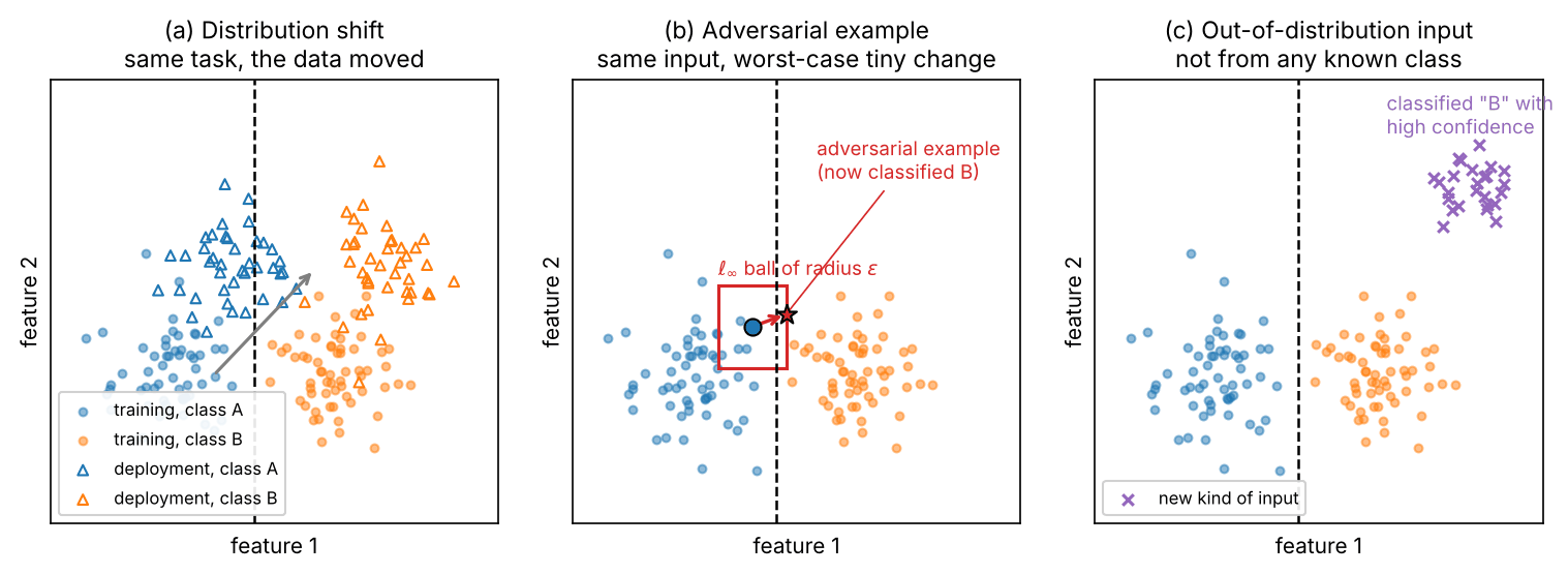
Precise version. Let a classifier be trained on samples from a distribution over images and labels . Write for its accuracy on a distribution .
- Distribution shift. Test data come from , but the label set is the same. The question is how much falls below , and how to reduce the fall.
- Adversarial robustness. For each test pair , an adversary may replace by any in an allowed set , usually a small ball around . The model is robust at if for every . The question is about the worst case, not the average.
- OOD and anomaly detection. Some test inputs have no correct label in (a new object category), or come from a region of input space the training data never covered (a defective part, a corrupted frame). We want a score that is high for in-distribution (ID) inputs and low for these, so that the system can abstain or raise an alarm.
| Distribution shift | Adversarial example | OOD / anomaly | |
|---|---|---|---|
| What changed | the data distribution | one input, on purpose | the input is outside the task |
| Who causes it | the world (camera, place, time) | an adversary with a goal | the world (new classes, defects) |
| What we want | keep accuracy | keep the label under every allowed change | flag the input, do not answer |
| Typical metric | accuracy on shifted test sets | robust accuracy at a budget | AUROC, FPR at 95% TPR |
| In this chapter | Distribution shift | Adversarial examples | OOD and anomaly detection |
The three overlap at the edges. A heavy corruption can make an input effectively OOD; an adversarial example is a shift chosen by an opponent; and ImageNet-A, a set of natural photos selected because they fool a classifier [1], sits between shift and adversarial examples. Still, the table shows why one robustness number can never cover all three: they ask different questions and need different test data.
Distribution shift
Plain version. A familiar task can arrive through new cameras, lighting, styles or locations. Accuracy and confidence may change differently under that shift.
Kinds of shift
The usual vocabulary splits the joint distribution in two ways, , and names the shift by which factor changes:
- Covariate shift: changes, does not. A new scanner, fog, a different hospital’s staining.
- Label (prior) shift: changes, does not. A rare disease becomes common during an outbreak.
- Concept shift: itself changes. The definition of a class is revised.
ML 11 develops these with importance weights and the label-shift correction, so we do not repeat them. Two more terms are common in vision. Domain shift is covariate shift between named data sources (synthetic versus real, one hospital versus another), and subpopulation shift keeps the same kinds of images but changes how often each group appears; WILDS contains both [2]. The survey by Yang et al. adds a distinction that becomes important later in this chapter: a covariate shift changes how inputs look while the labels stay valid, whereas a semantic shift introduces inputs whose labels are outside [3]. We want models to be robust to covariate shift and to detect semantic shift.
Benchmarks that measure robustness to shift
Plain version. Because the real deployment data are rarely available in advance, researchers built test sets that change one thing at a time, or that collect naturally different photos of the same classes.
The main families, all labelled with ImageNet classes unless noted:
- Synthetic corruptions. ImageNet-C applies noise, blur, weather and digital corruptions at five severities, and its authors also proposed ImageNet-P for perturbation sequences [4]. The details and the mean corruption error are in DLCV 02.
- Renditions and style. ImageNet-R collects art, cartoons, sculptures and other renditions; the same paper introduced further real-world shift datasets and found that methods that helped with texture and local image statistics did not help with others, such as geographic change [5].
- Natural adversarial images. ImageNet-A keeps unmodified photos that a ResNet-50 got wrong; they transfer to other models, showing shared weaknesses [1].
- Controlled collection. ObjectNet photographs objects with randomized backgrounds, rotations and viewpoints, as a test set only, with no training split [6].
- Re-collection. ImageNetV2 rebuilt the test set by following the original collection process; accuracy dropped although the procedure was copied as closely as possible [7] (see ML 11).
- In the wild. WILDS gathers ten datasets with shifts that arose in real applications, such as tissue slides from different hospitals and camera traps at new locations, and reports that standard training gives much lower out-of-distribution than in-distribution performance, with existing robustness methods not closing the gap [2].
How to read the numbers. A model with higher clean accuracy usually also has higher shifted accuracy, so “it scores better on ImageNet-R” may only mean “it is a better model”. Taori et al. evaluated 204 ImageNet models in 213 test conditions and proposed effective robustness: accuracy on the shifted set beyond what a fitted trend over standard models predicts from the clean accuracy [8]. Miller et al. found that, for many shifts, shifted and clean accuracy lie close to a straight line across architectures and training choices (“accuracy on the line”), with weaker correlation for some synthetic shifts and for one medical dataset [9]. The consequence for practice: compare robustness interventions at matched clean accuracy, or report both numbers side by side.
Optional: Effective robustness and accuracy on the line (in the Supplementary notes). How the baseline trend is fitted, why logit or probit axes are used, and how to read a robustness scatter plot.
Code: corruptions, augmentation and test-time normalization
The toy trains a small MLP on scikit-learn’s 8×8 digits and corrupts the test images with three corruptions at severities 1 to 5. The network standardizes each pixel with statistics computed on the training set, the way a batch-normalization layer uses running statistics at test time. We compare three models: the plain one; one trained with noise augmentation (a copy of every training image with random-severity noise); and the plain model with test-batch normalization, which recomputes the per-pixel mean and standard deviation on the corrupted test batch instead of using the training statistics.
Code · Python · 36 lines
import numpy as np
from scipy.ndimage import gaussian_filter
from sklearn.datasets import load_digits
from sklearn.model_selection import train_test_split
from sklearn.neural_network import MLPClassifier

X, y = load_digits(return_X_y=True)
X = X / 16.0                                          # 8x8 images, pixels in [0, 1]
Xtr, Xte, ytr, yte = train_test_split(X, y, test_size=0.3, stratify=y, random_state=0)
rng = np.random.default_rng(0)

corruptions = {                                       # severity s = 1..5
    "noise":    lambda X, s: np.clip(X + rng.normal(0, 0.1 * s, X.shape), 0, 1),
    "blur":     lambda X, s: gaussian_filter(X.reshape(-1, 8, 8), (0, 0.25 * s, 0.25 * s)).reshape(-1, 64),
    "contrast": lambda X, s: 0.5 + (X - 0.5) * (1 - 0.15 * s),
}

def norm(X, ref):                                     # standardize each pixel with ref's statistics
    return (X - ref.mean(0)) / (ref.std(0) + 0.05)

def fit(X, y):
    return MLPClassifier(hidden_layer_sizes=(64,), alpha=1e-3, max_iter=400, random_state=0).fit(norm(X, Xtr), y)

plain = fit(Xtr, ytr)
s_rand = rng.integers(1, 6, (len(Xtr), 1))            # random noise severity per training image
augmented = fit(np.vstack([Xtr, corruptions["noise"](Xtr, s_rand)]), np.r_[ytr, ytr])

for name, corrupt in corruptions.items():
    rows = {"plain": [], "noise-aug": [], "test-norm": []}
    for s in range(6):
        Xs = Xte if s == 0 else corrupt(Xte, s)
        rows["plain"].append(plain.score(norm(Xs, Xtr), yte))
        rows["noise-aug"].append(augmented.score(norm(Xs, Xtr), yte))
        rows["test-norm"].append(plain.score(norm(Xs, Xs), yte))   # statistics of the test batch
    for k, v in rows.items():
        print(f"{name:8s} {k:9s}", " ".join(f"{a:.2f}" for a in v))
It prints the test accuracy at severities 0 (clean) to 5:
Code · 9 lines
noise    plain     0.98 0.94 0.75 0.54 0.41 0.31
noise    noise-aug 0.97 0.96 0.93 0.82 0.74 0.62
noise    test-norm 0.98 0.97 0.90 0.83 0.73 0.61
blur     plain     0.98 0.98 0.96 0.82 0.46 0.21
blur     noise-aug 0.97 0.97 0.97 0.90 0.78 0.58
blur     test-norm 0.98 0.98 0.97 0.95 0.89 0.81
contrast plain     0.98 0.92 0.46 0.20 0.19 0.19
contrast noise-aug 0.97 0.98 0.96 0.93 0.84 0.60
contrast test-norm 0.98 0.98 0.98 0.98 0.98 0.98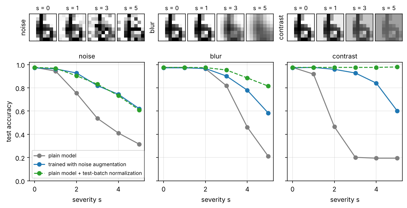
(All numbers are from our toy run.) Four lessons carry over to real networks:
- Mild-looking changes are enough. A contrast reduction to 70% of the original range (severity 2) halves the plain model’s accuracy, although a person reads the digits easily.
- Augmentation helps, and not only for the corruption it used. Training with noise also helped with blur and contrast here, which is the hope behind diverse augmentation. It cost a little clean accuracy (0.98 to 0.97), and real benchmarks show that the transfer to other shifts is far from guaranteed [5], [8].
- Re-estimating normalization statistics is a cheap and strong fix when its assumption holds. The contrast corruption is an affine change of every pixel, which per-pixel standardization undoes exactly, so accuracy stays at 0.98. Noise changes the statistics in a way standardization cannot undo, so the gain is smaller.
- Test-batch normalization needs a batch. It used all 540 test images of one corruption at once. With a few images, or with a batch that mixes several conditions, the statistics are wrong (Exercise 1).
What helps, and what does not
Plain version. Interventions include diverse training, broader pretraining, test-time adaptation, target-domain adaptation and multi-domain training. Choose according to available data and deployment constraints.
Data augmentation. Augmentation makes the training distribution wider so that the test distribution is more likely to fall inside it. AugMix mixes several chains of random augmentations of one image, and adds a Jensen–Shannon consistency loss that asks the network to give similar predictions for the original and the augmented versions [10]. Its authors deliberately removed operations that overlap with ImageNet-C corruptions, so the benchmark measures transfer to unseen corruptions rather than memorization of the test corruptions [10]. Stylized training, which replaces image textures with painting styles, made a ResNet-50 rely more on shape and improved robustness to many distortions [11]. The caution comes from the ImageNet-R study: augmentation and larger models helped on some real-world shifts (style, blur) but not on others (geography), and no evaluated method consistently improved robustness across all of them [5]. General augmentation recipes are in DLCV 02.
Pre-training on more diverse data. In the testbed of Taori et al., most robustness interventions gave little or no effective robustness on natural shifts; the main exception was training on larger and more diverse data [8]. Zero-shot CLIP models, trained on image–text pairs from the web, improved effective robustness by a large amount on natural ImageNet shifts, but the CLIP paper also showed that the benefit almost vanished when a classifier was fitted on ImageNet in a fully supervised way [12]. Fang et al. tested five possible causes (dataset size, training distribution, language supervision during training, language supervision at test time, contrastive loss) and found that the more diverse training distribution was the main cause [13]. Fine-tuning can therefore erode robustness; WiSE-FT averages the weights of the zero-shot and fine-tuned models to keep most of both [14] (see also LP-FT in ML 10).
Test-time adaptation (TTA). If unlabeled test images arrive in batches, the model can adjust itself before predicting. The simplest form is the one in our toy: Schneider et al. replaced the batch-normalization statistics of 25 pretrained models with statistics of the corrupted test images and improved corruption robustness consistently, even when adapting with a single sample [15]. TENT goes one step further: it re-estimates the normalization statistics and updates the channel-wise affine parameters of the normalization layers online, by minimizing the entropy of the model’s own predictions on each test batch [16]. TTA assumes a stream of test data from a reasonably stable shift; it adds computation at test time and can drift if the stream changes.
Optional: Test-time entropy minimization (in the Supplementary notes). The TENT objective, which parameters it changes and why, and the failure cases to watch for.
Unsupervised domain adaptation (UDA). If unlabeled images from the target domain are available during training, the model can be trained to work there without target labels. Domain-adversarial training (DANN) adds a small domain classifier on top of the features and a gradient-reversal layer between them, so that the features become good for the label task on the labelled source domain and, at the same time, useless for telling source from target [17]. The idea rests on domain-adaptation theory: if a classifier cannot tell the domains apart in feature space, a good source classifier should transfer.
Optional: Domain-adversarial training and the gradient-reversal layer (in the Supplementary notes). The DANN objective as a min-max problem, the layer that implements it in one line, and when aligning features hurts.
Domain generalization (DG). Without any target data, the model is trained on several source domains in the hope that it works on an unseen one. The survey by Zhou et al. groups DG methods into domain alignment, meta-learning, data augmentation and ensemble learning, among others [18]. Gulrajani and Lopez-Paz then reran many DG algorithms in one testbed, DomainBed, with equal tuning effort and explicit model-selection rules, and found that plain empirical risk minimization (ERM, ordinary training on the pooled sources) with a strong network and augmentation matched or beat them [19]. Their key point is methodological: a DG method is incomplete without a rule for choosing hyperparameters that does not peek at the test domain.
Optional: Gulrajani and Lopez-Paz, “In Search of Lost Domain Generalization” (in the Paper guides). How DomainBed’s three model-selection rules work and how to read its tables.
What does not help, or not reliably. Robustness on synthetic corruptions was only weakly predictive of robustness on natural shifts in the testbed of Taori et al., and the same held for adversarial robustness [8]. A method tuned on one benchmark often helps only that benchmark [5]. Architecture changes at fixed data have mattered less than the data itself [8], [13]. The practical rule follows: test on several kinds of shift, including at least one real shift from your own deployment.
Confidence under shift
Plain version. Under shift, a model is wrong more often, but it is usually not less confident by the same amount, so its probabilities stop meaning what they say.
Ovadia et al. benchmarked uncertainty methods under dataset shift on several tasks and found that calibration degrades as shift grows, that post-hoc calibration such as temperature scaling fitted on in-distribution validation data falls short under shift, and that methods that average over several models (such as deep ensembles) held up best [20]. Temperature scaling is explained in DLCV 02, and ML 11 shows on a toy how a fitted temperature stops working under shift. The practical consequence: a confidence threshold chosen on clean validation data will accept more wrong answers in the field, so monitor the distribution of confidences after deployment (ML 11).
Adversarial examples
Plain version. For almost any correctly classified image, there is a nearby image, often indistinguishable to a person, that the network classifies wrongly. An attacker finds it by asking the network itself which direction to move each pixel.
What an adversarial example is
Szegedy et al. reported that deep networks can be made to misclassify an image by an imperceptible perturbation found by maximizing the network’s prediction error, and that the same perturbation often fools a different network trained on a different subset of the data [21]. Goodfellow et al. explained the effect by the near-linearity of networks in high dimensions and introduced the one-step fast gradient sign method [22], which DLCV 02 derives and tests. This section adds the parts needed to evaluate and improve robustness: threat models, the multi-step attack, adversarial training, honest evaluation and certificates.
Threat models
Plain version. “Robust” means nothing until you say robust to what: how much may the attacker change, and what does the attacker know?
A threat model fixes three things.
1. The allowed perturbations. Most work uses an ball of radius around the clean image :
where is the number of pixel values, is the perturbation and its -th entry. The ball lets every pixel change by at most (a small change everywhere); the ball bounds the total energy of the change; the “norm” counts how many pixels change (a few pixels, changed a lot). On CIFAR-10, in is a standard budget: Madry et al. trained and attacked with on the 0–255 pixel scale [23], and RobustBench keeps leaderboards for and threat models and for common corruptions [24]. A small norm is a convenient proxy for “imperceptible”, not a definition of it.
2. The attacker’s knowledge. In a white-box attack, the attacker knows the model and its weights and can compute gradients. In a black-box attack, the attacker only queries the model. Papernot et al. showed a practical black-box attack: label inputs by querying the target model, train a local substitute model on them, craft adversarial examples on the substitute, and rely on transfer to the target [25]. Other black-box attacks estimate the decision boundary from queries alone. Robustness claims should be made against white-box attacks, because what one attacker cannot do today, a better-informed one may do tomorrow.
3. The goal. An untargeted attack wants any wrong label; a targeted attack wants a specific one (a stop sign read as a speed limit). Targeted attacks are harder, so the two give different numbers.
FGSM and PGD, precisely
Plain version. FGSM takes one big step uphill on the loss. PGD takes many small steps uphill and, after each step, pulls the image back into the allowed ball. PGD finds stronger adversarial examples and is the standard first-order attack.
Let be the cross-entropy loss of the network with parameters on input with label . FGSM [22] for the ball is
where is the gradient of the loss with respect to the input pixels, is applied to each entry (giving , or ), and clips each pixel to the valid range. Moving every pixel by exactly in the direction that increases the loss is the best a linear approximation of the loss can do inside the ball.
Projected gradient descent (PGD) [23] repeats a smaller step times, starting from a random point in the ball:
where is uniform noise in the ball (the random start), is the step size, counts the steps, and is the projection onto the allowed set. For the ball intersected with the valid pixel range, the projection is two clips: first , then . The final iterate is the adversarial example. PGD is “gradient ascent on the loss”; the name comes from optimization, where the same algorithm minimizes. Because the loss surface is not concave, the random start and a few restarts help; Madry et al. observed that the losses reached from many random starts were well concentrated, which supported PGD as a reliable first-order adversary [23].
A second common loss is the margin loss of Carlini and Wagner, which directly maximizes the gap between the largest wrong logit and the correct logit instead of the cross-entropy [26]. It matters when the cross-entropy saturates, and it is one reason a serious evaluation runs several attacks.
Optional: Attack settings that decide an evaluation (in the Supplementary notes). Step size, number of steps, restarts, the margin loss, PGD, and what AutoAttack fixes.
Adversarial training
Plain version. If the model fails on the worst nearby image, train it on the worst nearby image. During training, attack every batch with PGD and fit the attacked images instead of the clean ones.
Madry et al. wrote robust training as a min-max (saddle point) problem [23]:
where is the data distribution, the set of allowed perturbations (for example, ), the inner maximum is the attacker’s best perturbation and the outer minimum is the defender’s training. In practice, the inner maximum is approximated by PGD with a few steps and the outer minimum by ordinary stochastic gradient descent on the resulting adversarial batch.
What it costs:
- Compute. Every training step needs a -step attack, so training is roughly times as expensive.
- Capacity. Madry et al. found that robust classification needs larger networks than clean classification; small networks trained against PGD could collapse to predicting one class, and training against one-step FGSM overfitted to its narrow set of perturbations and did not give robustness to PGD at large [23].
- Clean accuracy. Robust models are usually less accurate on clean data. Tsipras et al. proved that this trade-off exists in a simple, natural setting and argued that robust models learn different features, which happen to align better with human perception [27]. TRADES splits the robust error into the natural error plus a boundary error and trains with a loss that trades the two explicitly through one weight [28].
Optional: Madry et al., “Towards Deep Learning Models Resistant to Adversarial Attacks” (in the Paper guides). The saddle-point view, the capacity experiments and how to read its attack tables.
Code: FGSM, PGD and adversarial training on digits
NumPy computes the input gradient of a one-hidden-layer MLP by hand: for softmax outputs and a one-hot label , the gradient of the cross-entropy with respect to the logits is , which we pass back through the output layer, the ReLU and the first layer. Both models get the same 50 passes over the training data; the robust one is fitted on PGD examples (, 5 steps) made against its current weights.
Code · Python · 42 lines
import numpy as np
from sklearn.datasets import load_digits
from sklearn.model_selection import train_test_split
from sklearn.neural_network import MLPClassifier

X, y = load_digits(return_X_y=True)
X = X / 16.0                                          # pixels in [0, 1]
Xtr, Xte, ytr, yte = train_test_split(X, y, test_size=0.3, stratify=y, random_state=0)
rng = np.random.default_rng(0)

def input_grad(m, X, y):
    """Gradient of the cross-entropy loss with respect to the input pixels."""
    (W1, W2), (b1, b2) = m.coefs_, m.intercepts_
    h = np.maximum(X @ W1 + b1, 0)                    # hidden ReLU layer
    z = h @ W2 + b2                                   # logits
    g = np.exp(z - z.max(1, keepdims=True)); g /= g.sum(1, keepdims=True)
    g[np.arange(len(y)), y] -= 1                      # dL/dz = softmax(z) - one-hot(y)
    return ((g @ W2.T) * (h > 0)) @ W1.T              # back through ReLU and first layer

def fgsm(m, X, y, eps):
    return np.clip(X + eps * np.sign(input_grad(m, X, y)), 0, 1)

def pgd(m, X, y, eps, steps=10):
    alpha = 2.5 * eps / steps                         # step size
    Xa = np.clip(X + rng.uniform(-eps, eps, X.shape), 0, 1)        # random start in the ball
    for _ in range(steps):
        Xa = Xa + alpha * np.sign(input_grad(m, Xa, y))             # ascent step on the loss
        Xa = np.clip(np.clip(Xa, X - eps, X + eps), 0, 1)           # project: eps-ball, then [0, 1]
    return Xa

def train(adversarial, epochs=50, eps=0.15):
    m = MLPClassifier(hidden_layer_sizes=(128,), random_state=0)
    m.partial_fit(Xtr, ytr, classes=np.arange(10))    # first pass on clean images
    for _ in range(epochs - 1):                       # Madry et al.: fit the worst case found by PGD
        m.partial_fit(pgd(m, Xtr, ytr, eps, steps=5) if adversarial else Xtr, ytr)
    return m

standard, robust = train(False), train(True)
for eps in [0, 0.05, 0.1, 0.15, 0.2]:
    acc = [m.score(atk(m, Xte, yte, eps), yte) for m in (standard, robust) for atk in (fgsm, pgd)]
    print(f"eps={eps:.2f}  standard: FGSM {acc[0]:.3f} PGD {acc[1]:.3f}"
          f"   adversarially trained: FGSM {acc[2]:.3f} PGD {acc[3]:.3f}")
It prints (about 10–20 seconds on a laptop CPU):
Code · 5 lines
eps=0.00  standard: FGSM 0.967 PGD 0.967   adversarially trained: FGSM 0.956 PGD 0.956
eps=0.05  standard: FGSM 0.861 PGD 0.854   adversarially trained: FGSM 0.891 PGD 0.889
eps=0.10  standard: FGSM 0.574 PGD 0.528   adversarially trained: FGSM 0.757 PGD 0.746
eps=0.15  standard: FGSM 0.237 PGD 0.178   adversarially trained: FGSM 0.626 PGD 0.593
eps=0.20  standard: FGSM 0.057 PGD 0.007   adversarially trained: FGSM 0.415 PGD 0.361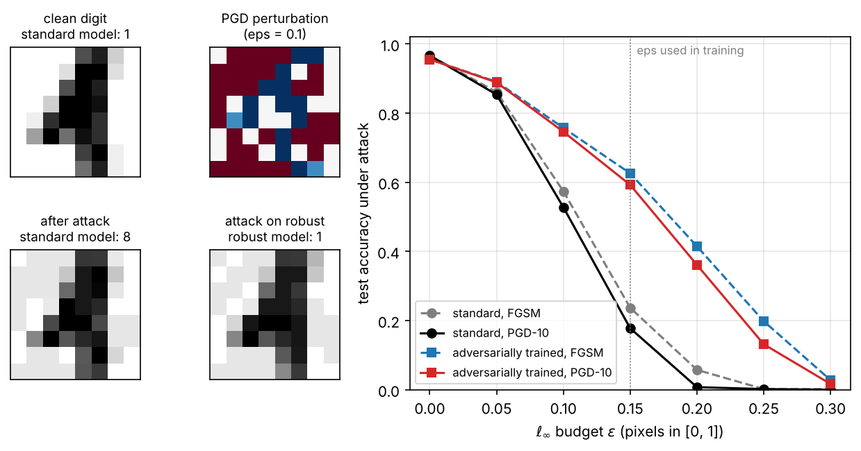
(All numbers are from our toy run.) Read the table in three directions:
- Down a column: accuracy falls quickly with . At , each pixel may change by 1.6 of the dataset’s 16 gray levels, and the standard model drops from 0.967 to 0.528 under PGD.
- Across an attack pair: PGD is never weaker than FGSM, and the gap grows with (0.057 versus 0.007 at for the standard model). An evaluation with FGSM alone overstates robustness.
- Across models: adversarial training raises PGD accuracy at from 0.178 to 0.593, and costs about one point of clean accuracy (0.967 to 0.956), a small version of the trade-off. Beyond the training budget, robustness fades (0.131 at in the figure): robustness is guaranteed for nothing outside the threat model it was trained for.
Evaluating robustness honestly
Plain version. It is easy to build a “defense” that only breaks the attacker’s tools, for example by making gradients useless, while the model stays just as easy to fool. The robustness then exists only on paper, until someone uses a better attack.
Athalye, Carlini and Wagner named this obfuscated gradients, a kind of gradient masking, and described three types [29]: shattered gradients (non-differentiable or numerically unstable operations, such as quantizing the input, give gradients that are zero or wrong); stochastic gradients (random input transformations at test time make a single gradient misleading); and vanishing or exploding gradients (defenses that run an iterative procedure, such as projecting the input onto a learned manifold, behave like an extremely deep network). For each type they gave a counter-attack: BPDA (backward pass differentiable approximation) runs the defense normally in the forward pass but replaces it by a differentiable approximation, often the identity, in the backward pass; EOT (expectation over transformation) averages gradients over the random transformations; and reparameterization changes variables so that the iterative step disappears from the gradient path. In a case study of nine white-box defenses accepted at ICLR 2018, seven relied on obfuscated gradients, and their attacks fully circumvented six and partially one [29].
The same paper lists warning signs that an evaluation is broken: one-step attacks work better than iterative ones; black-box attacks work better than white-box ones; unbounded attacks do not reach 100% success; random sampling finds adversarial examples that gradient attacks miss; and increasing the budget does not increase success [29]. Our toy passes the checks it can: PGD beats FGSM, and accuracy reaches zero as grows.
To make evaluations less dependent on the evaluator’s care, Croce and Hein proposed AutoAttack, a parameter-free ensemble of two improved PGD variants (with an automatic step-size schedule and a different loss) and two complementary existing attacks; applied to over 50 published defenses, it gave lower robust accuracy than reported in all but one case [30]. RobustBench builds a public leaderboard on AutoAttack with rules on allowed models, and invites adaptive attacks where AutoAttack may overestimate robustness [24]. A reported robust accuracy should therefore state the threat model, , the attacks (at least AutoAttack or an adaptive attack designed for the defense), the number of steps and restarts, and the test set.
Optional: Athalye et al., “Obfuscated Gradients Give a False Sense of Security” (in the Paper guides). The three types of masking, the attacks that undo them, and what its case-study table shows.
Certified robustness
Plain version. An attack can only show that a model is not robust at a point. A certificate proves that no perturbation within a radius changes the answer, whatever attack is used.
Randomized smoothing [31] was, according to its authors, the only certified defense shown to be feasible on ImageNet at the time, and it remains the standard reference point. Take any base classifier and define a smoothed classifier that returns the class predicts most often under Gaussian noise:
where is isotropic Gaussian noise with standard deviation per pixel and is the identity matrix. Cohen, Rosenfeld and Kolter proved that if the top class has probability at least under the noise and every other class at most , then predicts for every perturbation with
where is the inverse of the standard normal cumulative distribution function [31]. In practice, is a lower confidence bound estimated from Monte Carlo samples, and the method abstains when it cannot certify. The guarantee holds for the threat model, with a chosen failure probability, and for the smoothed classifier , not for . Larger allows larger radii but lowers clean accuracy, the same trade-off in another form.
Optional: Randomized smoothing in practice (in the Supplementary notes). The certification algorithm step by step, why the radius is capped by the number of samples, and a tested NumPy snippet.
Physical and patch attacks
Plain version. An attack does not have to be invisible or digital. A printed sticker can fool a camera.
Eykholt et al. generated perturbations that survive changes of viewpoint, distance and lighting, printed them as black-and-white stickers on a real stop sign, and caused a road-sign classifier to output the attacker’s target class in most lab images and in many frames of a drive-by video [32]. Brown et al. made adversarial patches: universal, printable image regions that, placed anywhere in a scene, make a classifier report a chosen class [33]. Such attacks leave the threat model: they are large but localized. They matter for any camera-based system, and they connect to the presentation attacks on face recognition discussed in DLCV 02A.
Out-of-distribution and anomaly detection
Plain version. A classifier always picks one of its known classes, even for a photo of something it has never seen. OOD detection adds a second output, a score that says “this input looks like my training data” or “it does not”, so the system can refuse to answer.
Which task are you solving?
Several closely related tasks go by different names. Yang et al. place them in one framework, generalized OOD detection, and distinguish them by what kind of shift must be detected and by whether ID data has one class or many [3]:
| Task | In-distribution data | Must flag | Typical example |
|---|---|---|---|
| OOD detection | a -class training set | inputs from other classes (semantic shift), while still classifying ID inputs | a pet classifier sees a car |
| Open-set recognition | known classes | unknown classes, while classifying known ones | PR 10, DLCV 02A |
| Sensory anomaly detection | normal images of one kind | inputs that look different (covariate shift) | a scratched part on a production line |
| Semantic anomaly / novelty detection | one or a few classes | inputs from any other class | a new species in camera-trap images |
OOD detection and open-set recognition differ mainly in their history and benchmarks; the survey treats open-set recognition as multi-class novelty detection [3]. All of them differ from the reject option of PR 01, which abstains on ambiguous inputs between known classes rather than on novel ones.
Scores
Plain version. Each detector boils down to one number per input. Output-based scores ask how confident the classifier is; feature-based scores ask how far the input’s features lie from the training features.
Let be the logits of a trained classifier, its penultimate features (the input to the last linear layer), and adopt the convention that a larger score means more in-distribution. Four standard post-hoc scores, which need no retraining:
Maximum softmax probability (MSP) [34]:
where is the -th logit. Hendrycks and Gimpel showed that correctly classified examples tend to have higher MSP than misclassified and OOD ones, which made MSP the standard baseline [34].
Energy score [35]:
where is a temperature (usually ). The negative energy is a log-sum-exp of the logits, a smooth maximum that keeps the size of the logits, which the softmax normalizes away. Liu et al. argued that energy is better aligned with the input density than the softmax confidence, and reported lower FPR at 95% TPR than MSP on their CIFAR benchmarks [35].
Mahalanobis distance [36]: fit one Gaussian per class to the training features, with class means and one shared (“tied”) covariance , and score
where the minimum runs over the classes. This is the linear discriminant analysis of PR 01 placed on learned features. Lee et al. also added a small input perturbation and combined several layers; we use the last hidden layer only.
k-nearest-neighbour (kNN) distance [37]: normalize features to unit length, , and score
where is the -th nearest normalized training feature to . Sun et al. found that this non-parametric score, with no Gaussian assumption, works well and that feature normalization is critical [37].
These scores leave the classifier unchanged. Training-time methods change it: Outlier Exposure trains the classifier to give uniform (low-confidence) predictions on a large auxiliary set of outlier images, which improved detection of unseen OOD data in the original experiments [38].
Metrics
Plain version. Treat detection as a binary decision, ID versus OOD, and ask how well the score separates the two groups, either over all thresholds or at one threshold that keeps most ID inputs.
Treat ID test inputs as positives and OOD inputs as negatives, and accept an input when . Then is the fraction of ID inputs accepted and the fraction of OOD inputs accepted. Three metrics are standard [35]:
- AUROC, the area under the curve of against as varies. It equals the probability that a random ID input gets a higher score than a random OOD input; 0.5 is chance, 1 is perfect separation.
- FPR@95TPR , where is the threshold with : the fraction of OOD inputs still accepted when 95% of ID inputs are kept. Lower is better. It describes one operating point, the kind a deployed system actually uses.
- AUPR, the area under the precision–recall curve, reported with ID inputs as the positive class (AUPR-In) or with OOD inputs as the positive class (AUPR-Out) [34]. It depends on the ratio of ID to OOD test inputs, which should therefore be reported.
ROC and precision–recall curves themselves are explained in DLCV 02.
Code: four scores, near and far OOD
ID data are the digits 0–4. Near-OOD inputs are the unseen digits 5–9: the same kind of image, new classes. Far-OOD inputs are 8×8 patches of photographs from scikit-image, rescaled to the same pixel range: a different kind of image altogether. The classifier never sees either during training.
Code · Python · 46 lines
import numpy as np
from scipy.special import logsumexp, softmax
from skimage import data, transform
from sklearn.datasets import load_digits
from sklearn.metrics import roc_auc_score
from sklearn.model_selection import train_test_split
from sklearn.neural_network import MLPClassifier

X, y = load_digits(return_X_y=True)
X = X / 16.0
known = y < 5                                         # in-distribution (ID): digits 0-4
Xtr, Xid, ytr, yid = train_test_split(X[known], y[known], test_size=0.3, stratify=y[known], random_state=0)
X_near = X[~known]                                    # near-OOD: unseen digits 5-9
rng = np.random.default_rng(0)
photos = [transform.resize(im / 255.0, (256, 256)) for im in (data.camera(), data.moon(), data.coins(), data.text())]
X_far = []                                            # far-OOD: 8x8 patches of photographs
for _ in range(600):
    im = photos[rng.integers(4)]; r, c = rng.integers(0, 224, 2)
    p = transform.resize(im[r:r + 32, c:c + 32], (8, 8), anti_aliasing=True)
    X_far.append(((p - p.min()) / (np.ptp(p) + 1e-8)).ravel())
X_far = np.array(X_far)

m = MLPClassifier(hidden_layer_sizes=(64,), alpha=1e-3, max_iter=500, random_state=0).fit(Xtr, ytr)
(W1, W2), (b1, b2) = m.coefs_, m.intercepts_
feat = lambda X: np.maximum(X @ W1 + b1, 0)           # penultimate (hidden) features
unit = lambda F: F / (np.linalg.norm(F, axis=1, keepdims=True) + 1e-12)
F = feat(Xtr)
mu = np.stack([F[ytr == c].mean(0) for c in range(5)])           # class means
cov = sum(np.cov(F[ytr == c].T, bias=True) * np.sum(ytr == c) for c in range(5)) / len(F)
P = np.linalg.inv(cov + 1e-3 * np.eye(len(cov)))                # shared precision matrix

def scores(X):                                        # every score: larger = "more in-distribution"
    H = feat(X); z = H @ W2 + b2; d = H[:, None] - mu[None]
    return {"MSP": softmax(z, axis=1).max(1),
            "energy": logsumexp(z, axis=1),           # = -E(x) with temperature 1
            "Mahalanobis": -np.einsum("ncd,de,nce->nc", d, P, d).min(1),
            "kNN": -np.sort(np.linalg.norm(unit(H)[:, None] - unit(F)[None], axis=2), 1)[:, 9]}

s_id = scores(Xid)
print(f"ID test accuracy {m.score(Xid, yid):.3f}")
for name, X_ood in [("near", X_near), ("far", X_far)]:
    s_ood = scores(X_ood)
    for k in s_id:
        auroc = roc_auc_score(np.r_[np.ones(len(Xid)), np.zeros(len(X_ood))], np.r_[s_id[k], s_ood[k]])
        fpr95 = np.mean(s_ood[k] >= np.quantile(s_id[k], 0.05))  # OOD accepted when 95% of ID is kept
        print(f"{name:4s} {k:11s} AUROC {auroc:.3f}  FPR@95TPR {fpr95:.3f}")
It prints:
Code · 9 lines
ID test accuracy 1.000
near MSP         AUROC 0.941  FPR@95TPR 0.291
near energy      AUROC 0.955  FPR@95TPR 0.258
near Mahalanobis AUROC 0.961  FPR@95TPR 0.209
near kNN         AUROC 0.970  FPR@95TPR 0.152
far  MSP         AUROC 0.870  FPR@95TPR 0.448
far  energy      AUROC 0.811  FPR@95TPR 0.660
far  Mahalanobis AUROC 1.000  FPR@95TPR 0.000
far  kNN         AUROC 0.995  FPR@95TPR 0.010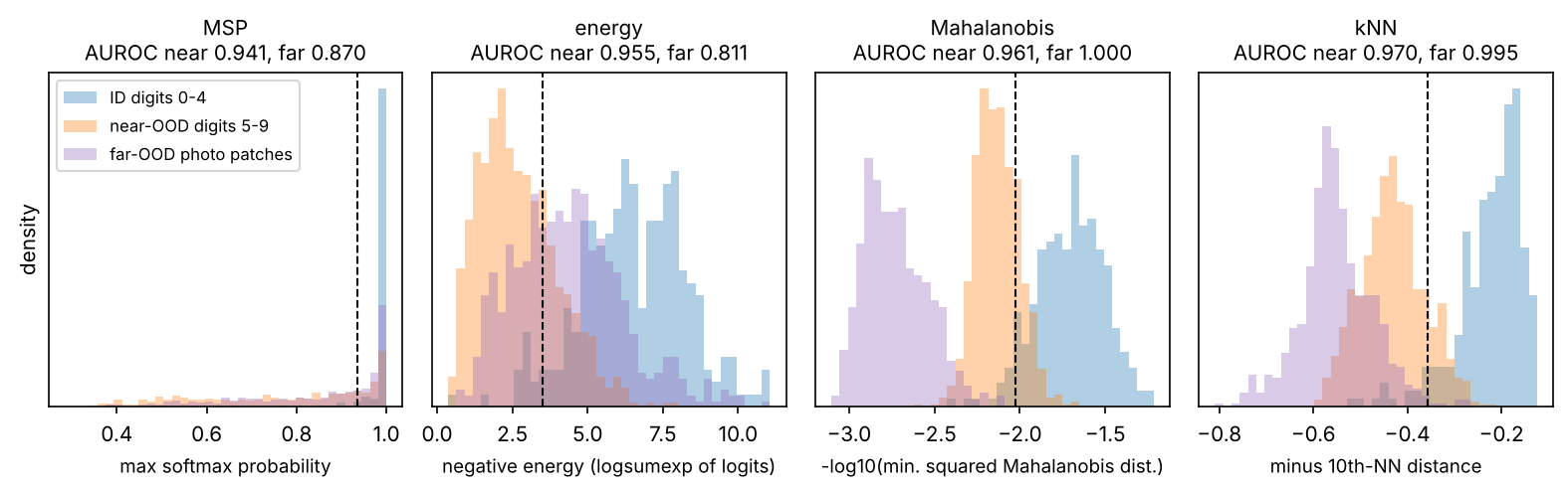
(All numbers are from our toy run.) Three lessons:
- “Far” in content is not “easy” for every score. The photo patches are nothing like digits, yet MSP accepts 45% and energy 66% of them at the 95%-TPR threshold. The classifier maps them confidently onto some digit, because confidence measures distance from the decision boundary, not distance from the data. Feature-distance scores see that the patches’ features are far from all training features and reject almost all of them.
- The ranking of scores changes with the OOD set. Energy beats MSP on the unseen digits but loses to it on the patches. A large benchmark study, OpenOOD v1.5, likewise found no single method that wins across datasets [39].
- AUROC and FPR@95TPR disagree in size. An AUROC of 0.941 sounds good, but at a deployable threshold MSP still accepts 29% of unseen digits.
PR 10 runs a related open-set experiment with held-out digits on a different classifier and shows how a proxy-unknown set can mislead (PR 10).
Industrial anomaly detection
Plain version. On a production line, defects are rare and varied, so you cannot collect examples of every defect. Instead, you learn only what normal parts look like, patch by patch, and flag any patch that looks unlike every normal patch you have seen.
MVTec AD made this setting a standard benchmark: 5354 high-resolution images of object and texture categories, defect-free images for training, test images with more than 70 types of defects (scratches, dents, contaminations, structural changes), and pixel-precise masks of the defect regions [40]. Methods are scored at two levels: image-level (is this part defective?) and pixel-level (where is the defect?), usually with AUROC; region-overlap measures such as AU-PRO are also used, for example by MVTec AD 2 [41]. This is sensory anomaly detection in the terms of the table above.
PatchCore [42] is a strong, simple method built on the kNN idea. It passes defect-free training images through a network pre-trained on ImageNet and keeps mid-level patch features (the last layers are too specific to ImageNet classes and too coarse for small defects), each averaged over a small neighbourhood for context. All these features go into a memory bank, which greedy coreset subsampling shrinks to a small subset that still covers rare normal patterns. At test time, each patch’s distance to its nearest neighbour in the memory bank forms the anomaly map, and the map’s maximum (slightly re-weighted) is the image score. The method was designed for the “cold-start” setting in which only nominal (defect-free) images are available, and it reached state-of-the-art detection and localization on MVTec AD [42].
Optional: PatchCore step by step (in the Supplementary notes). The neighbourhood aggregation, the minimax coreset objective and its greedy solution, and the score re-weighting, with every symbol defined.
Code: a patch memory bank on a brick wall
Without network weights we use raw 7×7 pixel patches as features, which keeps the mechanics of PatchCore (memory bank, coreset, nearest-neighbour distance map, max-pooled image score) and drops the learned features. “Products” are 64×64 crops of scikit-image’s brick-wall texture: normal training crops from the top half of the image, test crops from the bottom half, and half of the test crops receive a thin synthetic scratch.
Code · Python · 43 lines
import numpy as np
from skimage import data, draw, transform
from skimage.util import view_as_windows
from sklearn.metrics import roc_auc_score
from sklearn.neighbors import NearestNeighbors

rng = np.random.default_rng(0)
tex = transform.rescale(data.brick() / 255.0, 0.5)   # 256x256 brick-wall "product surface"
S, P = 64, 7                                          # image size, patch size

def crop(top):                                        # normal images: top half; test images: bottom half
    r = rng.integers(0, 128 - S) + (0 if top else 128); c = rng.integers(0, 256 - S)
    return tex[r:r + S, c:c + S].copy()

def scratch(im):                                      # a thin line, 0.5 brighter or darker
    r, c = rng.integers(16, S - 16, 2); a = rng.uniform(0, np.pi); L = rng.integers(8, 16)
    rr, cc = draw.line(r, c, int(r + L * np.sin(a)), int(c + L * np.cos(a)))
    mask = np.zeros_like(im, bool); mask[rr, cc] = True
    im[mask] = np.clip(im[mask] + rng.choice([-0.5, 0.5]), 0, 1)
    return im, mask

def patches(im, step=1):                              # one 7x7 patch centred on each pixel
    return view_as_windows(np.pad(im, P // 2, mode="reflect"), (P, P), step).reshape(-1, P * P)

def greedy_coreset(M, n):                             # keep n patches that cover the bank well
    keep, d = [0], np.linalg.norm(M - M[0], axis=1)
    for _ in range(n - 1):
        i = int(d.argmax()); keep.append(i)
        d = np.minimum(d, np.linalg.norm(M - M[i], axis=1))
    return M[keep]

bank = np.vstack([patches(crop(top=True), step=2) for _ in range(16)])
memory = NearestNeighbors(n_neighbors=1).fit(greedy_coreset(bank, len(bank) // 10))

is_defect, img_score, pix_score, pix_true = [], [], [], []
for k in range(40):
    im, mask = scratch(crop(top=False)) if k % 2 else (crop(top=False), np.zeros((S, S), bool))
    amap = memory.kneighbors(patches(im))[0].reshape(S, S)   # nearest-neighbour distance per pixel
    is_defect.append(k % 2); img_score.append(amap.max())
    pix_score.append(amap.ravel()); pix_true.append(mask.ravel())
print(f"memory bank {len(bank)} -> {len(bank) // 10} patches")
print(f"image-level AUROC {roc_auc_score(is_defect, img_score):.3f}")
print(f"pixel-level AUROC {roc_auc_score(np.concatenate(pix_true), np.concatenate(pix_score)):.3f}")
It prints:
Code · 3 lines
memory bank 16384 -> 1638 patches
image-level AUROC 0.955
pixel-level AUROC 0.996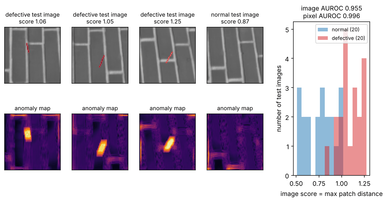
(All numbers are from our toy run.) The pixel-level AUROC is almost perfect, but the image-level AUROC is lower: one image score is the maximum over 4096 patch distances, so a single unusual but normal patch (a mortar corner that the memory bank lacks) raises a normal image’s score as much as a real defect does. More normal training images reduce such false alarms; fainter defects increase them (Exercise 4). In the anomaly maps, mortar edges glow a little: they are the rarest normal structures, which is exactly why PatchCore keeps a coreset that covers them instead of a random subsample.
Pitfalls in OOD and anomaly evaluation
Plain version. OOD numbers depend more on which OOD data was chosen than on the method, and many published OOD test sets are flawed. Read every OOD result together with its test sets.
- Near- versus far-OOD. OpenOOD groups OOD test sets into near-OOD (similar to the ID data) and far-OOD (clearly different), and finds a large gap in detection performance between the two groups for all detectors [39]. Our toy shows that the label can mislead: for output-based scores, “far” photo patches were harder than “near” digits.
- Contaminated OOD test sets. Bitterwolf et al. found that many OOD test sets used with ImageNet-1K contain a large share of images that actually show ID classes, in some cases more than half, which distorts the evaluation; they built NINCO, an OOD test set with every image checked to be free of ID objects [43].
- Pre-training overlap. A detector built on a model pre-trained on web-scale data may have seen the “unknown” classes during pre-training. Then the test is no longer about the unknown, and the setting must be described accordingly.
- Thresholds and model selection. Like any hyperparameter, the threshold and the choice of score must be set on validation data. Tuning them on the OOD test set (or on a proxy that is too similar to it) gives the same optimism as the oracle model selection that DomainBed warns against [19].
- Covariate shift inside the ID set. In deployment, an ID image may arrive blurred or under new lighting. OpenOOD v1.5 evaluates “full-spectrum” detection, in which covariate-shifted ID images must be accepted while semantic OOD images are rejected, and finds it a significant challenge for all current approaches [39]. This is where the first and third problems of this chapter meet.
A robustness evaluation plan
Plain version. Before claiming a model is robust, write down what it is robust to, test that with the strongest tools available, and report the result next to the clean number.
- Name the problem. Shift (which kind?), adversary (which threat model?), or unknown inputs (which kind of novelty?). If several, evaluate each separately.
- Build the test data first. At least one real shifted set from the expected deployment (new site, device or time), synthetic corruptions as a cheap supplement, and a held-out OOD set that is checked for ID contamination.
- Use strong evaluation. For adversarial claims: white-box attacks, PGD with restarts and AutoAttack or an adaptive attack, the warning-sign checks above, and the exact and norm. For shift: effective robustness or matched clean accuracy. For OOD: AUROC and FPR@95TPR on near- and far-OOD sets.
- Keep the test data out of the loop. Choose hyperparameters, thresholds and checkpoints on validation data from the training distribution, or state clearly that an oracle was used.
- Report the trade-offs. Clean accuracy, robust accuracy, calibration, and compute cost together; a gain in one is not free.
- Monitor after release. Track input statistics and confidence distributions, as in ML 11, and in multi-sensor systems the sensor faults listed in DLCV 03B.
Modern view
Surveys worth reading.
- Yang, Zhou, Li and Liu [3] (IJCV 2024) unify anomaly detection, novelty detection, open-set recognition, OOD detection and outlier detection as sub-tasks of generalized OOD detection, organized by whether covariate or semantic shift must be detected and by whether ID data has one or several classes; they then review each area, with most detail on OOD detection methods (classification-based, density-based and distance-based). Read it first to sort out the vocabulary.
- Zhou et al. [18] (TPAMI) define domain generalization, relate it to domain adaptation and transfer learning, and review methods grouped into domain alignment, meta-learning, data augmentation, ensemble learning and others, together with theory and applications beyond vision.
- Liang, He and Tan [44] (IJCV) categorize test-time adaptation by the form of test data into test-time domain adaptation, test-time batch adaptation and online test-time adaptation, with a taxonomy of algorithms in each group and a discussion of open challenges.
- Akhtar, Mian, Kardan and Shah [45] (IEEE Access 2021) review adversarial attacks and defenses in computer vision since 2018: attacks on classifiers, attacks beyond classification, physical-world attacks, theories of why adversarial examples exist, and defenses grouped into model modification, input modification and external detectors, with certified defenses treated separately.
- Pang, Shen, Cao and van den Hengel [46] (ACM Computing Surveys 2021) organize deep anomaly detection into three frameworks: deep learning for generic feature extraction, learning representations of normality, and end-to-end anomaly score learning, with eleven finer categories, and discuss each one’s assumptions, advantages and disadvantages.
- Liu et al. [47] (Machine Intelligence Research 2024) review industrial image anomaly detection by network architecture, level of supervision, loss function, metrics and datasets, and propose a setting closer to real manufacturing.
The takeaways they share. Distribution shift, adversarial robustness and OOD detection grew as separate communities with separate benchmarks, and the surveys repeatedly find that benchmark choice, model selection and evaluation protocol drive results as much as methods do. Simple baselines (ERM with good training, MSP or kNN scores, adversarial training with PGD) remain hard to beat when compared fairly.
State of the art, 2023–2026. Five trends are visible. (1) Foundation models changed the starting point. Large, diverse pre-training gives much of the natural-shift robustness that specialized methods could not [12], [13], and robust fine-tuning such as weight interpolation tries to keep it [14]; OOD benchmarks now include CLIP and DINOv2 backbones [39]. (2) Generated data for adversarial training. Training on images from a modern diffusion model, without external real data, set new results on RobustBench for CIFAR-10 and CIFAR-100 [48]; robust accuracy on these benchmarks still lies far below clean accuracy. (3) Better OOD evaluation. Unified benchmarks with near- and far-OOD splits and full-spectrum settings [49], [39] and cleaned test sets [43] replaced ad hoc comparisons. (4) Zero- and few-shot anomaly detection. WinCLIP uses CLIP with prompt ensembles over state words and window-level features to classify and segment anomalies with no or very few normal images [50]. (5) Harder industrial benchmarks. Because results on MVTec AD saturated, MVTec AD 2 adds transparent and overlapping objects, unusual illumination, high variance of normal data, very small defects and test scenarios with lighting changes, and reports that state-of-the-art methods remain far from solving it [41].
Open problems. Robustness to natural shifts that no benchmark anticipated; adversarial robustness beyond small balls (patches, physical changes, semantic edits) and at the scale of foundation models; certificates that are tight at useful radii for large images; OOD detection when the backbone may have seen everything during pre-training; detectors that accept covariate-shifted ID inputs while rejecting semantic novelty; and a common evaluation protocol that tests all three problems of this chapter on the same model.
Key takeaways
- Shift, adversarial robustness and OOD detection require different test conditions and metrics.
- State available target data before comparing adaptation with generalization.
- Adversarial claims require a threat model, attack access and perturbation budget.
- Strong or adaptive attacks help expose gradient masking; certificates cover only their stated assumptions.
- Evaluate OOD scores on multiple near/far sets and check contamination; no score is universally best.
- For anomaly detection, distinguish image-level decisions from localization and verify the normal-data assumptions.
- Compare clean performance, robustness, operating thresholds and cost under one explicit protocol.
Exercises
- Test-batch normalization with small or mixed batches. In the corruption snippet, apply test-batch normalization to batches of 8 test images instead of all 540, and then to one batch that mixes all three corruptions at severity 3. How does accuracy change, compared with the plain model and the noise-augmented one? What does this say about deploying test-time adaptation on a camera that switches between day and night?
Hint
Split Xs into chunks with np.array_split(Xs, len(Xs) // 8), normalize each chunk with its own statistics, and concatenate the predictions. In our run at severity 3, batches of 8 kept part of the gain (noise: 0.86 with the full batch, 0.74 with batches of 8, 0.56 for the plain model; blur: 0.95, 0.87, 0.82). A batch mixing the three corruptions still helped here (0.91 against 0.55 for the plain model), because all three corruptions change the per-pixel statistics in a similar direction (less contrast, more spread); do not expect that in general. Small batches give noisy statistics, and a batch that mixes very different conditions (day and night) gives statistics that fit neither, so real TTA methods need reasonably large batches from one condition, or a way to detect a change in the stream and reset.
- A defense that only breaks the gradient. Add a “defense” to the adversarial snippet that rounds every input pixel to the nearest multiple of 0.25 before the standard model sees it, and recompute the input gradient through the rounding (it is zero almost everywhere). What do FGSM and PGD report? Then attack again with BPDA, treating the rounding as the identity in the backward pass only. Which warning signs from the evaluation section did the first result show?
Hint
With a zero gradient, np.sign returns zeros and PGD never moves from its random start. In our run the “defended” model kept 0.96 accuracy under this PGD at , while random sign noise did better as an attack (0.93): random sampling beating a gradient attack is one of the warning signs. With BPDA, use input_grad(m, quantize(Xa), y) as the gradient at Xa. At the attack is weaker than on the undefended model (0.79 against 0.53), because rounding to steps of 0.25 undoes perturbations smaller than half a step; at BPDA drives accuracy to 0.01, below the undefended model’s 0.18. This is the shattered-gradient case of Athalye et al.
- Accuracy–robustness trade-off. Train the robust model with training budgets and plot clean accuracy against PGD accuracy at . Where is the knee of the curve? What changes if you increase the hidden layer from 128 to 512 units?
Hint
In our runs with 128 hidden units, clean accuracy fell from 0.972 to 0.941 as the training budget grew from 0.05 to 0.2, while PGD accuracy at rose from 0.706 to 0.754 (at 0.1 and 0.15) and then dropped to 0.733: training far beyond the test budget costs clean accuracy without further gains. With 512 hidden units, both numbers improved at every budget (for example 0.980 clean and 0.806 robust at a training budget of 0.1), in line with Madry et al.’s finding that robustness needs capacity. Use the same number of epochs and the same evaluation attack for every setting; exact values change a little with the random seed.
- Faint defects and more normal data. In the brick-wall snippet, change the scratch strength from 0.5 to 0.35, and then also increase the number of normal training crops from 16 to 32. Report image- and pixel-level AUROC in each case, and explain the difference between the two metrics.
Hint
In our runs, the image-level AUROC dropped clearly at strength 0.35 with 16 crops (to about 0.70) and recovered partly with 32 crops (to about 0.88), while the pixel-level AUROC stayed above 0.99 in both cases. Image-level scores take the maximum over 4096 patches, so they are hurt by the rarest normal patches; more normal data puts more of those patches into the memory bank. Pixel-level AUROC pools millions of pixels, almost all normal, and ranks most scratch pixels above them even when a few normal patches are high. Expect some variation with the random seed, because there are only 40 test images.
- Choose the right tool. For each scenario, say which of the three robustness problems it is, which evaluation you would run first, and which method you would try first: (a) a skin-lesion classifier moved to a clinic with a different dermatoscope; (b) a content filter that users deliberately try to bypass with small image edits; (c) a wildlife camera-trap classifier that starts seeing a species not in its label set; (d) a weld-inspection camera with no images of defective welds.
Hint
(a) Covariate (domain) shift: collect a labelled test set from the new clinic; try normalization-statistics adaptation or fine-tuning on a few labelled target images, and compare with a more diverse pre-trained backbone at matched clean accuracy. (b) Adversarial, with an explicit threat model (which edits are allowed?); evaluate with white-box and transfer attacks, and try adversarial training; for patch-like edits, robustness is not enough. (c) Semantic shift: OOD or open-set detection; evaluate AUROC and FPR@95TPR with held-out species, using feature-distance scores on a good backbone. (d) Sensory anomaly detection: a patch memory bank on normal welds; evaluate with a small set of real defects collected later, at image and pixel level.
References
- D. Hendrycks, K. Zhao, S. Basart, J. Steinhardt and D. Song, “Natural Adversarial Examples,” CVPR, 2021. CVF
- P. W. Koh, S. Sagawa, H. Marklund, S. M. Xie, M. Zhang, A. Balsubramani et al., “WILDS: A Benchmark of in-the-Wild Distribution Shifts,” ICML, PMLR 139, 2021. PMLR
- J. Yang, K. Zhou, Y. Li and Z. Liu, “Generalized Out-of-Distribution Detection: A Survey,” International Journal of Computer Vision, vol. 132, no. 12, pp. 5635–5662, 2024. doi · arXiv
- D. Hendrycks and T. Dietterich, “Benchmarking Neural Network Robustness to Common Corruptions and Perturbations,” ICLR, 2019. arXiv
- D. Hendrycks, S. Basart, N. Mu, S. Kadavath, F. Wang, E. Dorundo et al., “The Many Faces of Robustness: A Critical Analysis of Out-of-Distribution Generalization,” ICCV, 2021. CVF
- A. Barbu, D. Mayo, J. Alverio, W. Luo, C. Wang, D. Gutfreund, J. Tenenbaum and B. Katz, “ObjectNet: A large-scale bias-controlled dataset for pushing the limits of object recognition models,” NeurIPS, 2019. proceedings
- B. Recht, R. Roelofs, L. Schmidt and V. Shankar, “Do ImageNet Classifiers Generalize to ImageNet?,” ICML, PMLR 97, 2019. PMLR
- R. Taori, A. Dave, V. Shankar, N. Carlini, B. Recht and L. Schmidt, “Measuring Robustness to Natural Distribution Shifts in Image Classification,” NeurIPS, 2020. proceedings
- J. Miller, R. Taori, A. Raghunathan, S. Sagawa, P. W. Koh, V. Shankar, P. Liang, Y. Carmon and L. Schmidt, “Accuracy on the Line: on the Strong Correlation Between Out-of-Distribution and In-Distribution Generalization,” ICML, PMLR 139, 2021. PMLR
- D. Hendrycks, N. Mu, E. D. Cubuk, B. Zoph, J. Gilmer and B. Lakshminarayanan, “AugMix: A Simple Data Processing Method to Improve Robustness and Uncertainty,” ICLR, 2020. arXiv
- R. Geirhos, P. Rubisch, C. Michaelis, M. Bethge, F. A. Wichmann and W. Brendel, “ImageNet-trained CNNs are biased towards texture; increasing shape bias improves accuracy and robustness,” ICLR, 2019. arXiv
- A. Radford, J. W. Kim, C. Hallacy, A. Ramesh, G. Goh, S. Agarwal et al., “Learning Transferable Visual Models From Natural Language Supervision,” ICML, PMLR 139, 2021. PMLR
- A. Fang, G. Ilharco, M. Wortsman, Y. Wan, V. Shankar, A. Dave and L. Schmidt, “Data Determines Distributional Robustness in Contrastive Language Image Pre-training (CLIP),” ICML, PMLR 162, 2022. PMLR
- M. Wortsman, G. Ilharco, J. W. Kim, M. Li, S. Kornblith, R. Roelofs et al., “Robust Fine-Tuning of Zero-Shot Models,” CVPR, 2022. CVF
- S. Schneider, E. Rusak, L. Eck, O. Bringmann, W. Brendel and M. Bethge, “Improving robustness against common corruptions by covariate shift adaptation,” NeurIPS, 2020. proceedings
- D. Wang, E. Shelhamer, S. Liu, B. Olshausen and T. Darrell, “Tent: Fully Test-Time Adaptation by Entropy Minimization,” ICLR, 2021. arXiv
- Y. Ganin, E. Ustinova, H. Ajakan, P. Germain, H. Larochelle, F. Laviolette, M. Marchand and V. Lempitsky, “Domain-Adversarial Training of Neural Networks,” Journal of Machine Learning Research, vol. 17, no. 59, pp. 1–35, 2016. JMLR
- K. Zhou, Z. Liu, Y. Qiao, T. Xiang and C. C. Loy, “Domain Generalization: A Survey,” IEEE Transactions on Pattern Analysis and Machine Intelligence, 2022. doi · arXiv
- I. Gulrajani and D. Lopez-Paz, “In Search of Lost Domain Generalization,” ICLR, 2021. arXiv
- Y. Ovadia, E. Fertig, J. Ren, Z. Nado, D. Sculley, S. Nowozin, J. V. Dillon, B. Lakshminarayanan and J. Snoek, “Can you trust your model’s uncertainty? Evaluating predictive uncertainty under dataset shift,” NeurIPS, 2019. proceedings
- C. Szegedy, W. Zaremba, I. Sutskever, J. Bruna, D. Erhan, I. Goodfellow and R. Fergus, “Intriguing properties of neural networks,” ICLR, 2014. arXiv
- I. J. Goodfellow, J. Shlens and C. Szegedy, “Explaining and Harnessing Adversarial Examples,” ICLR, 2015. arXiv
- A. Madry, A. Makelov, L. Schmidt, D. Tsipras and A. Vladu, “Towards Deep Learning Models Resistant to Adversarial Attacks,” ICLR, 2018. arXiv
- F. Croce, M. Andriushchenko, V. Sehwag, E. Debenedetti, N. Flammarion, M. Chiang, P. Mittal and M. Hein, “RobustBench: a standardized adversarial robustness benchmark,” NeurIPS Datasets and Benchmarks Track, 2021. proceedings · leaderboard
- N. Papernot, P. McDaniel, I. Goodfellow, S. Jha, Z. B. Celik and A. Swami, “Practical Black-Box Attacks against Machine Learning,” ACM Asia Conference on Computer and Communications Security (AsiaCCS), pp. 506–519, 2017. doi
- N. Carlini and D. Wagner, “Towards Evaluating the Robustness of Neural Networks,” IEEE Symposium on Security and Privacy (SP), pp. 39–57, 2017. doi
- D. Tsipras, S. Santurkar, L. Engstrom, A. Turner and A. Madry, “Robustness May Be at Odds with Accuracy,” ICLR, 2019. arXiv
- H. Zhang, Y. Yu, J. Jiao, E. P. Xing, L. El Ghaoui and M. I. Jordan, “Theoretically Principled Trade-off between Robustness and Accuracy,” ICML, PMLR 97, 2019. PMLR
- A. Athalye, N. Carlini and D. Wagner, “Obfuscated Gradients Give a False Sense of Security: Circumventing Defenses to Adversarial Examples,” ICML, PMLR 80, 2018. PMLR
- F. Croce and M. Hein, “Reliable evaluation of adversarial robustness with an ensemble of diverse parameter-free attacks,” ICML, PMLR 119, 2020. PMLR
- J. Cohen, E. Rosenfeld and J. Z. Kolter, “Certified Adversarial Robustness via Randomized Smoothing,” ICML, PMLR 97, 2019. PMLR
- K. Eykholt, I. Evtimov, E. Fernandes, B. Li, A. Rahmati, C. Xiao, A. Prakash, T. Kohno and D. Song, “Robust Physical-World Attacks on Deep Learning Visual Classification,” CVPR, 2018. CVF
- T. B. Brown, D. Mané, A. Roy, M. Abadi and J. Gilmer, “Adversarial Patch,” arXiv:1712.09665, 2017. arXiv
- D. Hendrycks and K. Gimpel, “A Baseline for Detecting Misclassified and Out-of-Distribution Examples in Neural Networks,” ICLR, 2017. arXiv
- W. Liu, X. Wang, J. D. Owens and Y. Li, “Energy-based Out-of-distribution Detection,” NeurIPS, 2020. proceedings
- K. Lee, K. Lee, H. Lee and J. Shin, “A Simple Unified Framework for Detecting Out-of-Distribution Samples and Adversarial Attacks,” NeurIPS, 2018. proceedings
- Y. Sun, Y. Ming, X. Zhu and Y. Li, “Out-of-Distribution Detection with Deep Nearest Neighbors,” ICML, PMLR 162, 2022. PMLR
- D. Hendrycks, M. Mazeika and T. Dietterich, “Deep Anomaly Detection with Outlier Exposure,” ICLR, 2019. arXiv
- J. Zhang, J. Yang, P. Wang, H. Wang, Y. Lin, H. Zhang et al., “OpenOOD v1.5: Enhanced Benchmark for Out-of-Distribution Detection,” arXiv:2306.09301, 2023. arXiv
- P. Bergmann, M. Fauser, D. Sattlegger and C. Steger, “MVTec AD — A Comprehensive Real-World Dataset for Unsupervised Anomaly Detection,” CVPR, 2019. CVF
- L. Heckler-Kram, J.-H. Neudeck, U. Scheler, R. König and C. Steger, “The MVTec AD 2 Dataset: Advanced Scenarios for Unsupervised Anomaly Detection,” International Journal of Computer Vision, vol. 134, no. 4, 2026. doi · arXiv
- K. Roth, L. Pemula, J. Zepeda, B. Schölkopf, T. Brox and P. Gehler, “Towards Total Recall in Industrial Anomaly Detection,” CVPR, 2022. CVF
- J. Bitterwolf, M. Müller and M. Hein, “In or Out? Fixing ImageNet Out-of-Distribution Detection Evaluation,” ICML, PMLR 202, 2023. PMLR
- J. Liang, R. He and T. Tan, “A Comprehensive Survey on Test-Time Adaptation Under Distribution Shifts,” International Journal of Computer Vision, vol. 133, no. 1, pp. 31–64, 2025. doi · arXiv
- N. Akhtar, A. Mian, N. Kardan and M. Shah, “Advances in Adversarial Attacks and Defenses in Computer Vision: A Survey,” IEEE Access, vol. 9, pp. 155161–155196, 2021. doi · arXiv
- G. Pang, C. Shen, L. Cao and A. van den Hengel, “Deep Learning for Anomaly Detection: A Review,” ACM Computing Surveys, vol. 54, no. 2, pp. 1–38, 2021. doi · arXiv
- J. Liu, G. Xie, J. Wang, S. Li, C. Wang, F. Zheng and Y. Jin, “Deep Industrial Image Anomaly Detection: A Survey,” Machine Intelligence Research, vol. 21, no. 1, pp. 104–135, 2024. doi · arXiv
- Z. Wang, T. Pang, C. Du, M. Lin, W. Liu and S. Yan, “Better Diffusion Models Further Improve Adversarial Training,” ICML, PMLR 202, 2023. PMLR
- J. Yang, P. Wang, D. Zou, Z. Zhou, K. Ding, W. Peng et al., “OpenOOD: Benchmarking Generalized Out-of-Distribution Detection,” NeurIPS Datasets and Benchmarks Track, 2022. proceedings
- J. Jeong, Y. Zou, T. Kim, D. Zhang, A. Ravichandran and O. Dabeer, “WinCLIP: Zero-/Few-Shot Anomaly Classification and Segmentation,” CVPR, 2023. CVF
Check your understanding
This tutorial has 5 exercises. Can you solve them without opening the hints?
Go to the exercises ↑This is the last tutorial in Deep Learning for Computer Vision. Back to the learning map →