DLCV 03A · One-Stage Detection, Read Through YOLOv4
Needs: DLCV 03 · Object Detection: From R-CNN to DETR
Navigate: this page and this track: Navigate: this page and this track
On this page
- YOLO v1: detection as a single regression
- YOLOv2 and YOLO9000: anchors, priors and joint training
- YOLOv3: three scales and Darknet-53
- SSD: multi-scale default boxes
- RetinaNet and the focal loss
- FCOS: per-pixel anchor-free detection
- CenterNet: objects as points
- YOLOR: explicit features and learned implicit representations
- YOLOX: anchor-free YOLO with SimOTA
- YOLOv6: a re-parameterized industrial detector
- YOLOv7: a trainable bag of freebies
- YOLOv9: programmable gradient information
- YOLOv10: NMS-free training with dual assignments
- YOLOv12: an attention-centric YOLO
- YOLOv13: hypergraph correlation
- YOLO26: a DFL-free end-to-end YOLO
- RT-DETR: a real-time DETR
- RT-DETRv2: a bag of freebies for RT-DETR
- D-FINE: boxes as refined distributions
- DEIM: dense one-to-one matching
- RF-DETR: architecture search on a DINOv2 backbone
- DEIMv2: DINOv3 features for real-time DETRs
Deep Learning for Computer Vision
Explore this chapter 1 interactive experiment
When do overlapping detections represent one object? Inspect how greedy suppression makes that decision.
What you’ll learn
- Trace YOLOv4 from input through backbone, neck, head and box decoding.
- Separate training-only changes from changes that affect inference cost.
- Read ablations for isolated effects, interactions and untested components.
- Compare latency under stated hardware, precision, input size and timing boundaries.
- Use the paper guides to trace later YOLO and real-time DETR design changes.
The big picture
YOLOv4 is a paper about a recipe. Its authors combined established ideas with modifications of their own, collected published tricks for training and building detectors, tested which of them help a fast detector on one ordinary GPU, and assembled the winners into one model. That makes it a useful worked example: backbone, feature fusion, decoding, assignment, augmentation and post-processing are visible in one system. Later detectors change several of these decisions, giving us concrete alternatives to compare.
Why it matters: one-stage detectors, including the YOLO family, are practical options for cameras, robots and industrial inspection. YOLOv4 sits in the middle of that line. Read closely, it explains the parts that its predecessors introduced (grids, anchors, multi-scale heads) and the parts that its successors replaced (anchors, NMS, the coupled head). This chapter therefore introduces YOLOv4 in detail in the main text and gives every predecessor and successor its own introduction in the Paper guides.
This chapter assumes DLCV 03. Its Core building blocks define box regression targets, IoU and its variants, anchors and label assignment, non-maximum suppression (NMS), feature pyramids and the focal loss; its sections on one-stage detectors, anchor-free detectors and DETR introduce the families we build on. We use that material and link to it rather than repeat it.
The family at a glance
Plain version. YOLO names a family developed by several teams. Identify the specific version, paper and implementation before comparing results.
A timeline
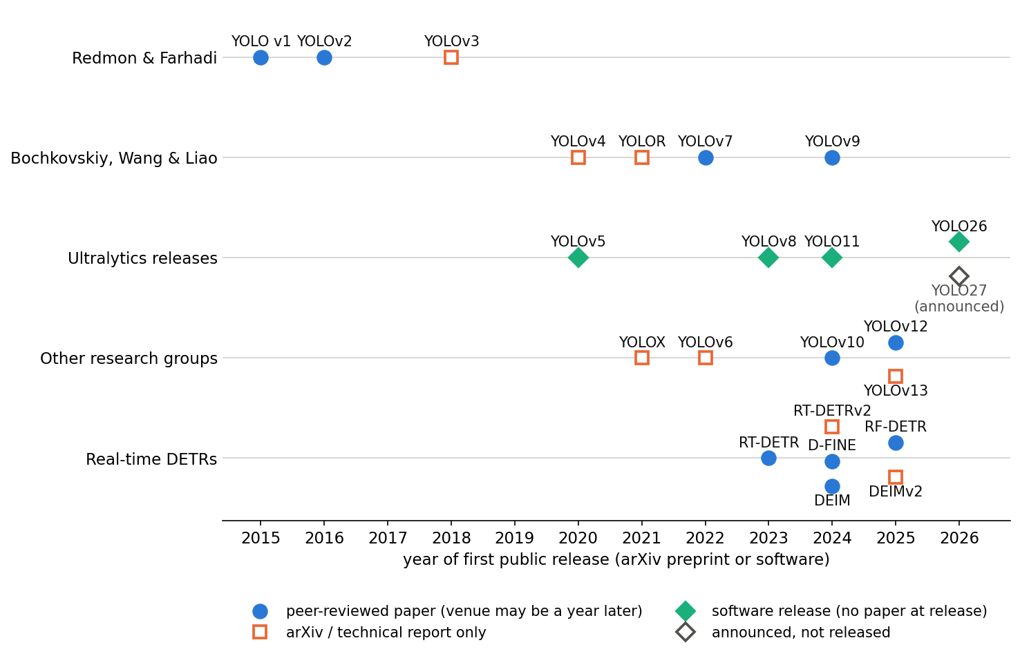
Figure 1 places the versions by the year they first appeared in public, grouped by who released them, and marks whether each has a peer-reviewed paper. Three facts are easy to miss. First, version numbers do not form one lineage: after YOLOv3, its original authors stopped, and later numbers were taken by different groups. YOLOv4 came from a new team, two of whose authors later wrote YOLOv7 and YOLOv9 [1], [2]. Second, several widely used versions (YOLOv5, YOLOv8, YOLO11) were released as software without a paper; their documentation says so [3], [4], [5]. Third, the name is unregulated: in August 2026 a preprint titled “YOLOv14” was posted to arXiv and withdrawn by its authors about two weeks later [6], so a new number by itself says nothing about quality.
The papers introduced in this chapter
The table lists every paper that has its own introduction in the Paper guides, in three groups: the one-stage detectors YOLOv4 builds on, the one-stage detectors that came after it, and the real-time DETRs, which are not one-stage detectors but now compete with them. The Ultralytics releases without a paper are summarized in the Supplementary notes.
| Paper | Year, venue | The idea in one line | Related part of YOLOv4 |
|---|---|---|---|
| Predecessors | |||
| YOLO v1 [7] | 2016, CVPR | One network regresses all boxes from an grid | Anatomy |
| YOLOv2 / YOLO9000 [8] | 2017, CVPR | k-means anchors, bounded centre offsets, multi-scale training | Head |
| YOLOv3 [9] | 2018, tech report | Three output scales, Darknet-53, logistic class scores | Head |
| SSD [10] | 2016, ECCV | Default boxes on several feature maps | Anatomy |
| RetinaNet [11] | 2017, ICCV | Focal loss for the foreground–background imbalance | Box loss |
| FCOS [12] | 2019, ICCV | Anchor-free per-pixel boxes with centre-ness | Label assignment |
| CenterNet [13] | 2019, arXiv | Objects as heatmap peaks, no IoU-based NMS | Post-processing |
| Successors | |||
| YOLOR [14] | 2021, arXiv | Learned input-independent tensors align features and refine predictions | Backbone |
| YOLOX [15] | 2021, arXiv | Anchor-free decoupled head, SimOTA assignment | Head |
| YOLOv6 [16] | 2022, tech report | Re-parameterizable backbone, task-aligned assignment, quantization | Backbone |
| YOLOv7 [1] | 2023, CVPR | E-ELAN, planned re-parameterization, lead-guided labels | Complete recipe |
| YOLOv9 [2] | 2024, ECCV | Auxiliary reversible branch for reliable gradients; GELAN | Backbone |
| YOLOv10 [17] | 2024, NeurIPS | Dual one-to-many / one-to-one heads, no NMS | Post-processing |
| YOLOv12 [18] | 2025, NeurIPS | Area attention at real-time cost | Attention |
| YOLOv13 [19] | 2025, arXiv | Hypergraph-based feature correlation | Neck |
| YOLO26 [20] | 2026, arXiv | NMS-free by default, no DFL, new optimizer and small-object assignment | Label assignment |
| Real-time DETRs | |||
| RT-DETR [21] | 2024, CVPR | Hybrid encoder, uncertainty-minimal query selection | Post-processing |
| RT-DETRv2 [22] | 2024, tech report | Per-scale sampling points, discrete sampling for deployment | Complete recipe |
| D-FINE [23] | 2025, ICLR | Boxes as distributions refined layer by layer | Box loss |
| DEIM [24] | 2025, CVPR | More positives through Mosaic-style dense one-to-one matching | Mosaic |
| RF-DETR [25] | 2026, ICLR | Weight-sharing architecture search on a DINOv2 backbone | Backbone |
| DEIMv2 [26] | 2025, arXiv | DINOv3 features adapted to multi-scale detection | Backbone |
Challenge
Plain version. YOLOv4 tests published techniques to combine accurate detection, real-time inference and training on a single conventional GPU.
A fast detector that one ordinary GPU can train
The paper (Bochkovskiy, Wang and Liao, arXiv, April 2020) [27] starts from a practical complaint: the most accurate networks of the time did not run in real time and needed many GPUs and large mini-batches to train. Its stated goal is a detector that is fast “in production systems”, meaning fast in measured frames per second on a GPU rather than small in a theoretical operation count, and that anyone can train and test on a single 1080 Ti or 2080 Ti card [27].
Two predecessors frame the problem. YOLOv3 [9] was fast but, by 2020, clearly less accurate than the best detectors on the strict COCO metric: at 608 × 608 it reached 33.0% AP in the YOLOv4 comparison table [27]. EfficientDet [28] was accurate and efficient in floating-point operations, but the paper’s measurements show that low operation counts do not translate into high GPU frame rates (see Backbone). YOLOv4 wants the accuracy of the second at the speed of the first.
What “real-time” means and how YOLOv4 times it
A detector is real-time when the time it needs per frame is shorter than the time between frames. Latency is the time from receiving one frame to having its final boxes; throughput is how many frames are finished per second when many are processed together. For one frame,
where is pre-processing (decoding, resizing and normalizing the image, copying it to the accelerator), is the forward pass of the network, and is post-processing (decoding boxes, the confidence threshold, NMS). A camera at frames per second leaves seconds per frame: about 33.3 ms at 30 FPS. With batches of frames, throughput is , where is the time for one batch; it grows with , but every frame then waits for its whole batch, so a live camera cares about latency at batch size 1. Converting latency to FPS as (with in milliseconds) is only meaningful at batch 1.
YOLOv4’s speed tables follow this convention. Their captions state that the results are compared “with batch=1 without using tensorRT”, that is, without NVIDIA’s optimizing inference engine [29], and the tables are split by GPU architecture (Maxwell, Pascal and Volta) because different papers timed their models on different cards [27]. They mark “real-time” as 30 FPS or more. The paper does not state the numeric precision or whether NMS is inside the timed interval; the YOLOX report later timed its comparisons “with FP16-precision and batch=1 on a V100 to align the settings of YOLOv4” [15]. Keep these conditions in mind when you read the numbers in Results.
Why the paper tests “freebies” and “specials”
Many published “features” claim to improve CNNs, but often only for one model, one task or small datasets. The paper therefore sorts candidate improvements into two bags and tests them [27]:
- Bag of freebies (BoF): methods that change only the training strategy or only increase the training cost, so inference stays exactly as fast. Data augmentation, regularization, label smoothing, box-regression losses and assignment rules belong here.
- Bag of specials (BoS): plug-in modules and post-processing steps that add a small inference cost but can improve accuracy noticeably. Receptive-field blocks, attention modules, feature-fusion paths, activation functions and NMS variants belong here.
The challenge, then, is not to invent one module but to find the combination that is best for a detector that must stay fast and must train on one GPU. The rest of this introduction follows the paper’s own order: the architecture it selects, the freebies and specials it adds, the experiments that justify the choices, and what remains open.
Method
Plain version. YOLOv4 retains the YOLOv3 head, adds CSPDarknet53 and an SPP/PANet neck, and combines training and inference refinements.
The detector anatomy: input, backbone, neck and head
Plain version. Almost every detector has three parts. A backbone turns the image into feature maps at several resolutions. A neck mixes information between those resolutions. A head looks at every cell of every map and predicts boxes and classes.
The paper’s Figure 2 and Section 2.1 give this vocabulary, which later papers adopted [27]:
- Input: an image, image patches or an image pyramid. YOLOv4 uses a single image resized to a square network resolution, typically 416, 512 or 608 pixels per side.
- Backbone: a network pre-trained on ImageNet [30] classification. GPU detectors use backbones such as VGG [31] or ResNet [32] variants; CPU detectors use mobile backbones.
- Neck: layers between backbone and head that collect feature maps from different stages, usually with several top-down and bottom-up paths, such as FPN [33] and PAN [34]; “additional blocks” such as SPP [35] enlarge the receptive field.
- Head: the predictor. A dense prediction head (one-stage detector) predicts at every location of the feature maps, with anchors (YOLO, SSD, RetinaNet) or without (CenterNet, FCOS). A sparse prediction head (two-stage detector, the R-CNN family) predicts only for a set of proposals.
YOLOv4’s choice, in the paper’s words reduced to a list, is: backbone CSPDarknet53 [36], neck SPP [35] and PAN [34], head YOLOv3 [9]. The head is anchor-based and one-stage: at three output strides it predicts, for each cell and each of three anchors, four box numbers, one objectness score and one score per class.
For a square input of side pixels and output strides 8, 16 and 32, the three output grids have , and cells per side, and the number of predictions per image is
where is the number of anchors per cell. At the grids are cells, so ; at they give 10,647 predictions. Each prediction is a vector of numbers for classes; with COCO’s 80 classes each output layer has channels, the value in the released configuration [37]. All of these predictions must be filtered down to a few boxes by a confidence threshold and NMS, which is why post-processing cost matters for real-time use.
Backbone: CSPDarknet53
Plain version. The backbone must see far enough to cover large objects and their context, have enough capacity for many objects at once, and run fast on a GPU. The paper compared three candidates and picked CSPDarknet53: YOLOv3’s Darknet-53 with “cross-stage partial” connections that send only half of each stage’s channels through the expensive blocks.
Why this backbone. Section 3.1 argues that a detector, unlike a classifier, needs a higher input resolution (for small objects), more layers (so the receptive field covers the larger input) and more parameters (to detect many objects of different sizes in one image). Table 1 of the paper compares three backbones at 512 × 512, with frame rates measured on an RTX 2070 [27]:
| Backbone | Receptive field | Parameters | BFLOPs | FPS (RTX 2070) |
|---|---|---|---|---|
| CSPResNeXt50 | 425 × 425 | 20.6 M | 31 | 62 |
| CSPDarknet53 | 725 × 725 | 27.6 M | 52 | 66 |
| EfficientNet-B3 [38] | 1311 × 1311 | 12.0 M | 11 | 26 |
Two lessons sit in this small table. First, operation counts do not predict GPU speed: EfficientNet-B3 needs about a fifth of CSPDarknet53’s operations but runs at less than half its frame rate. Second, the paper reports that CSPResNeXt50 is the better ImageNet classifier while CSPDarknet53 is the better COCO detector backbone, so “best classifier” and “best detector backbone” differ; the ablations in Backbones and pre-trained weights test this directly. CSPDarknet53 has 29 convolutional layers of size against 16 for CSPResNeXt50, hence its larger receptive field.
What cross-stage partial connections do. CSPNet [36] illustrates its design using DenseNet-style stages [39] and also applies it to other backbones, including ResNeXt [40]. In the DenseNet example, in which each layer receives the concatenation of all earlier outputs. The authors attribute part of the computational redundancy to duplicated gradient information. This is a design explanation, not a proof that all layers learn identical features. CSPNet splits the work. Write the base feature map of a stage as two channel groups,
where is concatenation along channels. Only goes through the stage’s blocks, producing ; their output passes through a transition layer (a convolution) to give ; then is concatenated with the untouched part and passed through a second transition layer:
where is convolution and are the transition weights. The CSPNet paper gives three purposes: splitting the paths can reduce duplicated gradient information, processing fewer channels can reduce computation, and the design can reduce memory traffic [36]. It also compares fusion orders and finds that the “fusion last” order, in which the block output is transformed before it is merged with , truncates the duplicated gradient flow and costs little accuracy [36]. Applied to Darknet-53, each residual stage becomes such a split–process–merge stage.
Activation. The backbone uses Mish (see Activation: Mish); in the released configuration, Mish appears in the backbone and the leaky rectifier in the neck and head [37].
Neck, part 1: the SPP block
Plain version. Objects can be much larger than what one cell “sees”. The SPP block lets each cell of the coarsest feature map look at a large neighbourhood cheaply, by max-pooling over windows of several sizes and stacking the results as extra channels.
Spatial pyramid pooling was introduced to turn feature maps of any size into a fixed-length vector for classification [35]. That version cannot be used inside a fully convolutional detector. YOLOv3’s SPP variant, which YOLOv4 adopts, keeps the spatial size: it applies max pooling with kernel sizes and stride 1, with padding so that the output has the same height and width, and concatenates the four results along channels [27]. For an input of shape ,
where is max pooling with stride 1 and “same” padding, and is the identity. The block is placed on the stride-32 map, where for a 608 input, so a window covers most of the map. The paper quotes YOLOv3-608 with SPP gaining 2.7% AP50 on COCO at 0.5% extra computation, and states that SPP “significantly increases the receptive field” while causing almost no reduction in speed [27]. The released configuration contains exactly the three max-pooling layers of sizes 5, 9 and 13 [37].
Code · Python · 16 lines
import numpy as np
from scipy.ndimage import maximum_filter

def spp(x, kernels=(5, 9, 13)):
    """YOLO-style SPP. x: (C, H, W). Stride-1 max pooling with 'same' padding keeps H and W;
    the input and the pooled copies are concatenated along the channel axis."""
    pooled = [maximum_filter(x, size=(1, k, k), mode="constant", cval=-np.inf) for k in kernels]
    return np.concatenate([x] + pooled, axis=0)

rng = np.random.default_rng(0)
x = rng.normal(size=(512, 19, 19))          # e.g. the stride-32 map of a 608 x 608 input
print("SPP:", x.shape, "->", spp(x).shape)

one = np.zeros((1, 19, 19)); one[0, 9, 9] = 1.0   # a single strong activation
y = spp(one)
print("cells reached by one activation per group:", [int((g > 0).sum()) for g in y])
Output
SPP: (512, 19, 19) -> (2048, 19, 19)
cells reached by one activation per group: [1, 25, 81, 169]
The channel count quadruples while the grid stays , and one strong activation now influences up to cells of the next layer. A convolution after the block reduces the channels again.
Neck, part 2: PANet path aggregation
Plain version. Deep feature maps know what is in the image; shallow ones know where edges are. A feature pyramid sends meaning downward to the fine maps; PANet adds a second path that sends precise location information back up to the coarse maps. YOLOv4 uses this two-way neck instead of YOLOv3’s one-way one, and merges the paths by concatenation instead of addition.
FPN [33] (explained in DLCV 03) builds levels by upsampling coarse features and adding them to finer ones (a top-down path). PANet [34] observed that the path from low-level features to the top of the pyramid is still very long, and added a bottom-up path augmentation. Starting from in the original paper, each new level is
where halves the resolution of , is element-wise addition with the FPN level of the same resolution, and the outer convolution produces the new map [34]. In YOLOv4 the pyramid runs over strides 8, 16 and 32, and the three outputs feed the three heads. Section 3.1 says the authors chose PANet “instead of the FPN used in YOLOv3” [27].
YOLOv4’s modification. Figure 6 of the paper replaces the shortcut (addition) in PAN with concatenation: along channels, followed by convolutions [27]. Concatenation keeps both inputs separate and lets the next convolution learn how to weight them, at the price of more channels. The paper lists this among the changes made “to make the designed detector more suitable for training on single GPU”, but it does not report a separate ablation of addition versus concatenation.
Head: the YOLOv3 head and box decoding
Plain version. At each cell, for each of three template boxes (anchors), the head outputs four numbers that move and stretch the template, one “is there an object?” score and one score per class. YOLOv4 keeps this head and fixes one numerical problem: in YOLOv3, a box centre close to a cell border was very hard to predict.
Decoding. The head follows YOLOv2 [8] and YOLOv3 [9]. For a cell whose top-left corner is at in grid units and an anchor of width and height , the network outputs and the box is
where is the logistic sigmoid, is the box centre in grid units (multiply by the stride for pixels) and its size. An objectness output gives , and each class has its own sigmoid score, so a box can carry several labels; YOLOv3 trains the class scores with binary cross-entropy [9]. Each output stride has three anchors; the released YOLOv4 configuration uses the nine anchors (in pixels) , , at stride 8, , , at stride 16 and , , at stride 32 [37].
The grid-sensitivity problem. Because never reaches 0 or 1, a centre that lies exactly on a cell border needs , and centres near borders need very large . Section 4.3 of the paper calls this “grid sensitivity”: the network must output extreme values to place a centre near or [27]. The fix is to multiply the sigmoid by a factor greater than 1. The paper states only that; the released code writes it as
where is the scale factor (scale_x_y in the configuration) and the shift keeps the range centred on the cell, so the centre can now cover , slightly beyond the cell [37]. The released configuration uses , 1.1 and 1.05 at strides 8, 16 and 32 [37]. The snippet decodes one prediction and shows how much less extreme has to be.
Code · Python · 23 lines
import numpy as np

sigmoid = lambda t: 1 / (1 + np.exp(-t))
logit = lambda p: np.log(p / (1 - p))

def decode(t, cell, anchor, stride, s=1.0):
    """One YOLOv3/YOLOv4 prediction t = (tx, ty, tw, th) -> box centre and size in pixels.
    s = 1 is the YOLOv3 formula; s > 1 is YOLOv4's grid-sensitivity fix."""
    tx, ty, tw, th = t
    bx = s * sigmoid(tx) - (s - 1) / 2 + cell[0]        # centre in grid units
    by = s * sigmoid(ty) - (s - 1) / 2 + cell[1]
    return bx * stride, by * stride, anchor[0] * np.exp(tw), anchor[1] * np.exp(th)

# cell (10, 7) of the stride-8 grid, anchor 36 x 75 pixels, raw outputs all zero
print("box (cx, cy, w, h):", np.round(decode((0, 0, 0, 0), (10, 7), (36, 75), 8), 1))

# which raw output tx puts the centre at a given position inside its cell?
for pos in (0.5, 0.9, 0.99, 1.0):
    row = []
    for s in (1.0, 1.2):
        p = (pos + (s - 1) / 2) / s                     # the sigmoid value that is needed
        row.append(f"s={s}: " + (f"{logit(p):5.2f}" if p < 1 else "  inf"))
    print(f"centre at {pos:4.2f} of the cell -> tx = " + " | ".join(row))
Output
box (cx, cy, w, h): [84. 60. 36. 75.]
centre at 0.50 of the cell -> tx = s=1.0:  0.00 | s=1.2:  0.00
centre at 0.90 of the cell -> tx = s=1.0:  2.20 | s=1.2:  1.61
centre at 0.99 of the cell -> tx = s=1.0:  4.60 | s=1.2:  2.29
centre at 1.00 of the cell -> tx = s=1.0:   inf | s=1.2:  2.40
With a centre on the border needs instead of infinity, so the targets the network must learn stay in a comfortable range. In the ablation table this is the column “S” (see Detector bag of freebies).
Training targets. The head is trained with three terms: a box loss (CIoU in YOLOv4, see Box loss), a binary cross-entropy objectness loss, and binary cross-entropy class losses on the positive predictions. In YOLOv3, a prediction whose box already overlaps a ground-truth box well but is not assigned to it is ignored in the objectness loss rather than pushed to “background”; YOLOv3 used an IoU of 0.5 for this rule [9], and the released YOLOv4 configuration sets it to 0.7 (ignore_thresh) [37]. Which predictions count as positives is the subject of the next section.
Label assignment: several anchors per object
Plain version. During training, every object must be “given” to some predictions, which are then taught to fire on it. YOLOv3 gave each object to exactly one anchor, the best-shaped one. YOLOv4 keeps this best match and can add anchors whose shapes are similar enough, so an object can train several predictions.
In YOLOv3, an object is assigned to the single anchor whose shape has the highest IoU with the object’s box, at the cell containing the object’s centre [9]. YOLOv4’s bag of freebies includes “using multiple anchors for a single ground truth”. The released code assigns the best anchor first, then adds anchors with
as positives, where the IoU compares only widths and heights (both boxes placed on the same centre) and is the “IoU threshold” hyper-parameter [27]. The genetic search (below) selected , which is also the value in the released configuration (iou_thresh) [37]. Because the nine anchors are split across three strides, one object can now be learned on two output levels. The best-anchor fallback still provides a match when no anchor passes the threshold. The snippet demonstrates shape matching; a full implementation must also handle targets competing for the same prediction.
Code · Python · 17 lines
import numpy as np

# the nine anchors (width, height in pixels) of yolov4.cfg; three per output stride
anchors = np.array([[12, 16], [19, 36], [40, 28], [36, 75], [76, 55], [72, 146],
                    [142, 110], [192, 243], [459, 401]], float)
stride = np.repeat([8, 16, 32], 3)

def shape_iou(wh, anchors):
    """IoU of boxes that share a centre: only width and height matter."""
    inter = np.minimum(wh[0], anchors[:, 0]) * np.minimum(wh[1], anchors[:, 1])
    return inter / (wh[0] * wh[1] + anchors.prod(1) - inter)

for wh in [(30, 60), (100, 90), (60, 120)]:
    iou = shape_iou(np.array(wh, float), anchors)
    pos = np.union1d([iou.argmax()], np.flatnonzero(iou > 0.213))
    print(f"object {wh[0]:3d}x{wh[1]:<3d} | best anchor {iou.argmax()} (IoU {iou.max():.2f}) | "
          f"IoU > 0.213: anchors {pos.tolist()} on strides {sorted(set(stride[pos].tolist()))}")
Output
object  30x60  | best anchor 3 (IoU 0.67) | IoU > 0.213: anchors [1, 2, 3, 4] on strides [8, 16]
object 100x90  | best anchor 6 (IoU 0.58) | IoU > 0.213: anchors [3, 4, 5, 6] on strides [16, 32]
object  60x120 | best anchor 5 (IoU 0.68) | IoU > 0.213: anchors [3, 4, 5, 6] on strides [16, 32]
Each object now trains four predictions instead of one. More positives give more training signal, especially for objects whose shape falls between two anchors, but they also teach several predictions to fire on the same object, which makes NMS indispensable. In the ablation table this is the column “IT”. Later detectors replaced fixed shape rules with assignment based on the network’s own predictions (YOLOX, YOLOv6) and eventually with one-to-one assignment that removes NMS (YOLOv10). DLCV 03 explains the IoU-based rules of two-stage detectors and of RetinaNet for comparison.
Activation: Mish
Plain version. An activation function decides how a neuron responds to its input. YOLOv3 used the leaky rectifier, which has a sharp corner at zero. Mish is a smooth curve that behaves like the identity for large inputs and lets small negative values through, which the paper found to help both the classifier and the detector.
Mish is defined as [41]
where . For large positive , and ; for large negative , it tends to 0; in between it dips slightly below zero, so it is not monotonic. The leaky rectifier of YOLO v1 to v3 is for and otherwise [7]. The paper’s activation candidates were ReLU, leaky ReLU, parametric ReLU, ReLU6, SELU, Swish [42] and Mish; it removed parametric ReLU and SELU as hard to train and ReLU6 as designed for quantized networks, and notes that Swish and Mish are both continuously differentiable [27].
Code · Python · 12 lines
import numpy as np

mish = lambda x: x * np.tanh(np.log1p(np.exp(x)))   # x * tanh(softplus(x))
leaky = lambda x: np.where(x > 0, x, 0.1 * x)         # the leaky rectifier of YOLO v1-v3

for v in (-3.0, -1.0, 0.0, 1.0, 3.0):
    print(f"x = {v:4.1f} | Mish {mish(v):7.4f} | leaky {float(leaky(v)):5.2f}")
x = np.linspace(-6, 6, 120001)
i = mish(x).argmin()
print(f"Mish minimum {mish(x[i]):.4f} at x = {x[i]:.3f}")
h = 1e-6
print(f"slope at 0: Mish {(mish(h) - mish(-h)) / (2 * h):.4f}; leaky jumps from 0.1 to 1")
Output
x = -3.0 | Mish -0.1456 | leaky -0.30
x = -1.0 | Mish -0.3034 | leaky -0.10
x =  0.0 | Mish  0.0000 | leaky  0.00
x =  1.0 | Mish  0.8651 | leaky  1.00
x =  3.0 | Mish  2.9865 | leaky  3.00
Mish minimum -0.3088 at x = -1.192
slope at 0: Mish 0.6000; leaky jumps from 0.1 to 1
Mish is smooth everywhere (its slope at 0 is 0.6, while the leaky rectifier’s slope jumps from 0.1 to 1), its smallest value is about , and for inputs above about 3 it is almost the identity. In the paper’s classifier experiments Mish raised CSPResNeXt-50’s top-1 accuracy from 77.9% to 78.9% on its own, and the detector built on the Mish-trained CSPDarknet53 was the best one (see Ablations) [27]. The price is a slightly more expensive function than a rectifier.
Box loss: from IoU to CIoU
Plain version. The box loss tells the network how wrong a predicted box is. Measuring errors in the four coordinates separately ignores that they describe one box. IoU-based losses measure the overlap instead, and the CIoU loss adds two more hints: how far apart the centres are and whether the shape is right.
The paper’s Section 2.2 retraces the history [27]. Squared error on unnormalized box coordinates depends on their units and does not directly measure overlap. UnitBox uses for overlapping boxes [43]; the commonly used overlap loss remains finite at zero overlap. The latter considers the box as a whole and is invariant to a common rescaling, but is constant with zero gradient while boxes remain disjoint. GIoU [44] adds a penalty based on the smallest box enclosing both. DIoU and CIoU [45] add a centre-distance term and, for CIoU, an aspect-ratio term. The CIoU loss for a predicted box and ground truth is
where and are the two box centres, is the Euclidean distance between them, is the diagonal length of the smallest box enclosing both, and are the widths and heights, measures the aspect-ratio mismatch and is a weight that gives the aspect term more influence once the boxes overlap well [45]. Dropping the last term gives the DIoU loss, and dropping the last two gives the IoU loss. DLCV 03 computes all four measures for disjoint and overlapping boxes; the snippet below instead splits the CIoU loss into its three parts for one tall ground-truth box.
Code · Python · 21 lines
import numpy as np

def iou_terms(a, b):
    """a, b: boxes (x1, y1, x2, y2). Returns IoU, the DIoU penalty rho^2/c^2 and the CIoU term alpha*v."""
    iw = max(0.0, min(a[2], b[2]) - max(a[0], b[0])); ih = max(0.0, min(a[3], b[3]) - max(a[1], b[1]))
    inter = iw * ih
    wa, ha, wb, hb = a[2] - a[0], a[3] - a[1], b[2] - b[0], b[3] - b[1]
    iou = inter / (wa * ha + wb * hb - inter)
    cw = max(a[2], b[2]) - min(a[0], b[0]); ch = max(a[3], b[3]) - min(a[1], b[1])
    rho2 = ((a[0] + a[2] - b[0] - b[2]) ** 2 + (a[1] + a[3] - b[1] - b[3]) ** 2) / 4
    v = 4 / np.pi ** 2 * (np.arctan(wb / hb) - np.arctan(wa / ha)) ** 2
    alpha = v / ((1 - iou) + v) if v > 0 else 0.0
    return iou, rho2 / (cw ** 2 + ch ** 2), alpha * v

gt = (100, 100, 200, 300)                                  # 100 x 200 pixels, tall
preds = {"centred, lying flat":       (50, 150, 250, 250),
         "shifted, right shape":      (125, 125, 225, 325),
         "far away":                  (300, 100, 400, 300)}
for name, p in preds.items():
    iou, d, av = iou_terms(p, gt)
    print(f"{name:26s} IoU {iou:.3f} | L_IoU {1 - iou:.3f} | L_DIoU {1 - iou + d:.3f} | L_CIoU {1 - iou + d + av:.3f}")
Output
centred, lying flat        IoU 0.333 | L_IoU 0.667 | L_DIoU 0.667 | L_CIoU 0.700
shifted, right shape       IoU 0.488 | L_IoU 0.512 | L_DIoU 0.530 | L_CIoU 0.530
far away                   IoU 0.000 | L_IoU 1.000 | L_DIoU 1.308 | L_CIoU 1.308
The centred but wrongly shaped box gets no DIoU penalty (the centres coincide) but a CIoU penalty for its shape; the shifted box of the right shape gets a distance penalty only; the far-away box has IoU 0, so the IoU loss says nothing about how far it is, while the distance term does. YOLOv4 adopts CIoU, arguing that it gives better convergence speed and accuracy [27]; the released configuration sets iou_loss=ciou with a loss weight of 0.07 (iou_normalizer, the “loss normalizer” found by the genetic search) [37].
Post-processing: NMS and DIoU-NMS
Plain version. With several positives per object, several predictions fire on each object, and non-maximum suppression keeps the best one and deletes the others that overlap it too much. Its cost depends on the scene. DIoU-NMS changes the deletion test so that two boxes whose centres are far apart are less likely to be treated as duplicates, which helps with neighbouring objects.
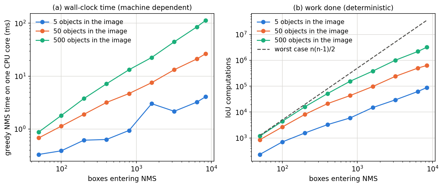
Greedy NMS and its cost. Greedy NMS (defined in DLCV 03) takes the highest-scoring box, computes its IoU with every remaining box, deletes those above a threshold, and repeats. If boxes enter and few are deleted, the number of IoU computations approaches
where counts the boxes still remaining after each kept box. If most boxes are duplicates of a few objects, they are deleted early and the work is much smaller. So NMS time depends on the number of candidates, on the confidence threshold that decides how many enter, and on the scene, unlike the forward pass, which takes about the same time for every image. The snippet times a NumPy greedy NMS on synthetic candidates; counts of IoU computations are deterministic, while the times depend on your machine.
Code · Python · 32 lines
import numpy as np

def nms_count(boxes, scores, thr=0.5):
    """Greedy NMS that also counts how many box-pair IoUs it computes."""
    order = np.argsort(-scores)
    keep, n_iou = [], 0
    while order.size:
        i, rest = order[0], order[1:]
        keep.append(i)
        n_iou += rest.size
        x1 = np.maximum(boxes[i, 0], boxes[rest, 0]); y1 = np.maximum(boxes[i, 1], boxes[rest, 1])
        x2 = np.minimum(boxes[i, 2], boxes[rest, 2]); y2 = np.minimum(boxes[i, 3], boxes[rest, 3])
        inter = np.clip(x2 - x1, 0, None) * np.clip(y2 - y1, 0, None)
        area = lambda b: (b[..., 2] - b[..., 0]) * (b[..., 3] - b[..., 1])
        iou = inter / (area(boxes[i]) + area(boxes[rest]) - inter)
        order = rest[iou <= thr]
    return len(keep), n_iou

def random_boxes(n, n_objects, rng, size=640):
    """n candidate boxes jittered around n_objects true objects."""
    centres = rng.uniform(40, size - 40, (n_objects, 2))
    owner = rng.integers(0, n_objects, n)
    c = centres[owner] + rng.normal(0, 6, (n, 2))
    wh = rng.uniform(30, 60, (n, 2))
    return np.hstack([c - wh / 2, c + wh / 2]), rng.random(n)

rng = np.random.default_rng(0)
for n_objects in (5, 500):                       # few objects vs a crowded scene
    for n in (100, 1000, 8400):
        b, s = random_boxes(n, n_objects, rng)
        kept, n_iou = nms_count(b, s)
        print(f"objects {n_objects:3d} | boxes {n:4d} | kept {kept:4d} | IoUs {n_iou:9,d}")
Output
objects   5 | boxes  100 | kept   21 | IoUs       770
objects   5 | boxes 1000 | kept   43 | IoUs     7,809
objects   5 | boxes 8400 | kept   86 | IoUs    90,699
objects 500 | boxes  100 | kept   94 | IoUs     4,621
objects 500 | boxes 1000 | kept  513 | IoUs   209,490
objects 500 | boxes 8400 | kept 1259 | IoUs 3,039,292
The printed counts are deterministic; Figure 2 separately measures wall-clock time, which varies by machine. With the same 8,400 candidates, the crowded scene needs about 34 times as many IoU computations as the sparse one. Optimized implementations can run on a GPU and cap the number of boxes, so these counts are a toy analysis rather than a runtime prediction: post-processing time grows with the number of candidates and with crowding. Figure 2 repeats the experiment over a range of candidate counts. This is the cost that the NMS-free successors remove (YOLOv10, RT-DETR); the RT-DETR paper measured it directly for real detectors.
DIoU-NMS. Greedy NMS deletes a box when its IoU with the kept box exceeds the threshold, so two real people standing close together can be merged into one. The DIoU paper proposed to subtract the centre-distance penalty before the test [45]:
where is the score of (0 means deleted), is the distance between the centres and , is the diagonal of the box enclosing both, and is the NMS threshold. Two boxes with distant centres “probably locate different objects” and survive more easily [45]. YOLOv4 lists DIoU-NMS in its bag of specials for the detector [27]. The snippet repeats the box geometry so it can be run on its own.
Code · Python · 27 lines
import numpy as np

def iou_terms(a, b):
    """a, b: boxes (x1, y1, x2, y2). Returns IoU, the DIoU penalty rho^2/c^2 and the CIoU term alpha*v."""
    iw = max(0.0, min(a[2], b[2]) - max(a[0], b[0])); ih = max(0.0, min(a[3], b[3]) - max(a[1], b[1]))
    inter = iw * ih
    wa, ha, wb, hb = a[2] - a[0], a[3] - a[1], b[2] - b[0], b[3] - b[1]
    iou = inter / (wa * ha + wb * hb - inter)
    cw = max(a[2], b[2]) - min(a[0], b[0]); ch = max(a[3], b[3]) - min(a[1], b[1])
    rho2 = ((a[0] + a[2] - b[0] - b[2]) ** 2 + (a[1] + a[3] - b[1] - b[3]) ** 2) / 4
    v = 4 / np.pi ** 2 * (np.arctan(wb / hb) - np.arctan(wa / ha)) ** 2
    alpha = v / ((1 - iou) + v) if v > 0 else 0.0
    return iou, rho2 / (cw ** 2 + ch ** 2), alpha * v


def nms(boxes, scores, thr=0.5, diou=False):
    order, keep = list(np.argsort(-scores)), []
    while order:
        m = order.pop(0); keep.append(int(m))
        crit = lambda j: iou_terms(boxes[m], boxes[j])[0] - (iou_terms(boxes[m], boxes[j])[1] if diou else 0)
        order = [j for j in order if crit(j) < thr]
    return keep

# two people side by side (centres 32 px apart) and one duplicate of the first person
boxes = np.array([[100, 100, 200, 200], [132, 100, 232, 200], [103, 100, 203, 200]], float)
scores = np.array([0.9, 0.8, 0.7])
print("greedy NMS keeps:", nms(boxes, scores), "| DIoU-NMS keeps:", nms(boxes, scores, diou=True))
Output
greedy NMS keeps: [0] | DIoU-NMS keeps: [0, 1]The second person overlaps the first with IoU 0.515, just above the threshold, so greedy NMS deletes it; the distance penalty lowers the criterion to 0.478 and DIoU-NMS keeps it, while the near-duplicate (centres 3 pixels apart) is still removed. The effect is confined to a narrow band of overlaps, and cannot resolve all crowded-scene ambiguity. The YOLOv4 ablations do not isolate its contribution.
Data augmentation: Mosaic and CutMix
Plain version. Mosaic glues four training images into one, so every training image shows objects in four different contexts and at smaller sizes. It is the augmentation most associated with YOLOv4 and the one most copied by later detectors.
Section 2.2 of the paper surveys pixel-wise augmentations (photometric changes, random scaling, cropping, flipping, rotation), occlusion-style augmentations that erase rectangles, and augmentations that combine images: MixUp [46] blends two images with weights and and blends their labels the same way, and CutMix [47] pastes a rectangle from one image into another and mixes the labels in proportion to the pasted area [27]. YOLOv4 uses CutMix for the backbone’s classifier training and introduces Mosaic, which “mixes 4 training images” [27]. The paper’s acknowledgements credit Glenn Jocher for the idea of Mosaic, along with the genetic hyper-parameter search and the grid-sensitivity fix [27].
The paper gives two reasons for Mosaic: objects are seen “outside their normal context”, and batch normalization computes its statistics from four different images per training image, which “significantly reduces the need for a large mini-batch size” [27]. That second reason links Mosaic to the single-GPU goal.
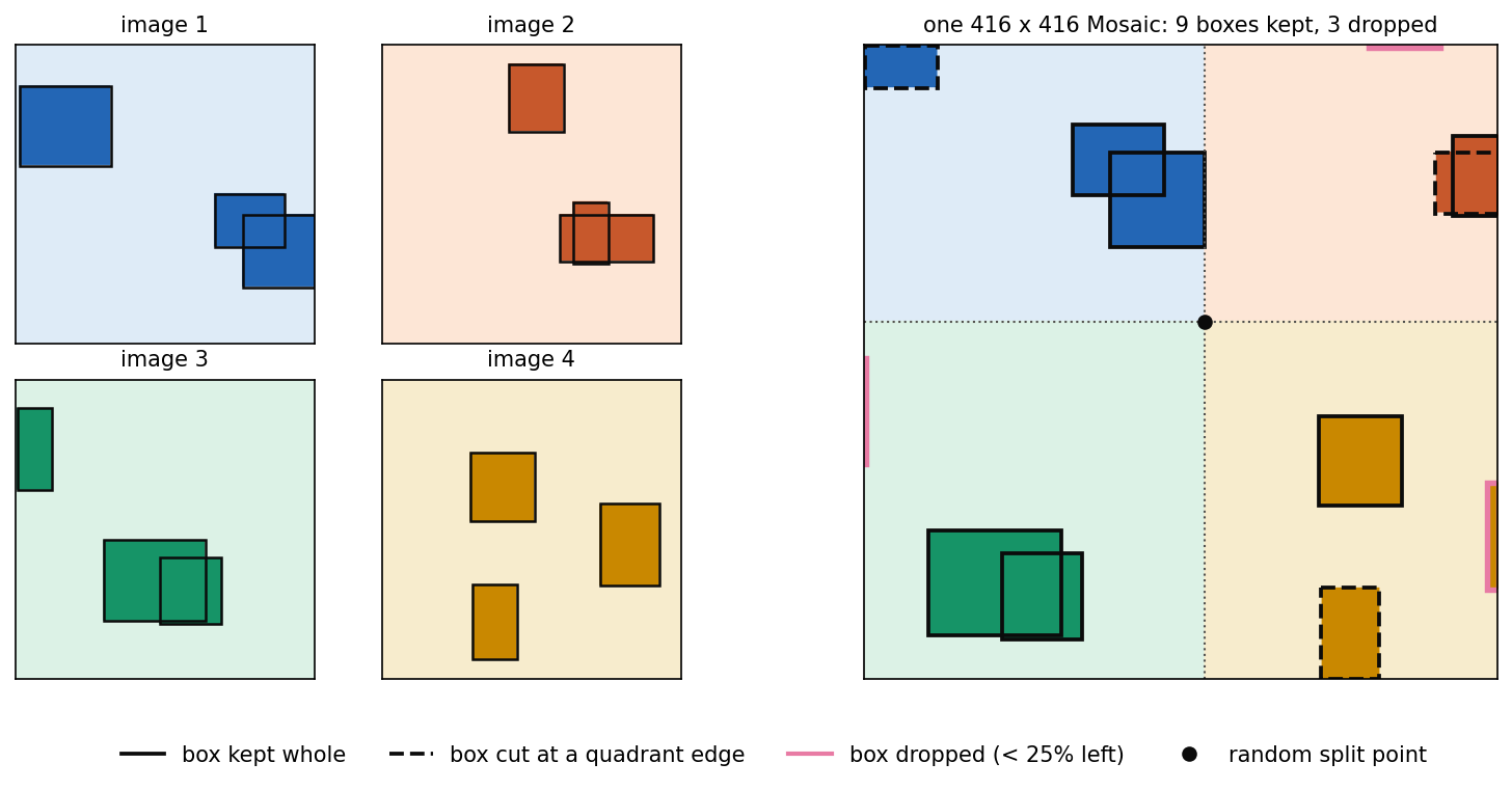
The paper does not specify the procedure in more detail than its Figure 3, and implementations differ in how they scale and crop. A simple version, written out below, chooses a random split point on the output canvas, places the four images so that each touches the split point with one corner, cuts away whatever falls outside each image’s quadrant, and clips or drops the boxes accordingly.
Code · Python · 40 lines
import numpy as np

def mosaic(images, boxes, size=416, rng=None, min_keep=0.25):
    """Place four images around a random split point (xc, yc) of a size x size canvas.
    images: four (H, W, 3) arrays; boxes: four (n, 4) arrays of (x1, y1, x2, y2) in pixels.
    Each image touches the split point with one corner; whatever falls outside its quadrant is cut.
    A box is kept if at least `min_keep` of its area survives the cut."""
    xc, yc = (int(v) for v in rng.uniform(0.3, 0.7, 2) * size)
    canvas = np.full((size, size, 3), 114, np.uint8)
    out, n_cut, n_drop = [], 0, 0
    for k, (img, bx) in enumerate(zip(images, boxes)):
        h, w = img.shape[:2]
        ox = xc - w if k in (0, 2) else xc          # where the image's top-left corner lands
        oy = yc - h if k in (0, 1) else yc
        rx0, rx1 = (0, xc) if k in (0, 2) else (xc, size)   # the quadrant it may fill
        ry0, ry1 = (0, yc) if k in (0, 1) else (yc, size)
        x0, x1, y0, y1 = max(rx0, ox), min(rx1, ox + w), max(ry0, oy), min(ry1, oy + h)
        canvas[y0:y1, x0:x1] = img[y0 - oy:y1 - oy, x0 - ox:x1 - ox]
        shifted = bx + [ox, oy, ox, oy]
        clipped = np.clip(shifted, [x0, y0, x0, y0], [x1, y1, x1, y1])
        area = lambda b: (b[:, 2] - b[:, 0]) * (b[:, 3] - b[:, 1])
        keep = area(clipped) >= min_keep * area(shifted)
        n_cut += int((keep & (area(clipped) < area(shifted))).sum()); n_drop += int((~keep).sum())
        out.append(clipped[keep])
    return canvas, np.concatenate(out), (xc, yc), n_cut, n_drop

rng = np.random.default_rng(0)
imgs, bxs = [], []
for k in range(4):                                   # four synthetic 256 x 256 "photos"
    img = np.full((256, 256, 3), 60 * k + 40, np.uint8)
    b = []
    for _ in range(3):                               # three rectangles = three objects each
        x, y = rng.integers(0, 200, 2); w, h = rng.integers(30, 90, 2)
        x2, y2 = min(x + w, 256), min(y + h, 256)
        img[y:y2, x:x2] = rng.integers(0, 256, 3); b.append([x, y, x2, y2])
    imgs.append(img); bxs.append(np.array(b, float))

canvas, boxes, split, n_cut, n_drop = mosaic(imgs, bxs, rng=rng)
print("canvas", canvas.shape, "| split point", split)
print(f"objects in: {sum(len(b) for b in bxs)} | kept: {len(boxes)} (of which cut: {n_cut}) | dropped: {n_drop}")
Output
canvas (416, 416, 3) | split point (223, 181)
objects in: 12 | kept: 9 (of which cut: 3) | dropped: 3
Figure 3 draws this example. Three of the twelve objects survive only partly and three are cut away almost completely; the rule for dropping a box (here, less than a quarter of its area left) is an implementation choice that the paper does not discuss. Mosaic later became the standard YOLO augmentation, and DEIM uses it for a different purpose: to put more objects in each image so that one-to-one matching receives more positives.
Self-adversarial training
Plain version. Self-adversarial training (SAT) first lets the network change the training image, not its weights, so that the image fools the network into seeing no object; then it trains the network on that altered image in the normal way. It is a data augmentation generated by the detector itself.
The paper introduces SAT as “a new data augmentation technique that operates in 2 forward backward stages” [27]. In the first stage the network “alters the original image instead of the network weights”, executing “an adversarial attack on itself” to create “the deception that there is no desired object”; in the second stage it is “trained to detect an object on this modified image in the normal way” [27]. The paper describes the stages in words only. One way to write them, in our notation rather than the paper’s, is
where is the training image, its boxes and labels, the detector with weights , the detection loss, the size of the image change (the weights are frozen during this step) and the learning rate. Stage 1 moves the image to increase the chosen objective; increasing a generic detection loss can also disturb localization rather than merely hide an object. This illustrative objective is not an exact SAT specification from the paper; stage 2 is an ordinary training step on the altered image. SAT requires additional training computation and adds no inference stage; the paper does not separately measure its training-time overhead. The paper lists SAT among the detector’s bag of freebies, but its ablation tables contain no SAT column, so its contribution is not measured separately (see Limits of the evidence).
Regularization: DropBlock and class label smoothing
Plain version. Regularizers make training harder on purpose so that the network does not memorize the training set. DropBlock switches off whole square patches of a feature map instead of scattered single units; label smoothing tells the network never to be completely sure about a class.
DropBlock. Dropout [48] zeroes random units independently. In a convolutional feature map, neighbouring units are strongly correlated, so a zeroed unit can be reconstructed from its neighbours and dropout regularizes weakly. DropBlock [49] zeroes contiguous blocks. Following its Algorithm 1: sample seed positions only where a whole block fits inside the map, zero a square around each seed, multiply the activations by the mask, and rescale them by to compensate approximately for the fraction of surviving activations [49]. To drop roughly a fraction of the units on a map, the seed probability is
where is the keep probability as in dropout, the block size, the feature-map size and the number of valid seed positions; the formula is approximate because blocks can overlap [49]. The DropBlock paper also found that a fixed hurts early training and gradually decreases it from 1 to the target value [49].
Code · Python · 21 lines
import numpy as np

def dropblock_mask(feat, block, keep_prob, rng):
    """One DropBlock mask for a feat x feat map (Ghiasi et al., Algorithm 1)."""
    gamma = (1 - keep_prob) / block ** 2 * feat ** 2 / (feat - block + 1) ** 2
    half = block // 2
    seeds = np.zeros((feat, feat), bool)                       # only where a whole block fits
    seeds[half:feat - half, half:feat - half] = rng.random((feat - block + 1,) * 2) < gamma
    mask = np.ones((feat, feat))
    for i, j in zip(*np.nonzero(seeds)):
        mask[i - half:i + half + 1, j - half:j + half + 1] = 0.0
    return mask, gamma

rng = np.random.default_rng(0)
feat, block, keep = 38, 7, 0.9
masks = [dropblock_mask(feat, block, keep, rng)[0] for _ in range(2000)]
gamma = dropblock_mask(feat, block, keep, rng)[1]
dropped = 1 - np.mean([m.mean() for m in masks])
print(f"gamma = {gamma:.5f} | target drop rate {1 - keep:.2f} | measured {dropped:.3f}")
m = masks[0]
print("first mask: dropped units", int((m == 0).sum()), "| rescale factor", round(m.size / m.sum(), 3))
Output
gamma = 0.00288 | target drop rate 0.10 | measured 0.094
first mask: dropped units 171 | rescale factor 1.134
On a map with blocks, a seed probability below 0.3% already removes about 9.4% of the units, a little less than the 10% target because overlapping blocks are counted once. YOLOv4 chose DropBlock “without hesitation” because its authors’ comparison with other methods was favourable [27], and lists it in both the backbone’s and the detector’s bag of freebies; the detector ablation table has no DropBlock column.
Class label smoothing. With hard one-hot targets, cross-entropy keeps pushing the correct logit up, which encourages over-confidence. Label smoothing [50] replaces the target distribution by
where indexes the classes, is the true class, is 1 if and 0 otherwise, and is the smoothing amount [50]. YOLOv4’s detector uses independent sigmoid scores, and its ablation table describes LS as “class label smoothing for sigmoid activation” [27]; for one two-way sigmoid output the same formula with moves the targets from 1 and 0 to and . The paper does not state the value of . Label smoothing helped the classifier (CSPResNeXt-50: 77.9% → 78.1% top-1) but lowered the detector’s AP when used alone (38.0% → 33.0%; see Detector bag of freebies) [27].
Normalization: cross mini-batch normalization
Plain version. Batch normalization needs statistics computed over many images. On one GPU, a detector only fits a few images at a time. Cross mini-batch normalization (CmBN) collects the statistics over the several small mini-batches that together make up one training batch.
Batch normalization [51] normalizes each channel with the mean and variance of the current mini-batch : , where is an activation, are learned scale and shift and is a small constant. With only 4 or 8 images per mini-batch these statistics are noisy. Cross-iteration batch normalization (CBN) [52] averages statistics over several recent training iterations; because the weights change between iterations, it compensates the old statistics with a Taylor-polynomial approximation of how they would look under the current weights [52]. Synchronizing statistics across GPUs does not solve the single-GPU constraint.
YOLOv4 trains with a batch of 64 images split into mini-batches of 8 or 4 (the configuration’s subdivisions), and the weights are updated once per batch [27], [37]. CmBN “collects statistics only between mini-batches within a single batch” [27]. In our reading of the paper’s Figure 4, the statistics used for the -th mini-batch of a batch accumulate those of mini-batches of the same batch, for example
where is the -th equally sized mini-batch and the variances are population moments. Averaging variances alone would omit differences between mini-batch means. Since weights do not change inside this batch, no cross-update compensation is needed. This illustrates correct moment aggregation; it is not an equation supplied by YOLOv4 or a complete specification of its released implementation. In the ablation (column CBN) CmBN alone gave 38.4% AP against the baseline’s 38.0% [27].
Attention and fusion: the modified SAM and weighted residuals
Plain version. An attention module lets the network re-weight its features, emphasizing informative positions. YOLOv4 takes the spatial attention module of CBAM and simplifies it to an element-wise gate. It also lists a learned-weight way of adding feature maps, taken from EfficientDet.
SAM. The spatial attention module of CBAM [53] pools the feature map along the channel axis by average and by max, concatenates the two maps, and convolves them:
where is a convolution, the sigmoid and multiplication broadcast over channels, so one weight per position scales all channels [53]. The paper notes that SAM costs about 0.1% extra computation on ImageNet classifiers and “does not affect the speed of inference on the GPU at all”, whereas it estimates that the representative channel-attention module adds about 10% to GPU inference time [27]. YOLOv4 modifies SAM “from spatial-wise attention to point-wise attention” (its Figure 5): in that figure the two pooling steps are replaced by a convolution applied to itself, so the gate has the same shape as and scales every element separately [27]. In the specials ablation, adding SAM to CSPResNeXt50-PANet-SPP raised AP from 42.4% to 42.7% [27].
Multi-input weighted residual connections (MiWRC). EfficientDet’s feature network adds several inputs with learned non-negative weights, using “fast normalized fusion” [28]:
where are the input feature maps, (enforced by a ReLU) are learned weights and avoids division by zero [28]. YOLOv4 lists MiWRC in the bag of specials for the backbone but reports no experiment that isolates it.
Training schedule: cosine annealing, genetic search and random shapes
Plain version. Several freebies concern how training is run rather than what the network computes: how the learning rate changes, how the many hyper-parameters are chosen, and which input sizes the network sees.
Cosine annealing. Instead of dropping the learning rate in steps, SGDR [54] lowers it along half a cosine:
where and bound the learning rate, counts the epochs since the last restart and is the length of the current cycle, so falls smoothly from to [54]. YOLOv4’s column CA (“altering the learning rate during sinusoid training”) gave 38.7% AP alone against 38.0% for the step schedule [27].
Genetic hyper-parameter search (GA). A genetic algorithm keeps a population of hyper-parameter settings, trains briefly with each, keeps the best (the “fittest”), and creates new settings by mutating and combining them. The paper uses it “for selecting the optimal hyperparameters during network training on the first 10% of time periods” [27]. The search ran YOLOv3-SPP with the GIoU loss for 300 epochs on a 5,000-image “min-val” set and selected a learning rate of 0.00261, momentum 0.949, the assignment IoU threshold 0.213 and the box-loss normalizer 0.07 [27]. Alone, GA gave 38.9% AP against 38.0% [27].
Random training shapes and dynamic mini-batch size. Like YOLOv2’s multi-scale training [8], YOLOv4 changes the input resolution during training (“random training shapes”) so that one model works at several resolutions [27]. “Dynamic mini-batch size” (DM) automatically increases the mini-batch size when the random shape is small, so that the GPU is used fully; alone it lowered AP to 35.3% [27].
Optimized anchors (OA). The anchors are re-estimated for the 512 × 512 training resolution, in the spirit of YOLOv2’s k-means “dimension clusters” (explained in the DLCV 03 Supplementary notes) [27].
The complete recipe
Plain version. Putting the pieces together, YOLOv4 is CSPDarknet53 + SPP + PAN + YOLOv3 head, trained with a long list of freebies and fitted with a few cheap specials.
Section 3.4 of the paper lists the final model as follows [27]:
| Part | What YOLOv4 uses | Kind |
|---|---|---|
| Backbone | CSPDarknet53 | architecture |
| Neck | SPP, PAN (modified: concatenation) | architecture |
| Head | YOLOv3 (anchor-based, 3 scales × 3 anchors) | architecture |
| Backbone, freebies | CutMix and Mosaic, DropBlock, class label smoothing | training only |
| Backbone, specials | Mish, cross-stage partial connections, MiWRC | small inference cost |
| Detector, freebies | CIoU loss, CmBN, DropBlock, Mosaic, self-adversarial training, grid-sensitivity elimination, multiple anchors per ground truth, cosine annealing, genetically searched hyper-parameters, random training shapes | training only |
| Detector, specials | Mish, SPP block, modified SAM, modified PAN, DIoU-NMS | small inference cost |
Later detectors kept the overall shape of this recipe (a CSP-style backbone, an FPN–PAN neck, Mosaic, IoU-based losses, many positives per object) and replaced specific items; Problems maps those changes to the components above.
Results
Plain version. On COCO, YOLOv4 reached 43.5% AP at 608 × 608. Its 416-pixel model exceeded 30 FPS on all three tested GPU generations; the 608-pixel model reached only 23 FPS on Maxwell. The useful result is a measured speed–accuracy trade-off, not real-time operation for every resolution and GPU.
Training and evaluation setup
All detector experiments train on COCO [55] and report accuracy on test-dev 2017 with the COCO AP metrics [56] (AP averaged over IoU thresholds 0.50 to 0.95, plus AP50, AP75 and AP for small, medium and large objects) [27]. The classifier experiments train on ImageNet [30] and report ILSVRC 2012 validation accuracy [27].
The detector’s default schedule is 500,500 training steps with a step-decay learning rate starting at 0.01 and multiplied by 0.1 at steps 400,000 and 450,000; momentum 0.9 and weight decay 0.0005; one GPU, multi-scale training, a batch size of 64 and a mini-batch size of 8 or 4 depending on memory [27]. The classifier’s default is 8,000,000 steps, batch 128 with mini-batch 32, a polynomial-decay learning rate starting at 0.1 with 1,000 warm-up steps, momentum 0.9 and weight decay 0.005; the BoF classifier experiments train 50% longer [27]. Everything runs on a single 1080 Ti or 2080 Ti [27].
The main comparison
Tables 8, 9 and 10 of the paper compare YOLOv4 with other detectors on COCO test-dev, one table per GPU architecture: Maxwell (GTX Titan X or Tesla M40), Pascal (Titan X Pascal, Titan Xp, GTX 1080 Ti or Tesla P100) and Volta (Titan Volta or Tesla V100), all “with batch=1 without using tensorRT” [27]. YOLOv4’s own rows are identical in accuracy across the three tables, because only the speed is re-measured:
| Input | AP | AP50 | AP75 | APS | APM | APL | FPS Maxwell | FPS Pascal | FPS Volta |
|---|---|---|---|---|---|---|---|---|---|
| 416 | 41.2 | 62.8 | 44.3 | 20.4 | 44.4 | 56.0 | 38 | 54 | 96 |
| 512 | 43.0 | 64.9 | 46.5 | 24.3 | 46.1 | 55.2 | 31 | 43 | 83 |
| 608 | 43.5 | 65.7 | 47.3 | 26.7 | 46.7 | 53.3 | 23 | 33 | 62 |
How to read it against the other rows:
- Against YOLOv3 (Table 8, Maxwell): YOLOv3-608 reaches 33.0% AP and YOLOv3-SPP-608 36.2% AP, both at 20 FPS, so YOLOv4-608 is about 10 AP points more accurate at a slightly higher frame rate on the same GPU class [27].
- Against EfficientDet (Table 10, Volta): EfficientDet-D0 to D3 reach 33.8%, 39.6%, 43.0% and 45.8% AP at 62.5, 50.0, 41.7 and 23.8 FPS. YOLOv4-512 matches D2’s 43.0% AP at 83 FPS instead of 41.7; D3 is more accurate (45.8%) but runs at 23.8 FPS, below the 30 FPS line [27]. This is the basis of the paper’s claim that YOLOv4 runs about twice as fast as EfficientDet at comparable accuracy.
- Against the slower, more accurate detectors: several two-stage and keypoint-based detectors in Table 9 reach higher AP (the highest, 46.8%, runs at 1.3 FPS), but none of them is real-time [27]. YOLOv4 does not claim the highest AP overall, only the best accuracy among detectors at 30 FPS or more.
Two details deserve attention. First, the large-object AP falls as the input grows (56.0 → 55.2 → 53.3), while small-object AP rises from 20.4 to 26.7; a larger input helps small objects but makes large objects relatively larger than the receptive field and the anchors were tuned for. Second, the abstract quotes “∼65 FPS on Tesla V100” for the 43.5% AP model, while Table 10 lists 62 FPS for it [27]; the table is the more specific source.
Speed: a measurement checklist
When you measure, or read, a latency number for any detector, check the following; each item is a condition YOLOv4’s tables fix, leave open, or vary.
- Hardware, engine and precision are stated and the same for every model being compared. YOLOv4 states the GPU family and “without TensorRT”, but not the precision.
- Batch size 1 for latency; throughput numbers with large batches do not transfer to a live camera.
- End to end: pre-processing, the network and post-processing including NMS, or a clear statement of what is excluded. YOLOv4 does not state whether NMS is timed; its successors’ end-to-end benchmarks add NMS explicitly (see RT-DETR and YOLOv10), averaged over the COCO validation images because NMS time depends on the image.
- Same device, not only the same architecture family: YOLOv4’s tables group cards of one GPU generation (for example a Titan X Maxwell and a Tesla M40), and the speeds of other methods come from their own papers, so small FPS differences between rows are not measurements on identical hardware.
- Warm-up and averaging: the first iterations of any engine are slow (memory allocation, kernel selection), so discard them and average over many images.
- Input size and confidence threshold used during timing; for NMS-based detectors, the threshold used for computing AP (often very low) also changes the post-processing time.
Ablations
Plain version. The paper’s experiments are a long series of “try one change, keep it if it helps” tables: first for the backbone as a classifier, then for the detector’s freebies and specials, then for the backbone choice and the mini-batch size. Reading them carefully shows which components really matter and which were kept on weaker evidence.
Classifier ablations
Tables 2 and 3 train the two candidate backbones as ImageNet classifiers with different freebies and activations (top-1 / top-5 accuracy) [27].
| CSPResNeXt-50 setting | Top-1 | Top-5 |
|---|---|---|
| baseline | 77.9 | 94.0 |
| MixUp | 77.2 | 94.0 |
| CutMix | 78.0 | 94.3 |
| Mosaic | 78.1 | 94.5 |
| bilateral blurring | 77.5 | 93.8 |
| label smoothing | 78.1 | 94.4 |
| Swish | 64.5 | 86.0 |
| Mish | 78.9 | 94.5 |
| CutMix + Mosaic + label smoothing | 78.5 | 94.8 |
| CutMix + Mosaic + label smoothing + Mish | 79.8 | 95.2 |
For CSPDarknet-53 the baseline is 77.2 / 93.6, the three freebies give 77.8 / 94.4 and adding Mish gives 78.7 / 94.8 [27]. What this proves: CutMix, Mosaic, label smoothing and Mish each help the classifier, and they combine; MixUp and blurring do not. The Swish row (64.5%) stands out; the paper does not discuss it, and a drop that large looks more like a failed training run than a property of the activation, so it should not be read as evidence against Swish in general.
Detector bag of freebies
Table 4 tests detector freebies on CSPResNeXt50-PANet-SPP at 512 × 512 [27]. The columns are S (grid-sensitivity elimination), M (Mosaic), IT (several anchors per ground truth above the IoU threshold), GA (genetic hyper-parameters), LS (class label smoothing), CBN (CmBN), CA (cosine annealing), DM (dynamic mini-batch size), OA (optimized anchors) and the box loss. Reading the rows in groups:
| Rows | Setting | AP | AP50 | AP75 |
|---|---|---|---|---|
| baseline | MSE loss, no freebie | 38.0 | 60.0 | 40.8 |
| one freebie, MSE loss | S | 37.7 | 59.9 | 40.5 |
| M | 39.1 | 61.8 | 42.0 | |
| IT | 36.9 | 59.7 | 39.4 | |
| GA | 38.9 | 61.7 | 41.9 | |
| LS | 33.0 | 55.4 | 35.4 | |
| CBN | 38.4 | 60.7 | 41.3 | |
| CA | 38.7 | 60.7 | 41.9 | |
| DM | 35.3 | 57.2 | 38.0 | |
| S + loss | GIoU / DIoU / CIoU | 39.4 / 39.1 / 39.6 | 59.4 / 58.8 / 59.2 | 42.5 / 42.1 / 42.6 |
| combinations | S + M + IT + GA, CIoU | 41.5 | 64.0 | 44.8 |
| M + GA + OA, CIoU | 36.1 | 56.5 | 38.4 | |
| S + M + IT + GA + OA, MSE | 40.3 | 64.0 | 43.1 | |
| S + M + IT + GA + OA, GIoU | 42.4 | 64.4 | 45.9 | |
| S + M + IT + GA + OA, CIoU | 42.4 | 64.4 | 45.9 |
What the table proves:
- Mosaic is the strongest single freebie (+1.1 AP alone), followed by GA, cosine annealing and CmBN, which each add a few tenths.
- IoU-type losses beat MSE, and among them CIoU is best by a small margin when combined with S (39.6 against 39.4 for GIoU); in the best combination GIoU and CIoU tie at 42.4.
- Some freebies hurt in isolation: S alone (−0.3), IT alone (−1.1), DM (−2.7) and LS (−5.0). S and IT pay off only in combination: S + M + IT + GA with CIoU reaches 41.5, and the best setting, 42.4 AP, includes both. A plausible reading is that more positives (IT) and wider centre ranges (S) need the stronger training of the combined recipe; the paper does not analyse it.
- The best rows do not contain LS, CBN, CA or DM, although Section 3.4 lists label smoothing, CmBN and cosine annealing in YOLOv4’s detector freebies. The table never shows a row with all of the final freebies together, so their joint effect on the detector is not measured here.
Detector bag of specials
Table 5 adds modules to CSPResNeXt50-PANet-SPP at 512 × 512 [27]: the base with SPP and PAN reaches 42.4% AP; adding SAM gives 42.7% (AP50 64.6, AP75 46.3); the other combinations it tests (a receptive-field block, a Gaussian box-uncertainty head on top of SAM, and an adaptive feature-fusion block with the receptive-field block) all lower AP, to between 41.1% and 41.8% [27]. What it proves: SPP, PAN and SAM are the useful specials for this detector; adding more modules is not free. DIoU-NMS, Mish in the detector and MiWRC have no row.
Backbones and pre-trained weights
Table 6 trains the detector with different classifier weights for initialization, all at 512 × 512 with otherwise similar settings [27]:
| Detector backbone (initialized from) | AP | AP50 | AP75 |
|---|---|---|---|
| CSPResNeXt50 (default classifier) | 42.4 | 64.4 | 45.9 |
| CSPResNeXt50 (classifier with BoF) | 42.3 | 64.3 | 45.7 |
| CSPResNeXt50 (classifier with BoF + Mish) | 42.3 | 64.2 | 45.8 |
| CSPDarknet53 (classifier with BoF) | 42.4 | 64.5 | 46.0 |
| CSPDarknet53 (classifier with BoF + Mish) | 43.0 | 64.9 | 46.5 |
What it proves: for CSPResNeXt50, a better classifier (79.8% instead of 77.9% top-1) does not give a better detector; for CSPDarknet53, the better classifier does. This is the experimental basis for the backbone choice, and the general lesson that ImageNet accuracy is a poor proxy for detection quality.
Mini-batch size
Table 7 trains with mini-batches of 4 and 8 images [27]. Without the freebies and specials, CSPResNeXt50-PANet-SPP at 608 reaches 37.1% AP with mini-batch 4 and 38.4% with mini-batch 8; with them, CSPDarknet53-PANet-SPP at 512 reaches 41.6% and 41.7%. What it proves, within this setting: after the full recipe the mini-batch size “has almost no effect”, which supports the claim that the detector can be trained well on one conventional GPU. Mosaic’s four-images-per-sample statistics and CmBN are the components designed for this; the table does not separate their contributions.
Conclusion
YOLOv4 shows that a classic one-stage, anchor-based detector, given a stronger backbone and neck and a carefully tested set of training tricks, can match much slower detectors in accuracy while running in real time, and can be trained on a single consumer GPU. Its experiments establish that Mosaic, IoU-type box losses, genetic hyper-parameter search, more positives per object, SPP, PAN and point-wise SAM help such a detector, that some popular tricks do not, and that the best classifier backbone is not automatically the best detector backbone. The paper’s lasting contribution is less any single module than the vocabulary (backbone, neck, head; freebies and specials) and the practice of testing training tricks on the detector itself.
Problems
Plain version. YOLOv4 kept the parts that later detectors found most limiting: anchors, a shared head for classes and boxes, many positives per object and therefore NMS. Its evidence also has gaps: several listed components are never tested on the detector, the ablations are single runs on the test set, and the paper was never peer reviewed.
Limits of the method
- Anchors are dataset-specific. The nine anchors are clustered for COCO (and re-optimized for one input size); a new dataset or resolution needs new anchors, and an object whose shape matches no anchor is learned poorly. YOLOX argues exactly this when it drops anchors.
- A coupled head. One set of convolutions predicts classes and boxes together. YOLOX shows that separating them speeds up convergence.
- Fixed-rule assignment. Positives are chosen by anchor shape and object centre, not by how well the network currently predicts; later work assigns positives from the network’s own predictions (SimOTA in YOLOX, task-aligned assignment in YOLOv6).
- NMS dependency. Several positives per object make NMS necessary, with its threshold to tune, its cost that grows with the scene (Figure 2) and its failure on neighbouring objects; DIoU-NMS only narrows that failure. The NMS-free line starts with YOLOv10.
- Large objects at high resolution. APL drops from 56.0 at 416 to 53.3 at 608 in the paper’s own results [27].
Limits of the evidence
- Not peer reviewed. YOLOv4 exists as an arXiv preprint [27]; it was never published at a reviewed venue (unlike YOLOv7, by two of the same authors).
- Ablations on test-dev, single runs. The detector ablations report test-dev results, a split intended for final evaluation, and give single numbers without variance; differences of a few tenths of AP may be within run-to-run variation.
- Untested components. Self-adversarial training, DropBlock in the detector, DIoU-NMS, MiWRC and the PAN modification have no ablation row, and no row combines all the final freebies. The final recipe therefore includes components whose effect on this detector is asserted rather than measured.
- Speed conditions. Numeric precision and the treatment of NMS are not stated, and competitor speeds come from other papers on the same GPU generation, not the same card. The abstract’s “∼65 FPS” and Table 10’s 62 FPS disagree slightly.
The paper and the released configuration
The configuration file cfg/yolov4.cfg in the authors’ repository (as accessed for this chapter) differs from the paper’s list in places [37]: it uses a step learning-rate schedule (policy=steps, steps 400,000 and 450,000) rather than cosine annealing, greedy NMS (nms_kind=greedynms) rather than DIoU-NMS, and contains no SAM or DropBlock layer, while it does use Mosaic, the CIoU loss, the grid-sensitivity factors and the 0.213 assignment threshold. Its learning rate is 0.0013 rather than the 0.00261 found by the genetic search. A repository file can change after publication, so this does not show what was used for the paper’s tables; it shows that “YOLOv4” in practice may not include every item of Section 3.4, which matters when you compare reproductions.
Export, reduced precision and re-parameterization
Training frameworks are not deployment engines. A trained detector is usually exported to an exchange format such as ONNX [57] and compiled by an inference engine for the target device, for example TensorRT for NVIDIA GPUs [29]. Three things change on the way:
- Precision. FP16 uses half the storage per represented value compared with FP32; the speed and accuracy changes depend on the graph and runtime. INT8 quantization represents selected weights and activations with 8-bit integers and scale parameters [58]. Calibration or quantization-aware training is needed. Validate all output stages and check AP at strict IoU thresholds after quantizing, not only AP50. YOLOv6 reports that re-parameterized models are harder to quantize and changes its training to fix this [16].
- Graph simplification. Batch normalization is folded into the preceding convolution, and re-parameterized multi-branch blocks (used from YOLOv6 and YOLOv7 on) are folded into single convolutions; the folding is derived in the Supplementary notes.
- Unsupported operators and post-processing. Every operator must exist in the target engine. Mish, for example, is a less common operator than a rectifier. RT-DETRv2 adds a discrete sampling operator for this reason [22], and YOLO26 cites simpler export as one reason for removing its distribution-based box head [20]. Removing NMS can simplify one part of export, but decoding, score selection and coordinate restoration still have to be implemented and timed.
Optional: Folding a re-parameterized block into one convolution (in the Supplementary notes). The batch-norm folding formula and a NumPy check that three branches become one convolution with the same output.
What later one-stage detectors changed
Each change below replaces or extends one YOLOv4 component; the linked paper guides explain the method in full.
| YOLOv4 component | What came later | Paper |
|---|---|---|
| Anchor-based coupled head | Anchor-free decoupled head, one prediction per location | YOLOX |
| Fixed-rule positives (IoU of shapes > 0.213) | Prediction-aware assignment: SimOTA, then task-aligned assignment | YOLOX, YOLOv6 |
| CSPDarknet53 blocks | Re-parameterizable blocks folded into plain convolutions for inference | YOLOv6, YOLOv7 |
| Training only the final head | Auxiliary heads and branches that supervise the network during training only | YOLOv7, YOLOv9 |
| Several positives + NMS (DIoU-NMS) | A one-to-one head trained alongside a one-to-many head; no NMS | YOLOv10, YOLO26 |
| SAM, a cheap spatial gate | Real self-attention made affordable (area attention); hypergraph correlation | YOLOv12, YOLOv13 |
| CIoU on four box numbers | Distribution-based box sides (DFL), later removed again | YOLOv6, YOLO26 |
| SGD with step or cosine schedule | MuSGD, a hybrid of SGD and the Muon optimizer | YOLO26 |
What stayed: the CSP idea in backbones, an FPN-plus-PAN neck, Mosaic, IoU-type box losses and the habit of measuring speed on real hardware.
Beyond one-stage: real-time DETRs
Plain version. DETR showed that a transformer can output the final set of boxes directly, with one prediction per object and no NMS, but it was slow to train and slow to run. Real-time DETRs keep the direct-set idea and redesign the expensive parts; they are not one-stage dense detectors, but since 2023 they compete with YOLOs at the same speed.
DETR [59] and its descendants are introduced in DLCV 03. The real-time line that started with RT-DETR differs from YOLOv4 in exactly the component that YOLOv4 left untouched: it trains with one-to-one (Hungarian [60]) matching, so each object has a single prediction and no NMS is needed. Each paper has its own introduction in the Paper guides:
| Paper | What it changes |
|---|---|
| RT-DETR | A hybrid encoder (attention on the coarsest level only, convolutional fusion across levels), uncertainty-minimal query selection, adjustable decoder depth, and an end-to-end speed benchmark that times NMS for YOLOs |
| RT-DETRv2 | Per-scale sampling points, an optional discrete sampling operator for deployment, dynamic augmentation and scale-specific learning rates |
| D-FINE | Box edges as probability distributions refined decoder layer by layer, with self-distillation from the last layer |
| DEIM | More positives under one-to-one matching through Mosaic and MixUp, and a matchability-aware classification loss |
| RF-DETR | A DINOv2 backbone and weight-sharing architecture search that yields many speed–accuracy trade-offs without retraining |
| DEIMv2 | DINOv3 features turned into multi-scale features by a light adapter, plus pruned convolutional backbones for the smallest models |
Modern view
What the surveys say
A Comprehensive Review of YOLO Architectures in Computer Vision: From YOLOv1 to YOLOv8 and YOLO-NAS (Terven, Córdova-Esparza and Romero-González, Machine Learning and Knowledge Extraction, 2023) [61] walks through 16 versions in order, starting from the metrics and post-processing, then the architecture and training tricks of each. Its discussion organizes the history by four axes: anchors (absent in YOLO v1, added in YOLOv2, removed again from YOLOX on), framework (Darknet, then PyTorch), backbone (Darknet, then cross-stage partial connections, re-parameterization and architecture search), and the constant speed–accuracy trade-off. It expects COCO to be replaced by harder benchmarks and YOLO models to expand into tracking and multimodal tasks.
YOLO Evolution: A Comprehensive Benchmark and Architectural Review of YOLOv12, YOLO11, and Their Previous Versions (Jegham, Koh, Abdelatti and Hendawi, arXiv, 2024, revised 2025) [62] is an experimental comparison rather than a history: it evaluates versions from YOLOv3 to YOLOv12 on datasets chosen for varying object sizes, aspect ratios and small single-class objects, and reports precision, recall, mAP, processing time, GFLOPs and model size. Its takeaway is that no version wins everywhere: in its experiments YOLO11 gave the best overall balance, YOLOv10 was fast but weaker on overlapping objects, and YOLOv12’s added complexity did not pay off. Treat these as one group’s results on its datasets, not general rankings.
Ultralytics YOLO Evolution: An Overview of YOLO27, YOLO26, YOLO11, YOLOv8, and YOLOv5 (Sapkota and Karkee, arXiv, 2025, revised 2026) [63] reviews only the Ultralytics releases, covering architecture, benchmarking, deployment (export and quantization) and applications, and lists open challenges: dense scenes, combining CNNs with transformers, open-vocabulary perception, domain generalization and hardware-aware optimization. It is a third-party review, not an Ultralytics publication.
Object Detection with Transformers: A Review (Shehzadi et al., Sensors, 2025) [64] covers the DETR side: improvements to DETR grouped by backbone, query design and attention mechanism, which is the context for the real-time DETRs.
The state of the art, 2023–2026
- NMS-free is becoming the default. YOLOv10 [17] introduced it to YOLOs in 2024; YOLO26 [20] ships it as the default deployment path; the real-time DETRs discussed here omit NMS at inference. The announced YOLO27 describes query-based decoding without NMS for its larger models [65].
- Attention is affordable. YOLOv12 [18] and YOLOv13 [19] put attention-like modules inside YOLOs, where YOLOv4 could only afford a cheap spatial gate; RT-DETR [21] restricts attention to the coarsest level.
- Pretrained vision transformers as backbones. RF-DETR [25] and DEIMv2 [26] start from self-supervised backbones (DINOv2 [66], DINOv3 [67]), whose benefits must be checked separately for accuracy, transfer and latency.
- Training efficiency. DEIM [24] and YOLO26 (with a new optimizer and a progressive loss) target shorter training rather than only higher AP, a direct descendant of YOLOv4’s single-GPU goal.
Open problems
- Fair speed comparison. There is no shared, maintained end-to-end benchmark across devices; most tables still mix conditions, and RF-DETR shows that even GPU power throttling changes reported latencies.
- Small and crowded objects remain the main accuracy gap at real-time input sizes; YOLO26’s small-object assignment and DEIMv2’s unchanged small-object AP both illustrate it.
- Quantization-friendly heads. Score and box outputs lose accuracy at INT8, and attention layers complicate low-precision deployment.
- Peer review and reproducibility. YOLOv4 itself and several widely deployed successors have no peer-reviewed paper, released code can differ from the paper, and version numbers are claimed freely; claims need independent checks.
- Beyond closed sets. Bringing open-vocabulary detection to the same latency as closed-set YOLOs without losing accuracy.
Key takeaways
- Real-time performance is an end-to-end latency budget on a stated device, not an isolated FPS value.
- YOLOv4 combines CSPDarknet53, SPP and a modified PANet with the YOLOv3 head.
- Distinguish training-only techniques from inference components when interpreting cost.
- Ablations support some components more directly than others; isolated gains and combined gains can differ.
- Classifier accuracy and operation counts do not determine detector accuracy or measured speed.
- Later detectors revisit heads, assignment, matching and feature fusion; compare complete training and inference settings.
Exercises
- Budget arithmetic. A camera runs at 25 FPS. Pre-processing takes 3 ms, the network 18 ms, and NMS between 1 ms (empty street) and 9 ms (crowd). Does the system keep up in both cases, and how much time is left for tracking? Which single change would help most in crowds?
Hint
The budget is 40 ms. The total is 22 ms in the empty street and 30 ms in the crowd, leaving 18 ms and 10 ms. The NMS term is the only one that depends on the scene, so an NMS-free head (or a higher confidence threshold, at a cost in recall) helps most in crowds.
- Count YOLOv4’s predictions. How many predictions does YOLOv4 make for a 512 × 512 input, and how many for a 1024 × 1024 input? If NMS cost grew with the square of the number of candidates entering it, how much more expensive would NMS be at 1024 than at 512 when the same fraction of candidates survives the confidence threshold?
Hint
At 512 the grids are cells, times 3 anchors = 16,128 predictions. At 1024 the count is four times larger, 64,512. A fourfold increase in candidates gives a sixteenfold increase in the worst-case number of IoU computations; real NMS sits between linear and quadratic growth, as the snippet’s crowded and sparse scenes show.
- Grid sensitivity by hand. With (YOLOv4’s stride-16 setting), which range of centre offsets inside a cell can the head produce, and which places the centre exactly on the cell’s right border? Modify the decoding snippet to check your answer.
Hint
The offset ranges over . The right border (offset 1) needs , so .
- DropBlock budget. On a map with block size 7, what seed probability targets a drop rate of 10%? Use the snippet to measure the actual drop rate and explain why it differs more from 10% than on the map.
Hint
. On a small map, a larger share of seeds produce blocks that overlap each other, and only seed positions are valid, so overlap and the approximation in the formula matter more; expect a measured rate noticeably below 10%.
- Design a better ablation. Table 4 tests most freebies one at a time against a weak baseline and in a few combinations. Design an experiment that measures the contribution of each of YOLOv4’s final detector freebies in the presence of all the others. How many training runs does it need, and what would you report besides the mean AP?
Hint
A leave-one-out ablation: train the full recipe once, then once without each component (about a dozen runs for the detector’s freebies), with several seeds per setting so that you can report a standard deviation. Evaluate on a validation split (val2017), not test-dev, and report AP, AP50, AP75 and the size-specific APs, plus training time, since some freebies (self-adversarial training) cost training time.
- Two speed tables. Paper A reports 4.1 ms on an A100 GPU, FP16, batch 32, forward pass only. Paper B reports 6.3 ms on a T4 GPU, FP16, batch 1, end to end with NMS. List every reason why you cannot conclude that A is faster, and design the experiment that would let you compare them.
Hint
Different GPUs, different batch sizes (A’s per-image time at batch 32 hides latency), different timed stages (A excludes pre- and post-processing). Run both exported models on one device with one engine and precision, at batch 1, at the same input size, timing end to end over the same images after warm-up, with the confidence threshold you will deploy.
Detections from a real-time detector are the input to tracking, covered in DLCV 07 · Object Tracking.
References
- C.-Y. Wang, A. Bochkovskiy and H.-Y. M. Liao, “YOLOv7: Trainable bag-of-freebies sets new state-of-the-art for real-time object detectors,” in Proc. IEEE/CVF CVPR, pp. 7464–7475, 2023. doi
- C.-Y. Wang, I-H. Yeh and H.-Y. M. Liao, “YOLOv9: Learning what you want to learn using programmable gradient information,” in Proc. ECCV, 2024. doi
- G. Jocher, “Ultralytics YOLOv5,” software (first released 2020; v7.0 released 22 November 2022). release · documentation
- G. Jocher, A. Chaurasia and J. Qiu, “Ultralytics YOLOv8,” software, version 8.0.0, 2023 (no paper). docs · code
- G. Jocher and J. Qiu, “Ultralytics YOLO11,” software, version 11.0.0, 2024 (no paper). docs · code
- J. Lu, J. Jia, J. Yawl and C. Zhang, “YOLOv14: Adaptive real-time object detection for diverse imaging conditions,” arXiv:2608.04720, 2026 (withdrawn by the authors, 20 August 2026). arXiv
- J. Redmon, S. Divvala, R. Girshick and A. Farhadi, “You only look once: Unified, real-time object detection,” in Proc. IEEE CVPR, pp. 779–788, 2016. doi · arXiv
- J. Redmon and A. Farhadi, “YOLO9000: Better, faster, stronger,” in Proc. IEEE CVPR, pp. 6517–6525, 2017. doi · arXiv
- J. Redmon and A. Farhadi, “YOLOv3: An incremental improvement,” tech. report, arXiv:1804.02767, 2018. arXiv
- W. Liu, D. Anguelov, D. Erhan, C. Szegedy, S. Reed, C. Fu, A. C. Berg, “SSD: Single Shot MultiBox Detector,” Lecture Notes in Computer Science / Computer Vision – ECCV 2016, 2016. doi · manuscript
- T.-Y. Lin, P. Goyal, R. Girshick, K. He and P. Dollár, “Focal loss for dense object detection,” in Proc. IEEE ICCV, pp. 2999–3007, 2017. doi
- Z. Tian, C. Shen, H. Chen, T. He, “FCOS: Fully Convolutional One-Stage Object Detection,” 2019 IEEE/CVF International Conference on Computer Vision (ICCV), 2019. doi · manuscript
- X. Zhou, D. Wang, P. Krähenbühl, “Objects as Points,” arXiv preprint, 2019. source
- C. Wang, I. Yeh, H. M. Liao, “You Only Learn One Representation: Unified Network for Multiple Tasks,” arXiv preprint, 2021. source
- Z. Ge, S. Liu, F. Wang, Z. Li and J. Sun, “YOLOX: Exceeding YOLO series in 2021,” arXiv:2107.08430, 2021. arXiv
- C. Li, L. Li, H. Jiang, K. Weng, Y. Geng et al., “YOLOv6: A single-stage object detection framework for industrial applications,” tech. report, arXiv:2209.02976, 2022. arXiv
- A. Wang, H. Chen, L. Liu, K. Chen, Z. Lin, J. Han and G. Ding, “YOLOv10: Real-time end-to-end object detection,” in Proc. NeurIPS, 2024. arXiv
- Y. Tian, Q. Ye and D. Doermann, “YOLOv12: Attention-centric real-time object detectors,” in Advances in Neural Information Processing Systems 38 (NeurIPS), 2025. proceedings · arXiv
- M. Lei, S. Li, Y. Wu, H. Hu, Y. Zhou et al., “YOLOv13: Real-time object detection with hypergraph-enhanced adaptive visual perception,” arXiv:2506.17733, 2025. arXiv
- G. Jocher, J. Qiu, M. Liu, S. Lyu, F. C. Akyon and M. E. Kalfaoglu, “Ultralytics YOLO26: Unified real-time end-to-end vision models,” arXiv:2606.03748, 2026 (software released January 2026). arXiv · docs
- Y. Zhao, W. Lv, S. Xu, J. Wei, G. Wang, Q. Dang, Y. Liu, J. Chen, “DETRs Beat YOLOs on Real-time Object Detection,” Proceedings of the IEEE/CVF Conference on Computer Vision and Pattern Recognition, 2024. source
- W. Lv, Y. Zhao, Q. Chang, K. Huang, G. Wang and Y. Liu, “RT-DETRv2: Improved baseline with bag-of-freebies for real-time detection transformer,” arXiv:2407.17140, 2024. arXiv
- Y. Peng, H. Li, P. Wu, Y. Zhang, X. Sun and F. Wu, “D-FINE: Redefine regression task in DETRs as fine-grained distribution refinement,” in Proc. ICLR, 2025. arXiv · code
- S. Huang, Z. Lu, X. Cun, Y. Yu, X. Zhou, X. Shen, “DEIM: DETR with Improved Matching for Fast Convergence,” Proceedings of the IEEE/CVF Conference on Computer Vision and Pattern Recognition, 2025. source
- I. Robinson, P. Robicheaux, M. Popov, D. Ramanan and N. Peri, “RF-DETR: Neural architecture search for real-time detection transformers,” in Proc. ICLR, 2026. arXiv
- S. Huang, Y. Hou, L. Liu, X. Yu and X. Shen, “Real-time object detection meets DINOv3,” arXiv:2509.20787, 2025 (revised 2026). arXiv
- A. Bochkovskiy, C.-Y. Wang and H.-Y. M. Liao, “YOLOv4: Optimal speed and accuracy of object detection,” arXiv:2004.10934, 2020. arXiv
- M. Tan, R. Pang, Q. V. Le, “EfficientDet: Scalable and Efficient Object Detection,” 2020 IEEE/CVF Conference on Computer Vision and Pattern Recognition (CVPR), 2020. doi · manuscript
- NVIDIA, “TensorRT documentation,” official documentation. link
- J. Deng, W. Dong, R. Socher, L. Li, Kai Li, Li Fei-Fei, “ImageNet: A large-scale hierarchical image database,” 2009 IEEE Conference on Computer Vision and Pattern Recognition, 2009. source
- K. Simonyan, A. Zisserman, “Very Deep Convolutional Networks for Large-Scale Image Recognition,” arXiv preprint, 2014. source
- K. He, X. Zhang, S. Ren, J. Sun, “Deep Residual Learning for Image Recognition,” arXiv preprint, 2015. source
- T.-Y. Lin, P. Dollár, R. Girshick, K. He, B. Hariharan and S. Belongie, “Feature pyramid networks for object detection,” in Proc. IEEE CVPR, 2017. doi
- S. Liu, L. Qi, H. Qin, J. Shi and J. Jia, “Path aggregation network for instance segmentation,” in Proc. IEEE/CVF CVPR, pp. 8759–8768, 2018. doi
- K. He, X. Zhang, S. Ren, J. Sun, “Spatial Pyramid Pooling in Deep Convolutional Networks for Visual Recognition,” Lecture Notes in Computer Science / Computer Vision – ECCV 2014, 2014. doi · manuscript
- C.-Y. Wang, H.-Y. M. Liao, I-H. Yeh, Y.-H. Wu, P.-Y. Chen and J.-W. Hsieh, “CSPNet: A new backbone that can enhance learning capability of CNN,” CVPR Workshops, 2020. arXiv · doi
- A. Bochkovskiy and contributors, “Darknet: YOLOv4 configuration and detection layer,” official implementation, accessed 2 November 2026. configuration · assignment and decoding
- M. Tan, Q. V. Le, “EfficientNet: Rethinking Model Scaling for Convolutional Neural Networks,” ICML, 2019. source · proceedings
- G. Huang, Z. Liu, L. Van Der Maaten, K. Q. Weinberger, “Densely Connected Convolutional Networks,” 2017 IEEE Conference on Computer Vision and Pattern Recognition (CVPR), 2017. doi · manuscript
- S. Xie, R. Girshick, P. Dollar, Z. Tu, K. He, “Aggregated Residual Transformations for Deep Neural Networks,” 2017 IEEE Conference on Computer Vision and Pattern Recognition (CVPR), 2017. doi · manuscript
- D. Misra, “Mish: A Self Regularized Non-Monotonic Activation Function,” BMVC, 2020. source
- P. Ramachandran, B. Zoph, Q. V. Le, “Searching for Activation Functions,” arXiv preprint, 2017. source
- J. Yu, Y. Jiang, Z. Wang, Z. Cao, T. Huang, “UnitBox: An Advanced Object Detection Network,” ACM Multimedia, 2016. source
- H. Rezatofighi, N. Tsoi, J. Gwak, A. Sadeghian, I. Reid, S. Savarese, “Generalized Intersection over Union: A Metric and A Loss for Bounding Box Regression,” arXiv preprint, 2019. source
- Z. Zheng, P. Wang, W. Liu, J. Li, R. Ye and D. Ren, “Distance-IoU loss: Faster and better learning for bounding box regression,” in Proc. AAAI, pp. 12993–13000, 2020. doi
- H. Zhang, M. Cisse, Y. N. Dauphin and D. Lopez-Paz, “mixup: Beyond empirical risk minimization,” in Proc. ICLR, 2018. arXiv
- S. Yun, D. Han, S. Chun, S. J. Oh, Y. Yoo, J. Choe, “CutMix: Regularization Strategy to Train Strong Classifiers With Localizable Features,” 2019 IEEE/CVF International Conference on Computer Vision (ICCV), 2019. doi · manuscript
- Nitish Srivastava, Geoffrey Hinton, Alex Krizhevsky, Ilya Sutskever, Ruslan Salakhutdinov, “Dropout: A Simple Way to Prevent Neural Networks from Overfitting,” Journal of Machine Learning Research, 2014. source
- G. Ghiasi, T. Lin, Q. V. Le, “DropBlock: A regularization method for convolutional networks,” NeurIPS, 2018. source · proceedings
- C. Szegedy, V. Vanhoucke, S. Ioffe, J. Shlens, Z. Wojna, “Rethinking the Inception Architecture for Computer Vision,” 2016 IEEE Conference on Computer Vision and Pattern Recognition (CVPR), 2016. doi · manuscript
- S. Ioffe and C. Szegedy, “Batch normalization: Accelerating deep network training by reducing internal covariate shift,” in Proc. ICML, PMLR vol. 37, pp. 448–456, 2015. link
- Z. Yao, Y. Cao, S. Zheng, G. Huang, S. Lin, “Cross-Iteration Batch Normalization,” 2021 IEEE/CVF Conference on Computer Vision and Pattern Recognition (CVPR), 2021. doi · manuscript
- S. Woo, J. Park, J. Lee, I. S. Kweon, “CBAM: Convolutional Block Attention Module,” Lecture Notes in Computer Science / Computer Vision – ECCV 2018, 2018. doi · manuscript
- I. Loshchilov, F. Hutter, “SGDR: Stochastic Gradient Descent with Warm Restarts,” ICLR, 2017. source
- T.-Y. Lin, M. Maire, S. Belongie, J. Hays, P. Perona, D. Ramanan, P. Dollár and C. L. Zitnick, “Microsoft COCO: Common objects in context,” in Proc. ECCV, pp. 740–755, 2014. doi
- COCO Consortium, “COCO detection evaluation,” official evaluation description. link
- ONNX, “Open Neural Network Exchange,” official project page. link
- B. Jacob, S. Kligys, B. Chen, M. Zhu, M. Tang, A. Howard, H. Adam and D. Kalenichenko, “Quantization and training of neural networks for efficient integer-arithmetic-only inference,” in Proc. IEEE/CVF CVPR, pp. 2704–2713, 2018. doi
- N. Carion, F. Massa, G. Synnaeve, N. Usunier, A. Kirillov and S. Zagoruyko, “End-to-end object detection with transformers,” in Proc. ECCV, 2020. doi
- H. W. Kuhn, “The Hungarian method for the assignment problem,” Naval Research Logistics Quarterly, vol. 2, pp. 83–97, 1955. doi
- J. Terven, D.-M. Córdova-Esparza and J.-A. Romero-González, “A comprehensive review of YOLO architectures in computer vision: From YOLOv1 to YOLOv8 and YOLO-NAS,” Machine Learning and Knowledge Extraction, vol. 5, no. 4, pp. 1680–1716, 2023. doi · arXiv
- N. Jegham, C. Y. Koh, M. Abdelatti and A. Hendawi, “YOLO evolution: A comprehensive benchmark and architectural review of YOLOv12, YOLO11, and their previous versions,” arXiv:2411.00201, 2024 (revised 2025). arXiv
- R. Sapkota and M. Karkee, “Ultralytics YOLO evolution: An overview of YOLO27, YOLO26, YOLO11, YOLOv8, and YOLOv5 object detectors for computer vision and pattern recognition,” arXiv:2510.09653, 2025 (revised 2026). arXiv
- T. Shehzadi, K. A. Hashmi, M. Liwicki, D. Stricker and M. Z. Afzal, “Object detection with transformers: A review,” Sensors, vol. 25, no. 19, 2025. doi
- Ultralytics, “YOLO27 (coming soon),” official documentation page, accessed 2 November 2026. docs
- M. Oquab, T. Darcet, T. Moutakanni, H. Vo, M. Szafraniec et al., “DINOv2: Learning robust visual features without supervision,” arXiv:2304.07193, 2023. arXiv
- O. Siméoni, H. V. Vo, M. Seitzer, F. Baldassarre, M. Oquab et al., “DINOv3,” arXiv:2508.10104, 2025. arXiv
- X. Ding, X. Zhang, N. Ma, J. Han, G. Ding and J. Sun, “RepVGG: Making VGG-style ConvNets great again,” in Proc. IEEE/CVF CVPR, pp. 13728–13737, 2021. doi
- R. Girshick, “Fast R-CNN,” 2015 IEEE International Conference on Computer Vision (ICCV), 2015. doi · manuscript
- S. Ren, K. He, R. Girshick, J. Sun, “Faster R-CNN: Towards Real-Time Object Detection with Region Proposal Networks,” arXiv preprint, 2015. source
- M. Everingham, L. Van Gool, C. K. I. Williams, J. Winn, A. Zisserman, “The Pascal Visual Object Classes (VOC) Challenge,” International Journal of Computer Vision, 2009. source
- A. Shrivastava, A. Gupta, R. Girshick, “Training Region-Based Object Detectors with Online Hard Example Mining,” 2016 IEEE Conference on Computer Vision and Pattern Recognition (CVPR), 2016. doi · manuscript
- H. Zhang, Y. Wang, F. Dayoub and N. Sünderhauf, “VarifocalNet: An IoU-aware dense object detector,” in Proc. IEEE/CVF CVPR, pp. 8510–8519, 2021. doi
- YOLOX contributors, “YOLOX detection head,” official implementation, accessed 2 November 2026. code
- K. Duan, S. Bai, L. Xie, H. Qi, Q. Huang, Q. Tian, “CenterNet: Keypoint Triplets for Object Detection,” arXiv preprint, 2019. source
- Z. Ge, S. Liu, Z. Li, O. Yoshie and J. Sun, “OTA: Optimal transport assignment for object detection,” in Proc. IEEE/CVF CVPR, pp. 303–312, 2021. doi
- C. Li, L. Li, Y. Geng, et al., “YOLOv6 v3.0: A Full-Scale Reloading,” arXiv preprint, 2023. source
- C. Feng, Y. Zhong, Y. Gao, M. R. Scott, W. Huang, “TOOD: Task-Aligned One-Stage Object Detection,” Proceedings of the IEEE/CVF International Conference on Computer Vision, 2021. source
- Z. Gevorgyan, “SIoU Loss: More Powerful Learning for Bounding Box Regression,” arXiv preprint, 2022. source
- X. Li, W. Wang, L. Wu, S. Chen, X. Hu, J. Li, J. Tang and J. Yang, “Generalized focal loss: Learning qualified and distributed bounding boxes for dense object detection,” in Advances in Neural Information Processing Systems 33 (NeurIPS), 2020. proceedings
- X. Ding, H. Chen, X. Zhang, K. Huang, J. Han, G. Ding, “Re-parameterizing Your Optimizers rather than Architectures,” ICLR, 2023. source
- S. Zhang, C. Chi, Y. Yao, Z. Lei, S. Z. Li, “Bridging the Gap Between Anchor-Based and Anchor-Free Detection via Adaptive Training Sample Selection,” 2020 IEEE/CVF Conference on Computer Vision and Pattern Recognition (CVPR), 2020. doi · manuscript
- C. Wang, H. M. Liao, I. Yeh, “Designing Network Design Strategies Through Gradient Path Analysis,” arXiv preprint, 2022. source
- T. Dao, D. Fu, S. Ermon, A. Rudra, C. Ré, “FlashAttention: Fast and Memory-Efficient Exact Attention with IO-Awareness,” Advances in Neural Information Processing Systems 35, 2022. doi · manuscript
- D. P. Kingma, J. Ba, “Adam: A Method for Stochastic Optimization,” ICLR, 2015. source
- K. Jordan, “Muon: An optimizer for hidden layers in neural networks,” technical blog, 2024. source
- S. Shao, Z. Li, T. Zhang, C. Peng, G. Yu, X. Zhang, J. Li, J. Sun, “Objects365: A Large-Scale, High-Quality Dataset for Object Detection,” Proceedings of the IEEE/CVF International Conference on Computer Vision, 2019. source
Check your understanding
This tutorial has 6 exercises. Can you solve them without opening the hints?
Go to the exercises ↑Next DLCV 03B · 3D Object Detection: LiDAR, Cameras and Bird's-Eye View · 42 min