DLCV 09A · Non-Blind Image Super-Resolution
Needs: DLCV 09 · Deep Image Restoration: Low-Level Vision, IP 02 · Digital Image Fundamentals, IP 04 · Filtering in the Frequency Domain
Navigate: this page and this track: Navigate: this page and this track
On this page
- What you’ll learn1 min
- The big picture2 min
- The problem: one input, many answers6 min
- The benchmark setting: a known degradation2 min
- Classical baselines5 min
- Deep SR networks: a story of design decisions12 min
- Perceptual and adversarial SR3 min
- Diffusion SR for a known degradation2 min
- When the degradation is unknown: blind and real-world SR1 min
- Arbitrary-scale SR1 min
- Efficiency1 min
- Evaluating SR3 min
- Datasets and benchmarks1 min
- Failure modes1 min
- Modern view2 min
- Key takeaways1 min
- Exercises5 min
- Supplementary notes
- References
Deep Learning for Computer Vision
Explore this chapter 2 interactive experiments
A blurry observation fits two sharp clean signals. The blurry average has the lowest expected squared error; a sharp guess looks better but is usually farther from the truth.
What you’ll learn
- Explain why super-resolution is ambiguous even with known degradation.
- Distinguish MSE’s conditional mean from L1’s coordinate-wise median.
- Compare upsampling, residual learning, normalization and attention choices.
- Interpret the fidelity–realism tradeoff of perceptual and generative objectives.
- Evaluate with explicit color, border and degradation protocols, and inspect artifacts.
The big picture
Super-resolution makes a small image bigger and sharper. Stretching the pixels is easy; the hard part is filling in detail that the small image never recorded. A modern SR network fills it in from what it learned about natural images, and that is both its strength and its risk.
Why it matters: phones zoom digitally, games and video are rendered small and upscaled, and satellites and microscopes are limited by their optics. SR is also where many low-level vision ideas were first tested, from residual learning to diffusion priors.
Scope. This chapter is about non-blind single-image SR: the way the low-resolution image was made is known and fixed, usually bicubic downscaling. The network designs were developed and compared in this setting, so it is the clearest place to learn them. Blind and real-world SR, where the degradation is unknown, is in DLCV 09A.1; video SR in DLCV 09A.3; GAN and diffusion priors for restoration in general in DLCV 09B; the generic losses and metrics in DLCV 09. You should know basic interpolation (IP 02) and aliasing (IP 04).
The running example. Most code and figures use one case: the astronaut image from skimage.data (512 × 512), shrunk by 4 with a known blur and block averaging, then enlarged back. All code uses NumPy, SciPy, scikit-image, scikit-learn and OpenCV and runs on a CPU in seconds.
The problem: one input, many answers
Question. What exactly is lost when an image is shrunk, and what does a network trained to minimize pixel error do about it? Short answer: many high-resolution images shrink to the same small image, and squared error targets their mean, which can blur disagreeing edges and textures.
Setup and notation
Single-image super-resolution (SISR) estimates a high-resolution (HR) image from one low-resolution (LR) image , where is the scale factor (2, 3, 4, …), the LR size and the number of color channels. The standard forward model, introduced in DLCV 09, is
where is a blur kernel (the camera’s optics and pixel integration, or a deliberate anti-aliasing filter), is 2-D convolution applied to each channel, keeps one sample out of every block, and is noise. In non-blind SR, , and the noise level are known at inference. They can vary if the method accepts them as conditions. This chapter mainly studies fixed benchmark degradations, where the training and test operators match; a separate network is often trained for each . Combining several shifted LR images of the same scene, the older multi-frame form of the problem [1], is the subject of DLCV 09A.3.
Why the problem is ill-posed
Count the numbers. Each LR pixel summarizes HR pixels, so the HR image has times more unknowns than there are measurements. At , there are 16 HR values per LR measurement in the overall dimension count. Even a full-row-rank, noise-free linear degradation therefore leaves at least 15 unconstrained HR dimensions per measurement. Blur can mix neighbouring blocks, so these are degrees of freedom of the whole operator, not 15 independently invisible pixels in each block. In linear-algebra terms, the degradation operator has a large null space: any HR pattern with can be added to a solution without changing . Fine textures, the exact position of an edge and small text live largely in that null space.
So SR needs a prior , a model of which HR images are plausible. With Bayes’ rule, every HR candidate gets a posterior probability
where is the likelihood (how well explains given the noise) and the prior. Classical methods write the prior by hand; deep SR learns it from (LR, HR) pairs.
The posterior-mean blur
Most SR networks are trained by minimizing a pixel loss over pairs. With the squared error, the best possible network outputs the posterior mean
the minimum mean-squared-error (MMSE) estimate. With the L1 loss, an optimal deterministic predictor is a coordinate-wise posterior median instead. That is a different statistic, and it need not equal or resemble the mean for every posterior. When the posterior contains many sharp candidates that differ in the exact position of an edge or the phase of a texture, their average is a smooth compromise that is not itself a plausible image. This is the blur you see in MSE-trained SR, and more training data does not remove it: it is the correct answer to the question the loss asks.
A one-dimensional toy makes this concrete. An HR signal of 64 samples is a single step edge at an unknown position. We average blocks of 4 samples and add noise with standard deviation 0.2, then compute the exact posterior over the 32 possible edge positions, its mean, and one random sample from it.
Code · Python · 22 lines
import numpy as np

rng = np.random.default_rng(0)
n, s, sigma = 64, 4, 0.2                 # HR length, scale factor, LR noise level
cand = np.arange(16, 48)                 # possible edge positions t (the prior: uniform)
X = (np.arange(n)[None, :] >= cand[:, None]).astype(float)    # every HR step edge x_t
DX = X.reshape(len(cand), n // s, s).mean(axis=2)              # their LR versions D(x_t)

err_mmse, err_samp, jump_mmse, jump_samp = [], [], [], []
for _ in range(2000):
    t = rng.integers(len(cand))
    y = DX[t] + sigma * rng.standard_normal(n // s)               # observed LR signal
    logp = -((y - DX) ** 2).sum(axis=1) / (2 * sigma**2)          # log posterior over t
    post = np.exp(logp - logp.max()); post /= post.sum()
    x_mmse = post @ X                                             # posterior mean E[x | y]
    x_samp = X[rng.choice(len(cand), p=post)]                     # one posterior sample
    err_mmse.append(np.mean((x_mmse - X[t]) ** 2)); err_samp.append(np.mean((x_samp - X[t]) ** 2))
    jump_mmse.append(np.diff(x_mmse).max()); jump_samp.append(np.diff(x_samp).max())

print(f"MSE   posterior mean {np.mean(err_mmse):.4f} | posterior sample {np.mean(err_samp):.4f} "
      f"| ratio {np.mean(err_samp) / np.mean(err_mmse):.2f}")
print(f"largest one-pixel jump (a real edge has 1.00): mean {np.mean(jump_mmse):.2f} | sample {np.mean(jump_samp):.2f}")
Output
MSE   posterior mean 0.0072 | posterior sample 0.0143 | ratio 1.97
largest one-pixel jump (a real edge has 1.00): mean 0.48 | sample 1.00
The posterior mean has half the error of a posterior sample, but its edges are ramps: on average its largest one-pixel jump is 0.48, while every real edge (and every sample) jumps by 1.00. The sample looks exactly like a real edge, only sometimes in the wrong place. The ratio of about 2 is not a coincidence. Blau and Michaeli proved that an estimator whose outputs have exactly the distribution of real images (for example, a posterior sampler) never needs more than twice the MSE of the MMSE estimator, which is 3 dB of PSNR [2]. Figure 1 shows one example and the whole range between the two estimators.
Optional: Why a posterior sample costs twice the MMSE (in the Supplementary notes). It derives the factor of 2 in a few lines.
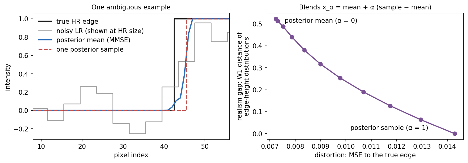
This toy is the thread of the chapter: MSE-trained networks target the posterior mean, while L1-trained networks target coordinate-wise medians. Both choose a central prediction rather than describe all possible answers. Perceptual and adversarial losses favour plausible-looking detail; stochastic diffusion models can generate different candidates. Evaluation must distinguish fidelity, realism and uncertainty.
What the low-resolution image has lost: the frequency view
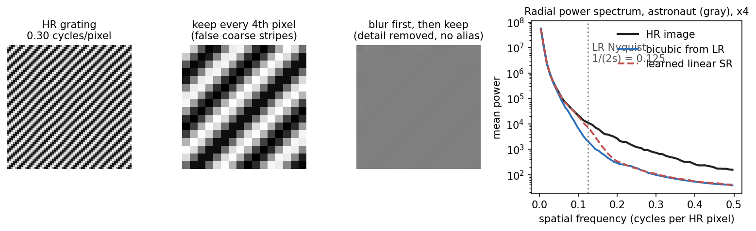
Plain version. Downsampling can alias fine patterns and weaken surviving detail. SR must both restore weakened structure and infer information the input no longer determines.
The LR grid can only represent frequencies up to the LR Nyquist limit, cycles per HR pixel (0.125 at ), where is the scale factor. Higher HR frequencies either fold onto lower ones (aliasing, IP 04) or, if the blur removed them first, vanish. So content above the limit must be unfolded or invented with a prior, and content below it, weakened by the blur, must be restored (Figure 2).
Optional: Aliasing in the LR spectrum (in the Supplementary notes). It writes the folding as a formula and works through the grating of Figure 2.
The benchmark setting: a known degradation
Question. How are training and test pairs made in non-blind SR, and how do we measure the result? Short answer: shrink HR images with one fixed, known operator, and compare the enlarged result with the original by PSNR on the luminance channel.
Most SR benchmarks create LR images with MATLAB’s imresize at its default settings, which use bicubic interpolation and, when shrinking, an anti-aliasing filter that is on by default [3], [4]. There is no added noise, no camera blur and no compression. This “bicubic” setting is clean and reproducible, which made years of results comparable. A model trained on it has learned to invert exactly that one operator.
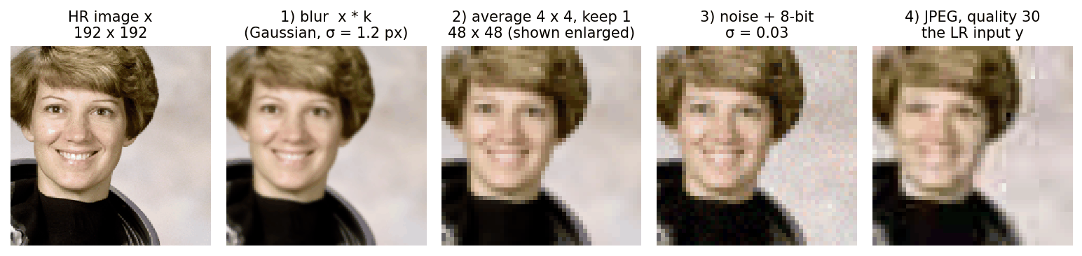
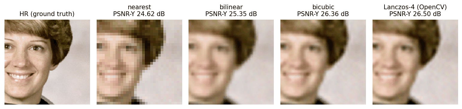
Our running example uses a different but equally known operator, written out step by step: a Gaussian blur with σ = 1.2 HR pixels (the lens), the average of each block (one larger sensor pixel), a little Gaussian noise (σ = 0.01) and rounding to 8 bits. The snippet enlarges the result with four standard interpolators and reports PSNR as SR papers do, on the luminance (Y) channel with a border of pixels removed (see Evaluating SR).
Code · Python · 32 lines
import numpy as np, cv2
from scipy import ndimage as ndi
from skimage import data, img_as_float64

def degrade(hr, s=4, blur=1.2, noise=0.01, rng=None):
    """hr: (H, W, 3) in [0, 1], H and W divisible by s. Returns the LR image y."""
    rng = rng or np.random.default_rng(0)
    x = ndi.gaussian_filter(hr, sigma=(blur, blur, 0))          # 1) lens blur
    H, W, C = x.shape
    x = x.reshape(H // s, s, W // s, s, C).mean(axis=(1, 3))      # 2) s x s pixel integration + decimation
    x = x + noise * rng.standard_normal(x.shape)                  # 3) sensor noise
    return np.round(np.clip(x, 0, 1) * 255) / 255                 # 4) 8-bit quantization

def y_channel(rgb):
    """BT.601 luma on the [16, 235] scale (the MATLAB rgb2ycbcr convention)."""
    return 16 + rgb @ np.array([65.481, 128.553, 24.966])

def psnr(a, b, shave, peak):
    if shave:
        a, b = a[shave:-shave, shave:-shave], b[shave:-shave, shave:-shave]
    return 10 * np.log10(peak**2 / np.mean((a - b) ** 2))

hr = img_as_float64(data.astronaut())                             # (512, 512, 3)
lr = degrade(hr)                                                  # (128, 128, 3)
print("LR shape:", lr.shape)
for name, flag in [("nearest", cv2.INTER_NEAREST), ("bilinear", cv2.INTER_LINEAR),
                   ("bicubic", cv2.INTER_CUBIC), ("lanczos", cv2.INTER_LANCZOS4)]:
    sr = cv2.resize(lr, (512, 512), interpolation=flag)
    sr = np.clip(sr, 0, 1)
    y_hr, y_sr = y_channel(hr), y_channel(sr)
    print(f"{name:8s}  Y, shave 4: {psnr(y_hr, y_sr, 4, 255):.2f} dB | "
          f"Y, no shave: {psnr(y_hr, y_sr, 0, 255):.2f} dB | RGB, shave 4: {psnr(hr, sr, 4, 1):.2f} dB")
Output
LR shape: (128, 128, 3)
nearest   Y, shave 4: 24.62 dB | Y, no shave: 24.66 dB | RGB, shave 4: 23.06 dB
bilinear  Y, shave 4: 25.35 dB | Y, no shave: 25.40 dB | RGB, shave 4: 23.83 dB
bicubic   Y, shave 4: 26.36 dB | Y, no shave: 26.40 dB | RGB, shave 4: 24.81 dB
lanczos   Y, shave 4: 26.50 dB | Y, no shave: 26.54 dB | RGB, shave 4: 24.94 dB
The ranking is the same under every protocol, but Y and RGB differ by about 1.5 dB, so only compare numbers measured the same way.
Real photos go through more than this; Figure 3 adds JPEG compression to the chain. Non-blind SR fixes the whole chain in advance. When it is unknown or varies from photo to photo, the problem becomes blind or real-world SR (DLCV 09A.1).
Classical baselines
Question. What can be done without a deep network, and why is it not enough? Short answer: interpolation spreads the existing samples with a fixed filter; learned linear filters add some lost detail back; neither can model the variety of natural images.
Interpolation: a fixed linear filter
Interpolation places the LR samples on the HR grid and fills the gaps with a weighted sum of nearby samples. In one dimension,
where is an HR pixel index, an LR pixel index, the interpolation kernel and the half-pixel terms align the centers of LR and HR pixels (the convention OpenCV uses). In 2-D the kernel is applied along rows and then columns. IP 02 derives the common kernels:
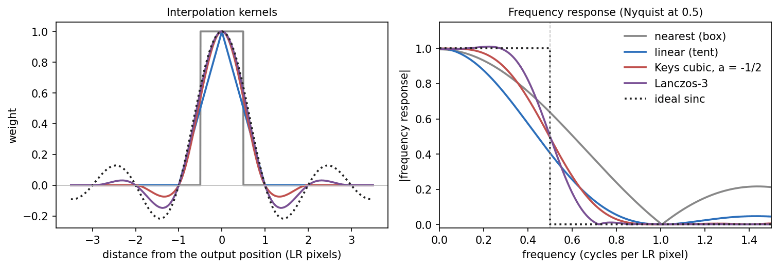
- Nearest neighbor and linear: a box of width 1 (blocky) and a triangle of width 2 (soft).
- Cubic convolution (Keys) [5]: a piecewise cubic of width 4 with a free parameter ; Keys showed that gives the best approximation order in that family. Its small negative lobes sharpen edges slightly. OpenCV’s
INTER_CUBICuses instead (Exercise 1). - Lanczos: for and 0 otherwise, with and the number of lobes kept on each side [6]; OpenCV’s
INTER_LANCZOS4uses .
Wider kernels approximate the ideal sinc better (Figure 4), which is why Lanczos scored highest above (26.50 dB versus 26.36 dB for bicubic). These fixed-kernel interpolators apply the same linear reconstruction rule to an edge and a flat region (away from boundary effects). They cannot identify the missing true HR frequencies from the LR samples alone. Finite kernels can nevertheless introduce spectral replicas and ringing; an output containing high frequencies is not proof that the original detail was recovered (Figure 5).
Learning from examples: from patch pairs to linear filters
Plain version. Learn patch mappings from paired examples, then use precomputed linear corrections to restore similar patches efficiently.
Example-based methods took (LR patch, HR patch) pairs from training images [7] or from the input itself, because small patches recur across scales of one image [8]; sparse coding compressed the pairs into two matched dictionaries [9]. Anchored neighborhood regression (ANR) and A+ replaced the search by precomputed ridge regressors [10], [11], and RAISR learned one filter per bucket of gradient angle, strength and coherence [12]. The common structure is
where is an LR patch, its feature vector, the class (atom or hash bucket) it belongs to, the HR detail to predict, the training pairs of class stacked as the rows of and , the ridge weight and the Frobenius norm.
Optional: Example-based SR and sparse coding in detail (in the Supplementary notes). It gives the sparse-coding objective and the internal-learning idea behind ZSSR.
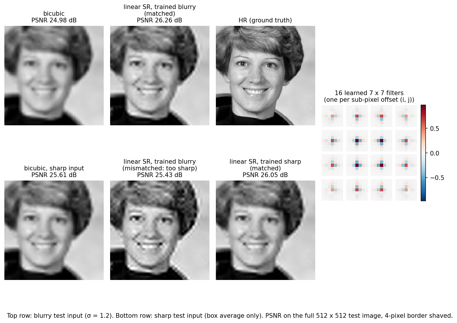
The snippet implements the simplest version, one class, on the running example in grayscale. For every LR pixel it takes the LR patch around it (mean removed, plus a bias) and predicts the block of HR residual (HR image minus its bicubic upsampling). Predicting values per LR pixel and arranging them into an block is what a sub-pixel convolution does (Decision 2), so this is a one-layer, linear version of the networks that follow. We train it on eleven other skimage images, once for “sharp” LR inputs (block averaging only) and once for “blurry” ones (blur σ = 1.2, then averaging), and test both on the astronaut.
Code · Python · 53 lines
import numpy as np, cv2
from numpy.lib.stride_tricks import sliding_window_view
from scipy import ndimage as ndi
from skimage import data, img_as_float64
from skimage.color import rgb2gray

s, p = 4, 7                                     # scale factor, LR patch size

def degrade(x, blur):                           # blur (optional) -> s x s average
    x = ndi.gaussian_filter(x, blur) if blur else x
    H, W = x.shape[0] // s * s, x.shape[1] // s * s
    return x[:H, :W].reshape(H // s, s, W // s, s).mean(axis=(1, 3))

def bicubic(lr):
    return cv2.resize(lr, None, fx=s, fy=s, interpolation=cv2.INTER_CUBIC)

def features(lr):                               # one p x p patch per LR pixel, mean removed, plus a bias
    f = sliding_window_view(np.pad(lr, p // 2, mode="reflect"), (p, p)).reshape(lr.size, p * p)
    return np.c_[f - f.mean(axis=1, keepdims=True), np.ones(lr.size)]

def to_blocks(r):                               # HR residual -> one s*s vector per LR pixel (space-to-depth)
    h, w = r.shape[0] // s, r.shape[1] // s
    return r.reshape(h, s, w, s).transpose(0, 2, 1, 3).reshape(h * w, s * s)

def from_blocks(b, h, w):                       # inverse: depth-to-space (pixel shuffle)
    return b.reshape(h, w, s, s).transpose(0, 2, 1, 3).reshape(h * s, w * s)

def train(images, blur, lam=1e-3):
    A, B = [], []
    for im in images:
        im = im[: im.shape[0] // s * s, : im.shape[1] // s * s]
        lr = degrade(im, blur)
        A.append(features(lr)); B.append(to_blocks(im - bicubic(lr)))
    A, B = np.concatenate(A), np.concatenate(B)
    return np.linalg.solve(A.T @ A + lam * np.eye(A.shape[1]), A.T @ B)   # ridge: (p*p+1, s*s)

def super_resolve(lr, Wt):
    return bicubic(lr) + from_blocks(features(lr) @ Wt, *lr.shape)

def psnr(a, b):
    a, b = a[s:-s, s:-s], b[s:-s, s:-s]          # shave s border pixels
    return 10 * np.log10(1.0 / np.mean((a - np.clip(b, 0, 1)) ** 2))

train_imgs = [img_as_float64(im) for im in (data.camera(), data.moon(), data.coins(), data.page(),
              data.text(), data.brick(), data.grass(), data.gravel(),
              rgb2gray(data.coffee()), rgb2gray(data.chelsea()), rgb2gray(data.rocket()))]
models = {"trained sharp": train(train_imgs, 0.0), "trained blurry": train(train_imgs, 1.2)}
test = img_as_float64(rgb2gray(data.astronaut()))           # never seen in training
print("weights per model:", models["trained sharp"].shape)
for name, blur in [("sharp", 0.0), ("blurry", 1.2)]:
    lr = degrade(test, blur)
    row = "  ".join(f"{m} {psnr(test, super_resolve(lr, W)):.2f}" for m, W in models.items())
    print(f"test {name:6s} | bicubic {psnr(test, bicubic(lr)):.2f} | {row}  (dB)")
Output
weights per model: (50, 16)
test sharp  | bicubic 25.61 | trained sharp 26.05  trained blurry 25.43  (dB)
test blurry | bicubic 24.98 | trained sharp 25.66  trained blurry 26.26  (dB)
Each model has only weights, fitted in closed form in about a second. With the matching degradation it gains 0.44 dB (sharp inputs) and 1.28 dB (blurry inputs) over bicubic on an unseen image. The off-diagonal entries show the price of a wrong assumption: the blurry-trained model over-sharpens sharp inputs and falls below bicubic (25.43 dB versus 25.61 dB), and the sharp-trained model under-corrects blurry ones (25.66 dB versus 26.26 dB). This is the core limitation of non-blind SR: a model is only as good as its degradation assumption. Efrat et al. found the same for classical methods: an accurate blur model matters more than a sophisticated image prior [13]. Figure 6 shows the crops and the 16 learned filters, one per sub-pixel offset.

 BicubicLinear SR (matched)
Deep SR networks: a story of design decisions
Question. A deep SR network is a much richer, non-linear version of the regressor above. How did the field get from a three-layer CNN to today’s transformers, and why does each piece exist? Short answer: through six decisions, each made to fix a specific problem of the previous design, and each with a cost.
Table 1 is the map of this section; each row is explained below in the same order.
| Decision | Landmark model | Problem it solved | What it cost |
|---|---|---|---|
| 1. Learn the mapping end to end, after bicubic upsampling | SRCNN [14] | hand-designed patch pipelines | every layer runs at HR size |
| 1. Upsample at the end instead | FSRCNN [15], ESPCN [16] | the cost of working at HR size | one upsampling tail per scale |
| 2. Upsample with sub-pixel convolution (pixel shuffle) | ESPCN [16] | the cost of a learned upsampler | checkerboard risk at initialization |
| 3. Go deep and predict only the residual | VDSR [17] | slow, unstable training of deep networks | deeper bodies still cost computation and activation memory |
| 4. Remove batch normalization, scale residuals | EDSR [18] | BN’s memory and its normalized feature range | needs residual scaling to train wide models |
| 5. Reweight channels (channel attention), residual in residual | RCAN [19] | all channels treated equally; training 400+ layers | depth makes inference slow |
| 6. Let pixels attend to content far away | SwinIR [20], HAT [21] | fixed, local convolution weights | memory and runtime of attention |
These networks use pixel losses: squared error targets a conditional mean, while L1 targets a coordinate-wise conditional median. Their deterministic outputs do not represent the entire conditional distribution. Architectural improvements can improve a predictor without changing this statistical objective; the next section changes the loss instead.
Decision 1: where to upsample
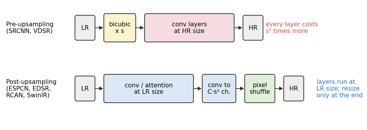
Plain version. The output is times larger than the input in each direction, so somewhere the network must grow the image. If it grows first, every later layer works on times more pixels. If it grows last, every layer works on the small image.
SRCNN, the first end-to-end CNN for SR, enlarges the input with bicubic interpolation and then applies three convolution layers that its authors read as patch extraction, non-linear mapping and reconstruction, the same three steps as sparse-coding SR [14]. This pre-upsampling design is simple, and one network can serve several scales because the interpolation already did the resizing (VDSR trained one network for ×2, ×3 and ×4 this way [17]). Its cost follows from a count. A convolution with input and output channels on an map needs
multiply-accumulates, where is the spatial size of the feature map. The count is proportional to , so running the same layer at HR size costs exactly times more.
Code · Python · 11 lines
def conv_macs(h, w, c_in, c_out, k=3):
    """Multiply-accumulates of one k x k convolution on an h x w feature map."""
    return h * w * c_in * c_out * k * k

s, H, W, C = 4, 128, 128, 64                    # x4 SR of a 128 x 128 input, 64 feature channels
body_pre = conv_macs(s * H, s * W, C, C)        # one body layer at HR size (pre-upsampling)
body_post = conv_macs(H, W, C, C)               # the same layer at LR size (post-upsampling)
tail = conv_macs(H, W, C, 3 * s * s)            # sub-pixel tail: 64 -> 3*s*s channels, then pixel shuffle
print(f"one body layer, pre-upsampling : {body_pre / 1e9:.2f} GMAC")
print(f"one body layer, post-upsampling: {body_post / 1e9:.2f} GMAC (ratio {body_pre / body_post:.0f})")
print(f"sub-pixel tail, 64 -> 48 channels at LR size: {tail / 1e9:.2f} GMAC")
Output
one body layer, pre-upsampling : 9.66 GMAC
one body layer, post-upsampling: 0.60 GMAC (ratio 16)
sub-pixel tail, 64 -> 48 channels at LR size: 0.45 GMAC
For our 128 × 128 example at ×4, one 64-channel layer costs 9.66 GMAC at HR size and 0.60 GMAC at LR size, and networks have tens of such layers. Post-upsampling therefore keeps the body at LR size and enlarges only at the end. FSRCNN did this with a learned transposed convolution (and a thinner mapping stage) and reported a speed-up of more than 40 times over the larger SRCNN-Ex in its C++ Intel i7 CPU comparison [15]. The price is that the tail is tied to one scale factor, so multi-scale models keep one tail per scale; EDSR’s multi-scale variant MDSR shares one body across ×2, ×3 and ×4 [18]. Almost every later network uses post-upsampling (Figure 7).
Decision 2: how to upsample: transposed or sub-pixel convolution
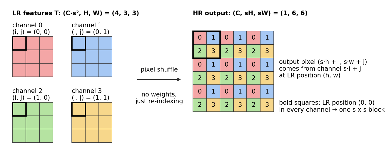
Plain version. A learned upsampler must produce output pixels for every input pixel. A transposed convolution spreads each input pixel over the output with a learned stamp. A sub-pixel convolution computes the values as separate channels at low resolution and then simply rearranges them into an block.
A transposed convolution with stride inserts zeros between neighbouring LR samples and then convolves; equivalently, every LR pixel adds a scaled copy of the kernel to the output, with copies pixels apart. ESPCN observed that each output pixel then uses only some of the kernel’s taps, and the pattern of used taps depends only on the sub-pixel offset (the output position modulo ). There are exactly patterns, so the operation equals ordinary convolutions at LR size, one per offset, with interleaved outputs [16]. ESPCN implements this directly: the last convolution produces channels at LR resolution, and a fixed rearrangement, pixel shuffle (or depth-to-space), turns them into channels at times the resolution. The rearrangement has no parameters, and EDSR, RCAN, SwinIR and HAT all use it [18], [19], [20], [21].
The precise version is an index rule. Let be the LR feature tensor of shape and the output of shape . Then
where is the output channel, an LR position and the sub-pixel offset inside the output block that belongs to that LR position. In words: the channels that belong to output channel are read in row-major order of and spread over one block. This is the ordering of PyTorch’s PixelShuffle, whose implementation reshapes the channel axis into and permutes it next to the height and width axes [22]. The inverse, space-to-depth (pixel unshuffle), reads each block back into channels; efficient networks use it at the input to work at a lower resolution. Figure 8 draws the rule for .
The NumPy version writes pixel shuffle and its inverse as one reshape, one transpose and one reshape each, checks the index rule element by element, and checks that the two operations are exact inverses.
Code · Python · 27 lines
import numpy as np

def pixel_shuffle(t, s):
    """Depth-to-space: (C*s*s, H, W) -> (C, H*s, W*s)."""
    Cs2, H, W = t.shape
    C = Cs2 // (s * s)
    return t.reshape(C, s, s, H, W).transpose(0, 3, 1, 4, 2).reshape(C, H * s, W * s)

def pixel_unshuffle(x, s):
    """Space-to-depth: (C, H*s, W*s) -> (C*s*s, H, W)."""
    C, Hs, Ws = x.shape
    H, W = Hs // s, Ws // s
    return x.reshape(C, H, s, W, s).transpose(0, 2, 4, 1, 3).reshape(C * s * s, H, W)

rng = np.random.default_rng(0)
s, C, H, W = 3, 2, 4, 5
t = rng.standard_normal((C * s * s, H, W))
x = pixel_shuffle(t, s)
print(x.shape)                                                   # (2, 12, 15)

# The index rule: output (c, s*h + i, s*w + j) comes from channel c*s*s + s*i + j at (h, w).
ok = all(x[c, s*h + i, s*w + j] == t[c*s*s + s*i + j, h, w]
         for c in range(C) for h in range(H) for w in range(W)
         for i in range(s) for j in range(s))
print("index rule holds:", ok)
print("unshuffle(shuffle(t)) == t:", np.array_equal(pixel_unshuffle(x, s), t))
print("shuffle(unshuffle(x)) == x:", np.array_equal(pixel_shuffle(pixel_unshuffle(x, s), s), x))
Output
(2, 12, 15)
index rule holds: True
unshuffle(shuffle(t)) == t: True
shuffle(unshuffle(x)) == x: True
So, when the kernel size is a multiple of , the two upsamplers represent the same operations; they differ in cost and behaviour. Pixel shuffle is a permutation of array entries: exactly invertible, with the inverse permutation as its gradient, and nothing is computed at HR size. Its one weakness is shared with the transposed convolution: each sub-pixel offset has its own filter, so a freshly initialized layer responds unequally at the offsets and a flat input comes out as a checkerboard. Aitken et al. initialize the filters as copies of one filter, so the layer starts as a convolution followed by nearest-neighbor upsampling, which removes the pattern [23]; DLCV 01B works through the cause with code. Our linear regressor is a one-layer sub-pixel convolution: its 16 filters in Figure 6 are the 16 offsets.
Decision 3: how deep, and why predict a residual
Plain version. Deeper networks capture wider context but are harder to optimize. Residual learning predicts a correction to a simple upsampled input.
VDSR made the network much deeper than SRCNN (20 weight layers of filters) and made that depth trainable with two choices [17]. First, global residual learning: the network predicts only the correction to the interpolated input,
where is bicubic upsampling, takes the upsampled HR-sized image, is the SR output and is the training loss for one pair. Second, a very high learning rate kept stable by adjustable gradient clipping [17].
Optional: Adjustable gradient clipping (in the Supplementary notes). It gives VDSR’s clipping rule and why it scales with the learning rate.
Why does the residual help? The interpolated image already contains the low frequencies, so the target is small and centred at zero. The snippet measures this on the running example.
Code · Python · 12 lines
import numpy as np, cv2
from scipy import ndimage as ndi
from skimage import data, img_as_float64
from skimage.color import rgb2gray

s = 4
hr = img_as_float64(rgb2gray(data.astronaut()))                        # (512, 512), values in [0, 1]
lr = ndi.gaussian_filter(hr, 1.2).reshape(128, s, 128, s).mean(axis=(1, 3))   # the running example
up = cv2.resize(lr, None, fx=s, fy=s, interpolation=cv2.INTER_CUBIC)   # bicubic upsampling
r = hr - up                                                            # what a residual network predicts
print(f"HR image: mean {hr.mean():.3f}  std {hr.std():.3f}")
print(f"residual: mean {r.mean():+.3f}  std {r.std():.3f}  |r| < 0.05 at {np.mean(np.abs(r) < 0.05):.0%} of pixels")
Output
HR image: mean 0.442  std 0.296
residual: mean -0.000  std 0.056  |r| < 0.05 at 82% of pixels
The residual has about one fifth of the image’s standard deviation and is below 0.05 at 82% of the pixels. A network whose output starts near zero is thus already close to a sensible answer (bicubic) and can spend its capacity on edges and textures. Post-upsampling networks keep the idea in two forms: local residual blocks inside the body (DLCV 01B compares them with ResNet’s), and a long skip from the first features to the last. A matching-shape skip addition is cheap relative to the convolutional body, and later networks in Table 1 retain residual paths; increasing the body depth itself is not free.
Decision 4: remove batch normalization
Plain version. Batch normalization (BN) rescales every feature channel to a standard range, which helps classifiers. An SR network must reproduce exact intensities, so this throws away something it needs, and EDSR uses the memory saved by removing BN for a wider network.
A BN layer normalizes each channel with the mean and variance of the current mini-batch during training, then applies a learned scale and shift; at test time it uses running averages. SRResNet, the generator of SRGAN, used residual blocks with BN, as classifiers did [24]. EDSR removed them, for two reasons [18]: BN normalizes the features and so takes away the network’s range flexibility, and BN layers use as much memory as the convolutions before them (without BN, training used about 40% less memory than SRResNet). The savings went into width: 32 residual blocks with 256 channels in the full EDSR model. At that width training became numerically unstable, which EDSR fixed with residual scaling: each residual branch is multiplied by 0.1 before it is added. EDSR also switched to the L1 loss (it converged better), initialized its ×3 and ×4 models from the ×2 model, and won the NTIRE 2017 SR challenge [18], [25]. ESRGAN later added a third reason: when training and test statistics differ, BN tends to introduce artifacts, especially in deep GAN-trained networks [26].
The cost: the network loses BN’s help with optimization and needs residual scaling and careful initialization instead. And at deployment, BN-free networks have activations with a much larger dynamic range, which makes them harder to quantize (DLCV 01C). DLCV 01B discusses when to leave normalization out in general.
Decision 5: reweight channels (RCAN)
Plain version. Some feature channels carry smooth, low-frequency content that the input already shows; others carry the fine detail SR is really about. Channel attention lets the network turn each channel up or down depending on the image, instead of treating all channels the same.
RCAN made two changes [19]. Its channel attention summarizes each channel by its average, passes the summary through a small bottleneck, and uses the result to rescale the channel. For a feature tensor with channels of size ,
where is the value of channel at position , the vector of channel averages, a convolution that reduces channels to , the ReLU, a convolution that expands them back to , the sigmoid, the weight of channel , and the rescaled channel. RCAN uses and reduction ratio , so the bottleneck has 4 channels; the extra parameters are tiny. The same mechanism appears in classification networks as squeeze-and-excitation (DLCV 01B).
Its residual-in-residual structure makes great depth trainable: 10 residual groups of 20 channel-attention blocks, each group with a short skip connection, all inside one long skip connection, for over 400 layers [19]. The authors’ argument is that the abundant low-frequency information of the input can bypass the body through these skips, so the main network can focus on high frequencies. The cost is latency: 400 layers run one after another.
Decision 6: let pixels attend to content far away (SwinIR, HAT)
Plain version. A convolution applies the same weights everywhere; self-attention computes its weights from the content, so a pixel on one window frame can borrow detail from a similar frame elsewhere. Full attention over an image is too expensive, so SR transformers attend within small windows that shift between layers.
Within a window of tokens (here, one token per LR pixel), self-attention computes
where , and are the query, key and value matrices obtained by linear maps of the tokens in the window ( rows each), is the dimension of a query or key, and is a learned bias that depends only on the relative position of two tokens [21]. Each output is a weighted average of the values in the window, weighted by how well its query matches each key (ML 05 explains attention and shifted windows in general). Windows are what make this affordable. For a map of tokens with channels, the Swin Transformer paper counts
where MSA is global multi-head self-attention, W-MSA attention within windows, the first term the linear projections and the second the attention itself [27]. Global attention grows with the square of the number of tokens; windowed attention grows linearly. With SwinIR’s width and window on our 128 × 128 LR map, the formulas give about 98.8 GMAC for global attention and 2.50 GMAC for windows in one layer (our arithmetic; Exercise 6).
SwinIR builds an SR network around this block: a convolution for shallow features, residual Swin Transformer blocks (several Swin layers plus a convolution, wrapped in a residual connection; 6 blocks of 6 layers, windows of 8 and 180 channels in its standard SR setting), and a pixel-shuffle reconstruction, trained with the L1 loss [20]. HAT asked how much of the input SwinIR really uses. With an attribution method for SR (LAM), its authors found that SwinIR uses a limited spatial range, and designed HAT to “activate more pixels” [21]: a channel-attention branch in parallel with window attention, windows of 16, an overlapping cross-attention block whose keys and values come from larger, overlapping windows, and pre-training on ImageNet for the same SR task before fine-tuning on DIV2K and Flickr2K. Later backbones continue the search for cheap long-range context: DAT alternates spatial and channel self-attention [28], and MambaIR replaces attention with state-space scans that reach the whole image at linear cost [29].
The cost is memory and runtime, which grow with the window size; large images are processed in tiles, which can leave seams. And Table 1’s main point still holds: trained with L1, these networks owe their sharper outputs to better use of context, not to sampling.
The common training recipe. These networks are trained on small random crops from DIV2K or DIV2K plus Flickr2K (EDSR used LR patches), with random flips and 90° rotations, the L1 loss and Adam. A ”+” after a name (EDSR+) means geometric self-ensemble: the outputs for the 8 flipped and rotated versions of the input are transformed back and averaged [18]. The general losses are in DLCV 09.
Perceptual and adversarial SR
Question. If a pixel loss favours a central estimate rather than one sharp candidate, can a different loss produce realistic detail? Short answer: yes, by rewarding outputs that look like real photos (perceptual and adversarial losses), at the price of a lower PSNR and occasional invented detail.
Perceptual losses and GANs
Johnson, Alahi and Fei-Fei trained SR networks with a perceptual loss, the distance between features of a pretrained classifier (VGG [30]) for the output and for the target, and obtained sharper edges and textures than with a pixel loss, at a lower PSNR [31]. SRGAN added an adversarial loss: a discriminator learns to tell SR outputs from real HR images, and the SR network (SRResNet, 16 residual blocks) is trained to fool it, which pushes the solution toward the natural image manifold; in a mean-opinion-score test, raters clearly preferred SRGAN’s outputs [24]. ESRGAN improved each part: residual-in-residual dense blocks without BN (Decision 4), a relativistic discriminator that judges whether a real image looks more realistic than a generated one, and a perceptual loss on VGG features taken before the activation; a variant won region 3 (the most perceptual one) of the PIRM 2018 challenge [26], [32]. A typical generator loss is
where is the SR output, the HR target, a fixed layer of a pretrained network, the adversarial term computed with the discriminator, and weights chosen by hand. GANs are explained in ML 07.
ESRGAN also introduced a simple knob, network interpolation: blend the weights of a PSNR-oriented network and its GAN-fine-tuned copy, with , to move between smooth and textured outputs without retraining [26].
Optional: ESRGAN’s changes in detail (in the Supplementary notes). It gives the relativistic discriminator’s losses, the reasons for features before activation, and the block structure.
The perception–distortion trade-off
Blau and Michaeli defined distortion as the expected dissimilarity between and (MSE, for example) and perceptual quality as the distance between the distribution of outputs and the distribution of real images, and formalized the frontier between the two objectives [2]. As the permitted distortion shrinks, the best achievable perceptual quality cannot improve; with an ambiguous posterior, the low-distortion MMSE solution can have an unrealistic output distribution. The conflict is not inevitable in a noiseless, invertible problem where the input identifies the HR image exactly. The formal statement is in DLCV 09. Our toy traces such a curve (Figure 1, right): moving from the posterior mean toward a posterior sample raises MSE from 0.0072 to 0.0143 and closes the realism gap. ESRGAN’s network interpolation is an empirical way to explore operating points. Blending nonlinear network parameters is not the same operation as interpolating the toy’s output images, and is not guaranteed to trace the theoretical optimum. Two practical consequences follow:
- A method should state where on the trade-off it aims. Comparing a GAN to an MSE network by PSNR alone, or by a perceptual metric alone, says nothing about which is better.
- Benchmarks must measure both axes. The PIRM 2018 challenge did this by splitting the perception–distortion plane into three regions by RMSE (at most 11.5, 12.5 and 16) and ranking methods within each region by a perceptual index built from two no-reference metrics, NIQE [33] and the SR-specific metric of Ma et al. [34], [32].
Diffusion SR for a known degradation
Question. Can a model represent several plausible HR answers rather than just a central prediction? Short answer: conditional diffusion learns an approximation to the conditional image distribution and can sample different candidates, at the cost of iterative inference. A trained sampler does not certify exact Bayesian posterior sampling or exact data consistency.
A diffusion model learns to turn noise into realistic images step by step; conditioned on the LR image, it generates an HR image that fits the input, and different random seeds give different plausible answers. SR3 is the representative method for the non-blind setting, with LR images made by bicubic downscaling [35]. Its U-Net [36] receives the noisy HR estimate concatenated, along the channel axis, with the bicubic upsampling of the LR image, and learns to remove noise at many levels. Inference starts from pure Gaussian noise and refines it, in at most 100 steps in the paper’s setting [35].
SR3’s own comparisons show the trade-off of the previous section. On ×8 face SR (16 × 16 to 128 × 128), human raters asked to pick the real photo chose SR3’s output close to 50% of the time, while GAN baselines reached at most 34%. On ×4 ImageNet SR, a regression model with the same architecture scored higher PSNR and SSIM, while SR3 scored better on sample-quality metrics; the authors note that PSNR and SSIM penalize any synthetic detail that is not perfectly aligned [35]. SR3 also checked consistency: its outputs, downsampled again, matched the LR inputs better than the GAN baselines’ outputs did [35]. DLCV 09B explains how such a conditional diffusion restorer is trained and sampled, and ML 08 the diffusion mechanics.
Diffusion can generate plausible detail that does not align with the paired target, lowering PSNR even when viewers prefer it; lower PSNR is not a universal guarantee for every model or setting. Generated details can be wrong (see Failure modes), and iterative sampling costs many network evaluations. Methods built on large pretrained text-to-image models, with sampling cut to a few steps or one, were developed for real-world photos and are covered in DLCV 09A.1.
When the degradation is unknown: blind and real-world SR
Plain version. Everything so far assumed that we know how the small image was made. A real photo comes with its own unknown blur, noise and compression, and a model trained on bicubic pairs misjudges it, as the mismatched linear model above did. Blind and real-world SR either trains on a very wide range of synthetic degradations, estimates the degradation first, or learns from real captured pairs, and it evaluates results without ground truth. These methods, their datasets, and the diffusion-prior restorers used for real photos have their own chapter, DLCV 09A.1 · Blind and Real-World Image Super-Resolution.
Arbitrary-scale SR
Plain version. The networks above are trained for one fixed factor such as ×4. Arbitrary-scale networks treat the image as a continuous function, so you can ask for any output size, including non-integer factors like ×2.7.
Meta-SR replaced the fixed upsampling tail with a meta-upscale module that predicts the weights of the upscaling filters from the scale factor and the relative position of each output pixel [37]. LIIF went further and learned a local implicit image function [38]:
where is a continuous query coordinate in the image plane, the latent feature vector (from a CNN encoder applied to the LR image) whose grid position is nearest to , and a small MLP that outputs the RGB value at . Because is continuous, the same network renders any output size. Trained on scales between ×1 and ×4, it was shown producing outputs up to ×30 [38]. The price is one MLP evaluation per output pixel, and queries far outside the training scales rely on learned assumptions rather than additional measured detail.
Optional: LIIF’s three refinements (in the Supplementary notes). It explains feature unfolding, local ensemble and cell decoding.
Efficiency
Plain version. Many SR uses (phones, video calls, game rendering) need results in milliseconds on small chips. Efficient SR asks how small and fast a network can be while staying above a quality threshold.
Post-upsampling with pixel shuffle (Decisions 1 and 2) is the first rule: almost all computation happens at LR size. Beyond that, efficient networks reuse features cheaply; IMDN, for example, splits features step by step into a “distilled” part that is kept and a part that is processed further, then fuses them with a contrast-aware channel attention [39]. Parameters, FLOPs and runtime measure different costs, so the NTIRE efficient SR challenges score all three. In 2024 and 2025 the task was ×4 SR, and entries had to reach a PSNR of at least 26.90 dB on the validation set and 26.99 dB on the test set while minimizing runtime, parameters and FLOPs [40], [41]. Compressing an existing network (pruning, quantization, distillation) is the subject of DLCV 01C.
Evaluating SR
Question. How do you tell whether one SR result is better than another? Short answer: for fidelity, follow the community’s fixed PSNR/SSIM recipe exactly, because small details change the numbers; for realism, add perceptual metrics and human judgments, and never compare the two kinds by one number. The generic metrics are explained in DLCV 09; this section covers what is specific to SR.
Y-channel PSNR and SSIM with border shaving
The classical protocol, inherited from the MATLAB code of early papers, is:
- Convert both the HR image and the SR output to YCbCr and keep the luma channel
where are the (gamma-encoded) color values and lies in . These are the BT.601 coefficients as implemented by MATLAB’s rgb2ycbcr (and by skimage.color.rgb2ycbcr) [42], [43].
2. Remove a border of pixels from both images before comparing (“shaving”), so that the effects of padding at the image border do not dominate.
3. Compute PSNR with peak value 255 and SSIM [44] on what remains. Definitions are in DLCV 09.
The details vary even within one paper. EDSR reports its benchmark results on Y with a border equal to the scale factor, but its ablation study on DIV2K uses all RGB channels and ignores border pixels [18]; the NTIRE 2024 and 2025 ×4 challenges compute on Y with a 4-pixel border [45], [46]. Wang et al. note that the color space and channel alone can change results by up to 4 dB in one reported case [4]. Part of that is arithmetic: the coefficients above sum to 219, so with , and PSNR with peak 255 on adds dB to PSNR on with peak 1 (Exercise 2). Rounding, clipping and the resizer also shift results slightly, so fair comparisons run every method through one evaluation script.
The standard test sets
SR papers report results on a small set of public test sets, each with a different character [4]:
| Test set | Images | Content | Source |
|---|---|---|---|
| Set5 | 5 | baby, bird, butterfly, head, woman | [47] |
| Set14 | 14 | people, animals, flowers, comic, slides | [48] |
| BSD100 (B100) | 100 | natural scenes, the test images of the Berkeley segmentation dataset | [49] |
| Urban100 | 100 | buildings and city scenes with regular structures | [50] |
| Manga109 | 109 | Japanese comic volumes (line art and screen tones) | [51], [52] |
| DIV2K validation | 100 | diverse 2K-resolution photos | [53] |
Set5 and Set14 are tiny, so a few hundredths of a dB on them mean little. The sets reward different abilities: Urban100 is full of repeated structures, and HAT’s larger attention window helped most there [21].
Why PSNR and perceptual rankings disagree
Three reasons, all seen in this chapter. First, PSNR is maximized by the blurry average of all plausible answers, so a method that commits to one sharp answer loses PSNR even when it looks better (Figure 1; SR3 versus its regression baseline). Second, a texture with the right statistics but shifted by half a period has a large pixel error. Third, learned perceptual metrics such as LPIPS [54] and no-reference metrics such as NIQE [33] reward natural-looking texture and can be fooled by over-sharpening, while PSNR rewards smoothness. The NTIRE 2025 ×4 challenge ran a restoration track ranked by PSNR and a perceptual track ranked by one combined score of six full-reference and no-reference quality metrics, including LPIPS and NIQE [46]. The advice from DLCV 09 applies: report a fidelity metric, a perceptual metric and, for generative SR, a user study.
Datasets and benchmarks
Plain version. A few datasets and a yearly competition define most of what “state of the art” means in non-blind SR.
- DIV2K [53] contains 1,000 diverse 2K-resolution images, split 800/100/100 for training, validation and testing [46]. It was introduced for the NTIRE 2017 challenge and is the standard training set. It is often combined with Flickr2K, which the NTIRE 2025 report describes as 2,650 2K images [46]; the combination is called DF2K, and HAT, for example, fine-tunes on it after pre-training on ImageNet [21].
- NTIRE 2017 [25], the first SR challenge of the series, had a bicubic track and a track with unknown downscaling operators (learnable from the provided training pairs), each at ×2, ×3 and ×4.
- NTIRE 2024 and 2025 ×4 SR [45], [46] use bicubic ×4 on DIV2K; the 2025 edition added the perceptual track described above.
- NTIRE efficient SR [40], [41] ranks ×4 models by runtime, parameters and FLOPs above a fixed PSNR.
The real-world datasets and challenges, which have no clean bicubic pairs, are described in DLCV 09A.1.
Failure modes
Plain version. An SR model can fail by being too cautious (blurry) or too bold (invented detail). The bold failures are more dangerous, because the result looks convincing.
- Over-smoothing. A central prediction can suppress ambiguous detail, giving waxy skin, flat grass or soft hair. MSE targets a mean; L1 targets a median. Neither statistical objective guarantees blur on every input, but neither asks the network to represent all plausible sharp alternatives (Figure 1).
- Hallucinated text and faces. At large scales a generative model can turn illegible text into legible but wrong characters, or a few pixels of a face into a sharp face that is not the person photographed; for forensic, medical or scientific images this is unacceptable. Ren et al. argue that fidelity and no-reference metrics both capture such hallucinations poorly, and propose scoring them with a multimodal large language model [55].
- Texture artifacts. GAN-based models can add repetitive, noise-like textures; ESRGAN was designed partly to reduce such artifacts of SRGAN [26]. Our mismatched linear model shows halos and exaggerated edges in miniature (Figure 6).
- Color shifts. Diffusion-based SR can shift global colors away from the input; Moser et al. list it among the open problems of diffusion SR [56].
- Degradation mismatch. A non-blind model applied to images made differently under- or over-corrects (Figure 6). Testing on more than one degradation exposes this; DLCV 09A.1 covers the remedies.
- Tiling seams. Large images are often processed in patches; non-overlapping patches can leave visible borders, as the SwinIR authors note for patch-based processing [20].
A useful sanity check for any SR output is consistency with the input: degrade the output with the assumed model and compare it with . A large difference means the model changed content that the LR image did measure.
Modern view
Survey papers
Two surveys cover this chapter’s material. Wang, Chen and Hoi split deep SR into supervised, unsupervised and domain-specific SR, and describe supervised models along independent axes: where to upsample (pre-, post-, progressive, iterative up-and-down), with which operator, which network design (residual, recursive, dense, attention and others), which losses and which training strategies [4]. Their takeaway matches Table 1: most models are combinations of choices along these axes, so read a new model as “which choices did it change?”. The survey also tabulates the test sets; it predates transformers and diffusion models. Moser et al. cover diffusion models for SR: the theory first, then methods organized by input domain (pixel, latent, wavelet), conditioning, guidance, corruption spaces and zero-shot use of pretrained models [56]. Their open issues (high compute, poor comparability across papers, limited explainability, color shifts) are a good checklist for reading any diffusion SR paper. The blind and real-world surveys are discussed in DLCV 09A.1.
State of the art, 2023–2026
- Fidelity-oriented SR uses attention and state-space backbones (HAT, DAT, MambaIR [21], [28], [29]), large-scale pre-training, and is benchmarked each year by the NTIRE ×4 restoration track [45], [46].
- Evaluation is catching up with generation: perceptual SR has its own challenge track with a combined perceptual score, so realism-oriented methods are no longer ranked by PSNR [46], and newer work explicitly evaluates hallucination [55].
- Efficiency has its own benchmark with fixed quality thresholds [40], [41].
Open problems
- Faithful generative SR. How to get diffusion-level realism without inventing content, and how to show a user which details are measured and which are guessed.
- Evaluation. PSNR rewards blur, perceptual metrics can be gamed, and hallucination metrics are new.
- Benchmark saturation. Gains of a few hundredths of a dB on small bicubic test sets say little about real use; the bicubic setting itself is far from real cameras (DLCV 09A.1).
- Cost. Attention and diffusion models are far heavier than the networks of the efficient SR challenges.
- Arbitrary and extreme scales. Behaviour far outside the training scales, and at factors where almost everything is generated, is poorly understood.
Key takeaways
- Known downsampling still loses information; a prior determines unresolved detail.
- MSE favors a conditional mean and L1 a coordinate-wise median; either can smooth uncertain structures.
- Non-blind results depend on the assumed degradation matching the input.
- Late upsampling, residual paths and feature mixing change cost and detail recovery; compare them under the same recipe.
- The perception–distortion frontier does not forbid improving both metrics from a weak baseline; learned generators have no exact-sampling guarantee.
- State color channels and border shaving, check low-resolution consistency, and inspect text, faces, textures and seams.
Exercises
- Which cubic does OpenCV use? Make a 1-D signal of 16 zeros with a single 1 in the middle, upsample it by 4 with
cv2.resize(..., interpolation=cv2.INTER_CUBIC), and compare the result with the Keys kernel evaluated at the half-pixel-aligned positions for and . Then plot both kernels’ frequency responses and compare their values at the LR Nyquist frequency.
Hint
The output of a resize of a unit impulse is the kernel itself, sampled at the output positions. In our run the maximum absolute difference was 0.0 for and about 0.037 for . A more negative gives deeper negative lobes, a response that stays near 1 a little longer and then overshoots slightly: a sharper but more ringing interpolator. Repeat with INTER_LANCZOS4 and the Lanczos kernel with ; the match is close but not exact (we measured a maximum difference of about 0.0016), because the library normalizes the weights.
- Protocol arithmetic. (a) Show that -PSNR with peak 255 equals the PSNR of with peak 1 plus . (b) In the benchmark-setting snippet, change the shave from 4 to 0 and to 16 pixels and explain the size of the change. (c) Why is shaving necessary for a network with zero padding but nearly irrelevant for
cv2.resize?
Hint
(a) , so the MSE scales by and PSNR becomes dB. (b) Shaving changes the result by only a few hundredths of a dB here (24.66 versus 24.62 dB for nearest neighbor), because OpenCV extrapolates borders reasonably and the image edges are smooth. (c) Zero padding makes a convolutional network see black outside the image, so the outputs near the border are systematically worse; shaving removes a region whose quality depends on the padding choice rather than on the method.
- A channel-ordering bug. Suppose one library orders the channels as (our formula) and another as . You load weights trained with the first ordering into the second. For and , which of the 12 channels end up in the right place? What does the output look like?
Hint
Solve with : , so only and coincide, 2 channels out of 12 (we checked this by enumerating all 12). The other values are moved to the wrong color channel and the wrong sub-pixel offset, so the output shows a fine color mosaic in every 2 × 2 block even though the coarse image is recognizable. For the two orderings agree, which is why such bugs often appear only when moving from grayscale to color models.
- Make the linear model better. Starting from the regressor snippet, (a) change the patch size to 3, 5, 9 and 11; (b) split LR pixels into classes by the angle of the local gradient (as RAISR does) and fit one regressor per class; (c) add noise with σ = 0.01 to the LR training images but not to the test images, and the other way round. Report PSNR for each change and explain.
Hint
(a) On the blurry test input we measured 25.94 dB for , 26.18 dB for and 26.26 dB for : beyond 7 × 7 a linear model gains nothing. (b) Four angle classes (computed from the gradient of the slightly smoothed LR image) gave 26.33 dB and eight gave 26.32 dB, a small gain: classes let the filter follow edge direction, which is what makes RAISR and A+ better than one global filter. (c) Training on noisy inputs teaches the model to smooth, so it under-sharpens clean inputs; training on clean inputs teaches it to amplify fine detail, so it amplifies noise. This is the noise version of the blur mismatch in Figure 6.
- Posterior mean by hand. Two HR pixels are independent and equally likely to be 0 or 1. The LR pixel is with no noise. (a) For each value of , give the posterior mean of and a posterior sample. (b) Compute the expected per-pixel MSE of both estimators. (c) Which estimator produces outputs that look like the HR data?
Hint
(a) and determine exactly. For (probability 1/2) the posterior is or with equal probability, so the mean is and a sample is one of the two. (b) Only contributes. The mean has squared error per pixel there, so its MSE is . A sample is right half the time and wrong by 1 on both pixels otherwise, so its MSE is : exactly twice as large. (c) Only the sample: real pixels are 0 or 1, and the value 0.5 never occurs in the HR data.
- The price of global attention. Using the two formulas of Decision 6, compute and for , and LR maps of and tokens. How does the ratio between them change when the image side doubles, and why? What window size would make windowed attention as expensive as global attention?
Hint
We obtained 6.6 versus 0.63 GMAC (ratio 10.5) at and 98.8 versus 2.50 GMAC (ratio 39.5) at . Doubling the side multiplies by 4: the projection term and the windowed attention term grow by 4, but the global attention term grows by 16. The two attention terms are equal when , that is when one window covers the whole image.
References
- S. C. Park, M. K. Park and M. G. Kang, “Super-Resolution Image Reconstruction: A Technical Overview,” IEEE Signal Processing Magazine, vol. 20, no. 3, pp. 21–36, 2003. doi
- Y. Blau and T. Michaeli, “The Perception-Distortion Tradeoff,” in Proc. IEEE/CVF CVPR, 2018, pp. 6228–6237. doi · arXiv
- MathWorks, “imresize: Resize image,” MATLAB documentation (default method bicubic; antialiasing on when shrinking). link
- Z. Wang, J. Chen and S. C. H. Hoi, “Deep Learning for Image Super-Resolution: A Survey,” IEEE TPAMI, vol. 43, no. 10, pp. 3365–3387, 2021. doi · arXiv
- R. Keys, “Cubic Convolution Interpolation for Digital Image Processing,” IEEE Transactions on Acoustics, Speech, and Signal Processing, vol. 29, no. 6, pp. 1153–1160, 1981. doi
- C. E. Duchon, “Lanczos Filtering in One and Two Dimensions,” Journal of Applied Meteorology, vol. 18, no. 8, pp. 1016–1022, 1979. doi
- W. T. Freeman, T. R. Jones and E. C. Pasztor, “Example-Based Super-Resolution,” IEEE Computer Graphics and Applications, vol. 22, no. 2, pp. 56–65, 2002. doi
- D. Glasner, S. Bagon and M. Irani, “Super-Resolution from a Single Image,” in Proc. IEEE ICCV, 2009, pp. 349–356. doi
- J. Yang, J. Wright, T. S. Huang and Y. Ma, “Image Super-Resolution via Sparse Representation,” IEEE Transactions on Image Processing, vol. 19, no. 11, pp. 2861–2873, 2010. doi
- R. Timofte, V. De Smet and L. Van Gool, “Anchored Neighborhood Regression for Fast Example-Based Super-Resolution,” in Proc. IEEE ICCV, 2013, pp. 1920–1927. doi · CVF
- R. Timofte, V. De Smet and L. Van Gool, “A+: Adjusted Anchored Neighborhood Regression for Fast Super-Resolution,” in Computer Vision – ACCV 2014, Lecture Notes in Computer Science, Springer, 2015, pp. 111–126. doi
- Y. Romano, J. Isidoro and P. Milanfar, “RAISR: Rapid and Accurate Image Super Resolution,” IEEE Transactions on Computational Imaging, vol. 3, no. 1, pp. 110–125, 2017. doi · arXiv
- N. Efrat, D. Glasner, A. Apartsin, B. Nadler and A. Levin, “Accurate Blur Models vs. Image Priors in Single Image Super-Resolution,” in Proc. IEEE ICCV, 2013, pp. 2832–2839. doi · CVF
- C. Dong, C. C. Loy, K. He and X. Tang, “Image Super-Resolution Using Deep Convolutional Networks,” IEEE TPAMI, vol. 38, no. 2, pp. 295–307, 2016. doi · arXiv
- C. Dong, C. C. Loy and X. Tang, “Accelerating the Super-Resolution Convolutional Neural Network,” in Proc. ECCV, 2016, pp. 391–407. doi · arXiv
- W. Shi, J. Caballero, F. Huszár, J. Totz, A. P. Aitken, R. Bishop, D. Rueckert and Z. Wang, “Real-Time Single Image and Video Super-Resolution Using an Efficient Sub-Pixel Convolutional Neural Network,” in Proc. IEEE CVPR, 2016, pp. 1874–1883. doi · arXiv
- J. Kim, J. K. Lee and K. M. Lee, “Accurate Image Super-Resolution Using Very Deep Convolutional Networks,” in Proc. IEEE CVPR, 2016, pp. 1646–1654. doi · arXiv
- B. Lim, S. Son, H. Kim, S. Nah and K. M. Lee, “Enhanced Deep Residual Networks for Single Image Super-Resolution,” in Proc. IEEE CVPR Workshops, 2017, pp. 1132–1140. doi · arXiv
- Y. Zhang, K. Li, K. Li, L. Wang, B. Zhong and Y. Fu, “Image Super-Resolution Using Very Deep Residual Channel Attention Networks,” in Proc. ECCV, 2018, pp. 294–310. doi · arXiv
- J. Liang, J. Cao, G. Sun, K. Zhang, L. Van Gool and R. Timofte, “SwinIR: Image Restoration Using Swin Transformer,” in Proc. IEEE/CVF ICCV Workshops, 2021, pp. 1833–1844. doi · arXiv
- X. Chen, X. Wang, J. Zhou, Y. Qiao and C. Dong, “Activating More Pixels in Image Super-Resolution Transformer,” in Proc. IEEE/CVF CVPR, 2023, pp. 22367–22377. doi · arXiv
- PyTorch contributors, “PixelShuffle.cpp” (implementation of
torch.nn.PixelShuffleandtorch.nn.PixelUnshuffle), PyTorch source code. GitHub - A. Aitken, C. Ledig, L. Theis, J. Caballero, Z. Wang and W. Shi, “Checkerboard Artifact Free Sub-Pixel Convolution: A Note on Sub-Pixel Convolution, Resize Convolution and Convolution Resize,” arXiv:1707.02937, 2017. arXiv
- C. Ledig, L. Theis, F. Huszár, J. Caballero, A. Cunningham, A. Acosta, A. Aitken, A. Tejani, J. Totz, Z. Wang and W. Shi, “Photo-Realistic Single Image Super-Resolution Using a Generative Adversarial Network,” in Proc. IEEE CVPR, 2017, pp. 105–114. doi · arXiv
- R. Timofte, E. Agustsson, L. Van Gool, M.-H. Yang, L. Zhang et al., “NTIRE 2017 Challenge on Single Image Super-Resolution: Methods and Results,” in Proc. IEEE CVPR Workshops, 2017, pp. 1110–1121. doi · CVF
- X. Wang, K. Yu, S. Wu, J. Gu, Y. Liu, C. Dong, Y. Qiao and C. C. Loy, “ESRGAN: Enhanced Super-Resolution Generative Adversarial Networks,” in Proc. ECCV Workshops, 2018 (Lecture Notes in Computer Science, 2019), pp. 63–79. doi · arXiv
- Z. Liu, Y. Lin, Y. Cao, H. Hu, Y. Wei, Z. Zhang, S. Lin and B. Guo, “Swin Transformer: Hierarchical Vision Transformer using Shifted Windows,” in Proc. IEEE/CVF ICCV, 2021, pp. 9992–10002. doi · arXiv
- Z. Chen, Y. Zhang, J. Gu, L. Kong, X. Yang and F. Yu, “Dual Aggregation Transformer for Image Super-Resolution,” in Proc. IEEE/CVF ICCV, 2023, pp. 12278–12287. doi · arXiv
- H. Guo, J. Li, T. Dai, Z. Ouyang, X. Ren and S.-T. Xia, “MambaIR: A Simple Baseline for Image Restoration with State-Space Model,” in Proc. ECCV, 2024, pp. 222–241. doi · arXiv
- K. Simonyan and A. Zisserman, “Very Deep Convolutional Networks for Large-Scale Image Recognition,” in Proc. ICLR, 2015. arXiv
- J. Johnson, A. Alahi and L. Fei-Fei, “Perceptual Losses for Real-Time Style Transfer and Super-Resolution,” in Proc. ECCV, 2016, pp. 694–711. doi · arXiv
- Y. Blau, R. Mechrez, R. Timofte, T. Michaeli and L. Zelnik-Manor, “The 2018 PIRM Challenge on Perceptual Image Super-Resolution,” in Proc. ECCV Workshops, 2018. arXiv
- A. Mittal, R. Soundararajan and A. C. Bovik, “Making a “Completely Blind” Image Quality Analyzer,” IEEE Signal Processing Letters, vol. 20, no. 3, pp. 209–212, 2013. doi
- C. Ma, C.-Y. Yang, X. Yang and M.-H. Yang, “Learning a No-Reference Quality Metric for Single-Image Super-Resolution,” Computer Vision and Image Understanding, vol. 158, pp. 1–16, 2017. doi · arXiv
- C. Saharia, J. Ho, W. Chan, T. Salimans, D. J. Fleet and M. Norouzi, “Image Super-Resolution via Iterative Refinement,” IEEE TPAMI, 2022. doi · arXiv
- O. Ronneberger, P. Fischer and T. Brox, “U-Net: Convolutional Networks for Biomedical Image Segmentation,” in Proc. MICCAI, 2015, pp. 234–241. doi · arXiv
- X. Hu, H. Mu, X. Zhang, Z. Wang, T. Tan and J. Sun, “Meta-SR: A Magnification-Arbitrary Network for Super-Resolution,” in Proc. IEEE/CVF CVPR, 2019, pp. 1575–1584. doi · arXiv
- Y. Chen, S. Liu and X. Wang, “Learning Continuous Image Representation with Local Implicit Image Function,” in Proc. IEEE/CVF CVPR, 2021, pp. 8624–8634. doi · arXiv
- Z. Hui, X. Gao, Y. Yang and X. Wang, “Lightweight Image Super-Resolution with Information Multi-distillation Network,” in Proc. ACM International Conference on Multimedia, 2019, pp. 2024–2032. doi · arXiv
- B. Ren, Y. Li, N. Mehta, R. Timofte et al., “The Ninth NTIRE 2024 Efficient Super-Resolution Challenge Report,” in Proc. IEEE/CVF CVPR Workshops, 2024. CVF · arXiv
- B. Ren, H. Guo, L. Sun, Z. Wu, R. Timofte, Y. Li et al., “The Tenth NTIRE 2025 Efficient Super-Resolution Challenge Report,” in Proc. IEEE/CVF CVPR Workshops, 2025. CVF · arXiv
- ITU-R, “Recommendation BT.601: Studio Encoding Parameters of Digital Television for Standard 4:3 and Wide Screen 16:9 Aspect Ratios.” ITU
- MathWorks, “rgb2ycbcr: Convert RGB color values to YCbCr color space,” Image Processing Toolbox documentation. link
- Z. Wang, A. C. Bovik, H. R. Sheikh and E. P. Simoncelli, “Image Quality Assessment: From Error Visibility to Structural Similarity,” IEEE Transactions on Image Processing, vol. 13, no. 4, pp. 600–612, 2004. doi
- Z. Chen, Z. Wu, E. Zamfir, K. Zhang, Y. Zhang, R. Timofte et al., “NTIRE 2024 Challenge on Image Super-Resolution (×4): Methods and Results,” in Proc. IEEE/CVF CVPR Workshops, 2024, pp. 6108–6132. doi · arXiv
- Z. Chen, K. Liu, J. Gong, J. Wang, L. Sun, Z. Wu, R. Timofte, Y. Zhang et al., “NTIRE 2025 Challenge on Image Super-Resolution (×4): Methods and Results,” in Proc. IEEE/CVF CVPR Workshops, 2025, pp. 1525–1535. doi · arXiv
- M. Bevilacqua, A. Roumy, C. Guillemot and M.-L. Alberi Morel, “Low-Complexity Single-Image Super-Resolution based on Nonnegative Neighbor Embedding,” in Proc. BMVC, 2012, pp. 135.1–135.10. doi
- R. Zeyde, M. Elad and M. Protter, “On Single Image Scale-Up Using Sparse-Representations,” in Curves and Surfaces, Lecture Notes in Computer Science, Springer, 2012, pp. 711–730. doi
- D. Martin, C. Fowlkes, D. Tal and J. Malik, “A Database of Human Segmented Natural Images and Its Application to Evaluating Segmentation Algorithms and Measuring Ecological Statistics,” in Proc. IEEE ICCV, 2001, vol. 2, pp. 416–423. doi
- J.-B. Huang, A. Singh and N. Ahuja, “Single Image Super-Resolution from Transformed Self-Exemplars,” in Proc. IEEE CVPR, 2015, pp. 5197–5206. doi · CVF
- A. Fujimoto, T. Ogawa, K. Yamamoto, Y. Matsui, T. Yamasaki and K. Aizawa, “Manga109 Dataset and Creation of Metadata,” in Proc. 1st International Workshop on coMics ANalysis, Processing and Understanding (MANPU), 2016, pp. 1–5. doi
- Y. Matsui, K. Ito, Y. Aramaki, A. Fujimoto, T. Ogawa, T. Yamasaki and K. Aizawa, “Sketch-Based Manga Retrieval Using Manga109 Dataset,” Multimedia Tools and Applications, vol. 76, no. 20, pp. 21811–21838, 2017. doi
- E. Agustsson and R. Timofte, “NTIRE 2017 Challenge on Single Image Super-Resolution: Dataset and Study,” in Proc. IEEE CVPR Workshops, 2017, pp. 1122–1131. doi · CVF
- R. Zhang, P. Isola, A. A. Efros, E. Shechtman and O. Wang, “The Unreasonable Effectiveness of Deep Features as a Perceptual Metric,” in Proc. IEEE/CVF CVPR, 2018, pp. 586–595. doi · arXiv
- W. Ren, R. Goyal, Z. Hu, T. T. Aumentado-Armstrong, I. Mohomed and A. Levinshtein, “Hallucination Score: Towards Mitigating Hallucinations in Generative Image Super-Resolution,” arXiv:2507.14367, 2025. arXiv
- B. B. Moser, A. S. Shanbhag, F. Raue, S. Frolov, S. Palacio and A. Dengel, “Diffusion Models, Image Super-Resolution, and Everything: A Survey,” IEEE Transactions on Neural Networks and Learning Systems, vol. 36, no. 7, pp. 11793–11813, 2025. doi · arXiv
- A. Shocher, N. Cohen and M. Irani, “‘Zero-Shot’ Super-Resolution Using Deep Internal Learning,” in Proc. IEEE/CVF CVPR, 2018, pp. 3118–3126. doi · arXiv
Check your understanding
This tutorial has 6 exercises. Can you solve them without opening the hints?
Go to the exercises ↑Next DLCV 09A.1 · Blind and Real-World Image Super-Resolution · 36 min