DLCV 11 · 3D Reconstruction: From Multi-View Geometry to NeRF and Gaussian Splatting
Needs: IP 12 · Feature Extraction, DLCV 01 · Deep Learning for Image Processing and Computer Vision
Navigate: this page and this track: Navigate: this page and this track
On this page
- What you’ll learn1 min
- The big picture2 min
- What 3D reconstruction is3 min
- Camera geometry essentials5 min
- Structure from motion3 min
- Multi-view stereo4 min
- Neural radiance fields (NeRF)5 min
- Neural implicit surfaces: NeuS1 min
- 3D Gaussian Splatting4 min
- Getting meshes3 min
- Feed-forward reconstruction2 min
- Dynamic scenes (brief)1 min
- Evaluating reconstructions2 min
- Failure modes2 min
- Modern view2 min
- Key takeaways1 min
- Exercises3 min
- Supplementary notes
- Paper guides
- References
Deep Learning for Computer Vision
What you’ll learn
- Choose a scene representation for rendering, geometry or editing.
- Use camera projection, epipolar geometry and triangulation.
- Trace structure from motion and multi-view stereo.
- Compare neural fields, Gaussian splatting and feed-forward reconstruction.
- Evaluate held-out views and geometric accuracy separately.
The big picture
You walk around a statue and take thirty photos with your phone. 3D reconstruction turns those photos into a 3D model you can spin, measure, 3D-print or place in a game. Two questions must be answered together: where was the camera for each photo, and where is each piece of the statue’s surface. Neither is given, and each helps answer the other.
Why it matters. Reconstruction is how maps, film sets, cultural-heritage archives, robot environments, augmented-reality anchors and digital twins of factories are built. It is also a clean example of how deep learning changed computer vision: the classical pipeline is pure geometry and optimization; neural radiance fields (NeRF) [5] made the scene itself a trained network; 3D Gaussian Splatting (3DGS) [6] replaced the network with millions of small, explicit blobs that render in real time; and the newest models predict cameras and geometry in a single forward pass.
Figure 1 shows the roadmap of this tutorial. The classical stages on the left still feed almost every modern method: NeRF and 3DGS are trained on camera poses computed by structure-from-motion software such as COLMAP [2], [4].
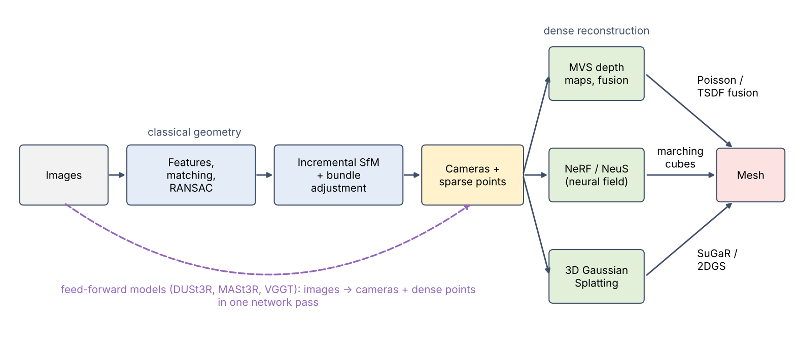
This tutorial assumes you know keypoints and descriptor matching from IP 12 and the basics of deep networks from DLCV 01. The standard textbook for the geometry is Hartley and Zisserman [1].
Related chapters. DLCV 11A treats the dense correspondence problems behind reconstruction — stereo matching, monocular depth and optical flow — in depth, and DLCV 03B uses 3D geometry to detect objects.
What 3D reconstruction is
Plain version. From photos of a static scene, estimate camera poses and a 3D representation of its shape and appearance.
Precise version. We are given images of a static scene. We want camera parameters for each image (defined in the next section) and a scene model such that rendering with camera reproduces . Two variants matter. Geometric reconstruction asks for an accurate surface; it is judged against laser or structured-light scans. Novel-view synthesis asks for realistic images from camera positions that were not photographed; it is judged against held-out photos. NeRF and 3DGS were designed for the second goal, which is why extracting a good surface from them took extra work.
The problem has a built-in limitation: from photos alone, the whole scene can be scaled up or down without changing any image. A toy house photographed from close by and a real house photographed from far away can produce the same pictures. Reconstruction from images is therefore defined only up to scale (and up to the choice of the world coordinate frame) unless something else, such as a known distance or a calibrated stereo rig, fixes it [1].
Seven ways to store a 3D scene
Plain version. Choose the representation for the operation: rendering, measurement, editing or learning. Figure 2 compares common forms on the same scene.
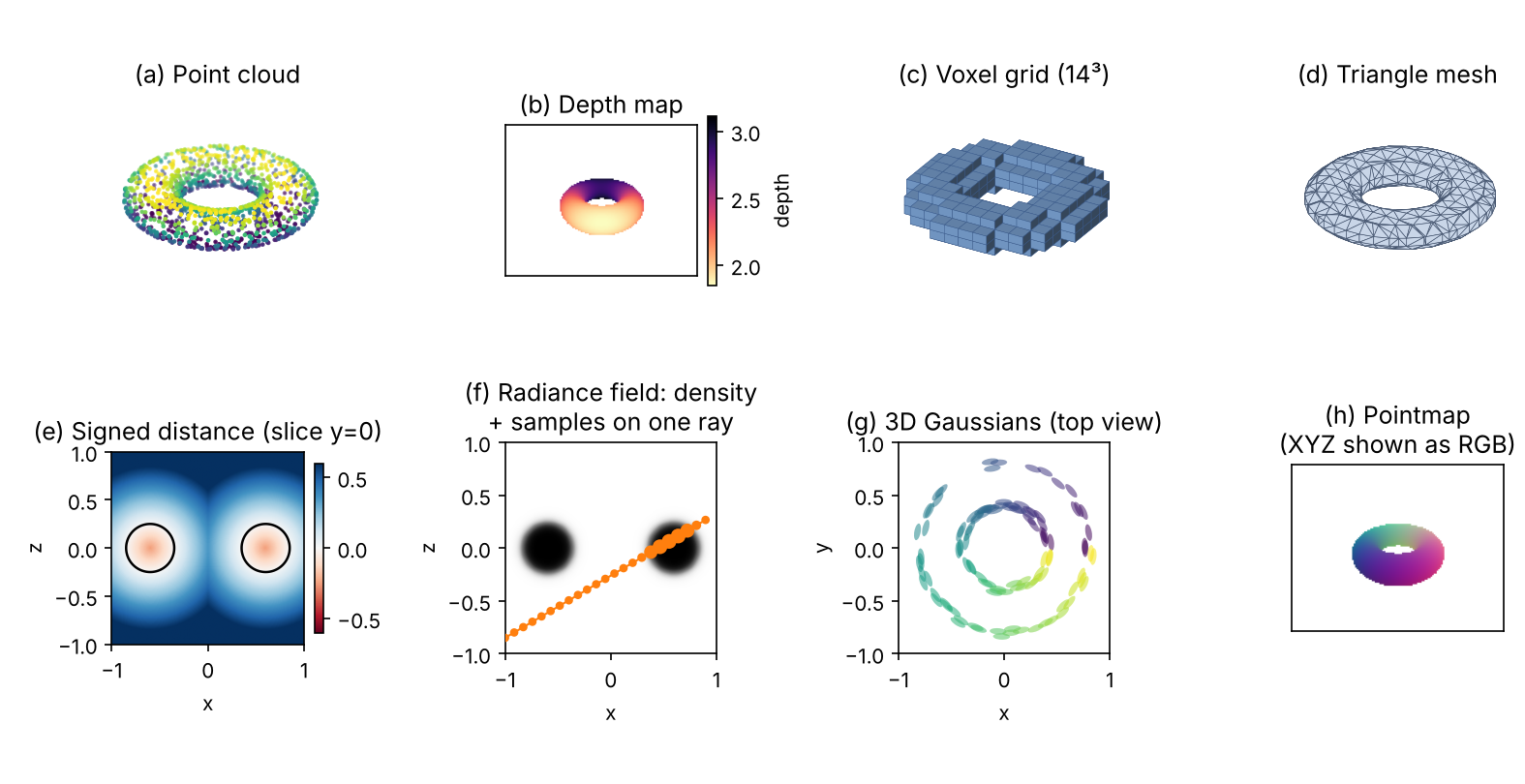
| Representation | What is stored | Strengths | Weaknesses |
|---|---|---|---|
| Point cloud | A list of 3D points, often with colour and normal | Simple; direct output of triangulation and depth sensors | No surface or connectivity; holes; hard to render nicely |
| Depth map | One distance per pixel of one camera | Fits image networks; easy to estimate per view | Covers one viewpoint only; must be fused |
| Voxel grid | A value (occupancy, colour) per cell of a 3D grid | Regular, easy to process with 3D convolutions | Memory grows with the cube of resolution |
| Mesh | Vertices and triangles | Compact, editable, what graphics engines and printers use | Fixed topology; hard to optimize directly from images |
| Signed distance function (SDF) | Distance to the nearest surface, negative inside | Watertight surface as the zero level set; normals from the gradient | Needs a closed surface; must be converted for rendering |
| Radiance field | Density and view-dependent colour at every 3D point | Photorealistic novel views, including thin and fuzzy structures | Slow to render with ray marching; surface is implicit |
| 3D Gaussians | Many small ellipsoids with colour and opacity | Real-time rendering; explicit and editable | Many primitives (memory); surfaces are not well defined |
An SDF can be a stored grid or a function computed by a network: DeepSDF [20] learns a network that outputs signed distance, and Occupancy Networks [21] learn the probability that a point is inside the object. Both are called neural implicit representations, because the surface is given implicitly as a level set of a learned function.
Camera geometry essentials
Plain version. The pinhole model maps a 3D point to image coordinates through camera transformation, projection and perspective division.
The pinhole camera: intrinsics and extrinsics
A camera does two things to a 3D point. It first describes the point relative to itself (how far to the left, up and ahead of the camera it is), then flattens it onto the sensor by dividing by its distance. In symbols, a world point is first moved into the camera’s coordinate frame, then projected:
where (a rotation) and (a translation) are the extrinsics: they say where the camera is and which way it points; is the point in camera coordinates, with the axis along the viewing direction; holds the intrinsics: focal lengths in pixels, the principal point where the optical axis meets the image, and a skew that is zero for real sensors; is the pixel; and equals the depth of the point. Dividing by depth is what makes far things look small. The camera centre in world coordinates is . Combining both steps gives the projection matrix .
Real lenses also bend straight lines (radial distortion); calibration tools estimate extra distortion coefficients and undistort the images first, so the rest of this tutorial assumes an ideal pinhole. The homogeneous coordinates used here, with their trailing 1, are the same as in the homography note of IP 02 (Homography: the projective transform).
Two views: epipolar geometry
Plain version. If you see a point in one photo, you do not know how far away it is, so in 3D it could lie anywhere on a ray. In the second photo, that ray appears as a line. The true match must sit on that line. This turns a 2D search into a 1D search and, in reverse, lets us recover how the two cameras are placed from matched points alone.
Figure 3 (a) shows the geometry. The two camera centres and the 3D point span a plane, the epipolar plane. It cuts each image in an epipolar line. Any point on the same ray of camera 1 has the same image in camera 1, and its image in camera 2 moves along that line.
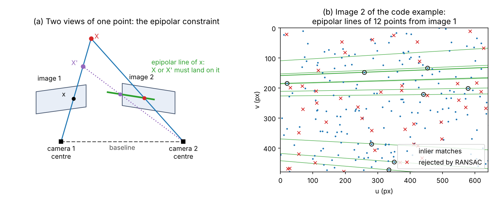
In algebra, let and be the normalized coordinates of a matched pair (pixels with the intrinsics removed). If camera 2 sits at rotation and translation relative to camera 1, every correct match satisfies
where is the essential matrix [7] and is the matrix that computes the cross product with . The equation says that the two viewing rays and the baseline lie in one plane. In pixel coordinates the same constraint reads with the fundamental matrix , where are homogeneous pixel coordinates. is exactly the epipolar line in image 2 drawn in Figure 3 (b).
In plain words: encodes the relative pose of two calibrated cameras, and does the same when the intrinsics are unknown. has five degrees of freedom: three for the rotation and two for the direction of the translation, whose length is lost to the scale ambiguity. Five matches therefore suffice, the minimal case solved by Nistér’s five-point algorithm [9]. With eight or more matches the constraint is linear in the nine entries of or : the eight-point algorithm [7], [8] stacks one equation per match and takes the null vector with the singular value decomposition.
Optional: The normalized eight-point algorithm (in the Supplementary notes). Why the pixel coordinates must be rescaled first, the rank-2 step, and a test of both versions.
Once is known, it can be factored into and the direction of . The factorization gives four candidate poses; only one places the points in front of both cameras, which is called the cheirality (or chirality) check [1].
Triangulation
Plain version. With both cameras known, a matched pair gives two rays. Where they (almost) cross is the 3D point. Noise means they never meet exactly, so we pick the point that best explains both observations.
The simplest method is linear. Each image gives two linear equations in the unknown point (the pinhole equation with the unknown depth eliminated), and the four equations are solved, like the eight-point system, as the null vector of a small matrix with the SVD [1]. The quality of a triangulated point is judged by its reprojection error: project it back into each image and measure the pixel distance to the observed point.
Optional: Linear triangulation (DLT) (in the Supplementary notes). The four equations written out, why the linear answer is not the optimal one, and a test of how the baseline controls the error.
Accuracy depends strongly on the angle between the two rays. For two parallel cameras with focal length and baseline , a point at depth shifts by the disparity pixels between the images, so a small disparity error gives a depth error . Depth error grows with the square of distance and shrinks with a wider baseline; Exercise 1 puts numbers on this.
Code: relative pose and triangulation
The snippet builds a synthetic scene, projects it into two cameras with 0.5-pixel noise, replaces 15% of the matches by random wrong ones, and then recovers the relative pose with OpenCV. cv2.findEssentialMat runs RANSAC around the five-point solver (its documentation names Nistér’s algorithm [9]); cv2.recoverPose performs the cheirality check. RANSAC’s answer comes from a minimal sample, so we refit linearly on all inliers, the “refit on the consensus set” step described in the RANSAC note of IP 12 (RANSAC: fitting a model despite outliers).
Code · Python · 56 lines
import numpy as np
import cv2

rng = np.random.default_rng(0)
K = np.array([[800.0, 0, 320], [0, 800.0, 240], [0, 0, 1]])   # focal length 800 px, principal point (320, 240)

def look_at(C, target):
    """Rotation of a camera at centre C that looks at target (rows: camera x, y, z axes)."""
    z = (target - C) / np.linalg.norm(target - C)
    x = np.cross([0.0, 1.0, 0.0], z); x /= np.linalg.norm(x)
    return np.stack([x, np.cross(z, x), z])

def project(K, R, t, X):
    """Pinhole projection of world points X (N, 3) to pixels (N, 2)."""
    x = (X @ R.T + t) @ K.T           # world -> camera -> homogeneous pixels
    return x[:, :2] / x[:, 2:]        # divide by depth

def linear_E(x1, x2, K):
    """Least-squares E from many matches: each match gives one linear equation in E's 9 entries."""
    Ki = np.linalg.inv(K)
    a = np.c_[x1, np.ones(len(x1))] @ Ki.T               # normalized camera coordinates
    b = np.c_[x2, np.ones(len(x2))] @ Ki.T
    A = np.einsum('ni,nj->nij', b, a).reshape(-1, 9)      # row n encodes b_n^T E a_n = 0
    E = np.linalg.svd(A)[2][-1].reshape(3, 3)             # best null vector of A
    U, _, Vt = np.linalg.svd(E)
    return U @ np.diag([1.0, 1.0, 0.0]) @ Vt              # nearest valid essential matrix

X = rng.uniform([-3, -2, 4], [3, 2, 8], size=(300, 3))           # 300 scene points
C2 = np.array([2.0, 0.0, 0.0])                                    # camera 2 centre: 2 units to the right
R2 = look_at(C2, np.array([0.0, 0.0, 6.0])); t2 = -R2 @ C2        # camera 1 is the world frame
x1 = project(K, np.eye(3), np.zeros(3), X) + rng.normal(0, 0.5, (300, 2))   # 0.5 px noise
x2 = project(K, R2, t2, X) + rng.normal(0, 0.5, (300, 2))
x2[:45] = rng.uniform([0, 0], [640, 480], (45, 2))                # 45 wrong matches (15 %)

def pose_errors(R, t):
    rot = np.degrees(np.arccos(np.clip((np.trace(R.T @ R2) - 1) / 2, -1, 1)))
    return rot, np.degrees(np.arccos(t.ravel() @ t2 / np.linalg.norm(t2)))

E, mask = cv2.findEssentialMat(x1, x2, K, method=cv2.RANSAC, prob=0.999, threshold=1.5)
_, R, t, mask = cv2.recoverPose(E, x1, x2, K, mask=mask)
inl = mask.ravel() > 0
print(f"inliers kept: {inl.sum()} of 300 | wrong matches rejected: {(~inl[:45]).sum()} of 45")
print("RANSAC estimate      : rotation error %.2f deg, translation direction error %.2f deg" % pose_errors(R, t))
_, R, t, _ = cv2.recoverPose(linear_E(x1[inl], x2[inl], K), x1[inl], x2[inl], K)
print("refit on all inliers : rotation error %.2f deg, translation direction error %.2f deg" % pose_errors(R, t))
print(f"length of estimated t: {np.linalg.norm(t):.2f} (true baseline {np.linalg.norm(C2):.2f})")

P1 = K @ np.hstack([np.eye(3), np.zeros((3, 1))])     # P1 = K [I | 0]
P2 = K @ np.hstack([R, t])                            # P2 = K [R | t]
Xh = cv2.triangulatePoints(P1, P2, x1[inl].T, x2[inl].T)
Xe = (Xh[:3] / Xh[3]).T                               # homogeneous -> Euclidean
res = np.r_[np.linalg.norm(project(K, np.eye(3), np.zeros(3), Xe) - x1[inl], axis=1),
            np.linalg.norm(project(K, R, t.ravel(), Xe) - x2[inl], axis=1)]
print(f"reprojection error: RMS {np.sqrt(np.mean(res ** 2)):.2f} px")
rel = np.linalg.norm(2.0 * Xe - X[inl], axis=1) / np.linalg.norm(X[inl], axis=1)   # scale fixed by the true baseline
print(f"3D error after fixing the scale: median {100 * np.median(rel):.2f} % of the distance")
Output
inliers kept: 250 of 300 | wrong matches rejected: 44 of 45
RANSAC estimate      : rotation error 0.30 deg, translation direction error 0.42 deg
refit on all inliers : rotation error 0.07 deg, translation direction error 0.46 deg
length of estimated t: 1.00 (true baseline 2.00)
reprojection error: RMS 0.40 px
3D error after fixing the scale: median 0.31 % of the distance
These numbers are from this synthetic run only. RANSAC rejects 44 of the 45 wrong matches. Refitting on all inliers reduces the rotation error from 0.30° to 0.07°; the translation direction stays within half a degree either way. The estimated translation has length exactly 1: OpenCV returns only its direction, because the images cannot tell the true baseline of 2. Once the scale is supplied from outside, the triangulated points are within about 0.3% of their true distance. The reprojection error of 0.40 px is below the 0.5 px noise level, as expected when the points are fitted to their own observations.
Structure from motion
Plain version. Structure from motion (SfM) does the two-view trick for hundreds of photos at once: it finds matching points across all of them, places the cameras one by one, triangulates the points, and keeps polishing everything so that all 3D points project onto their observed pixels.
Features, matching and geometric verification
First, SfM must know which pixels in different photos show the same physical point. It starts with local features. Each image yields keypoints with descriptors, such as SIFT [11] (IP 12), and descriptors are matched between image pairs (IP 12, Matching). Many matches are wrong, so each pair is geometrically verified: RANSAC [10] fits a fundamental matrix (or an essential matrix or a homography) and keeps the pair only if enough matches agree [2]. The verified pairs form a scene graph: images are nodes, and an edge means “these two images see the same points”.
Incremental reconstruction
COLMAP’s paper describes the standard incremental pipeline [2], which grew out of earlier systems for Internet photo collections such as Photo Tourism [12]:
- Initialize with a carefully chosen pair of images that share many matches and have a wide baseline; estimate their relative pose and triangulate the shared points.
- Register a new image by solving the Perspective-n-Point (PnP) problem: find the camera pose from matches between its keypoints and already triangulated 3D points, inside RANSAC.
- Triangulate new points seen by the new image and at least one registered image.
- Bundle adjust (below) to refine all cameras and points together, then filter points with large reprojection error.
- Repeat from step 2 until no more images can be registered.
The COLMAP paper improves each of these steps, including how the next image is chosen and how points are triangulated. Its central lesson is in step 4: registration and triangulation must be interleaved with repeated bundle adjustment, re-triangulation and outlier filtering, because without that refinement small errors accumulate as images are added and the reconstruction drifts [2].
Bundle adjustment
Plain version. Bundle adjustment (BA) is the final polish: move every camera and every 3D point a little until all the “bundles” of rays line up with the pixels where the points were actually seen.
BA solves the nonlinear least-squares problem
where are the parameters of camera (pose, and intrinsics if unknown), are the 3D points, is the set of observations (point seen in image ), is the observed pixel, is the pinhole projection, and is a robust loss that down-weights outliers [2], [13]. The standard solver is Levenberg–Marquardt, a damped Gauss–Newton method. It is fast because each residual depends on only one camera and one point, so the Jacobian is almost all zeros [2], [13]. BA cannot fix the global scale and coordinate frame, and it finds only a local minimum, so it needs the good starting point that the incremental steps provide.
Optional: Bundle adjustment in code (in the Supplementary notes). A complete small BA with scipy.optimize.least_squares, its sparsity pattern, and the gauge problem.
COLMAP in practice
COLMAP is the open-source SfM and MVS pipeline released with [2] and [3], with a graphical and a command-line interface [4]. It outputs the camera intrinsics and poses plus a sparse point cloud, the standard input of the dense methods below: the NeRF paper takes the poses of its real scenes from COLMAP [5], and 3DGS initializes its Gaussians from the SfM points [6]. Every later stage inherits the errors made here (see Pose errors under failure modes).
Multi-view stereo
Plain version. SfM gives cameras and a sparse set of points. Multi-view stereo (MVS) fills in the rest: for every pixel of a reference image it searches, along the epipolar line in the other images, for the depth at which all views agree on what the surface looks like.
Photo-consistency and plane sweep
The core test is photo-consistency: if a pixel’s surface point is at depth , then the small patch around it should look the same in every image that sees that point. A depth hypothesis is scored by a matching cost such as the sum of squared differences (SSD) or normalized cross-correlation between patches.
The plane sweep algorithm [14] tests many depths efficiently. Sweep a plane, parallel to the reference image, through a range of depths . For each depth, warp every source image onto the reference view as if the whole scene lay on that plane; the warp for one plane is a homography. Compute the cost per pixel, stack the costs into a cost volume of size , and choose for each pixel the depth with the lowest cost:
where is the source image warped by the plane at depth and is a small window around the pixel. For two parallel cameras (a rectified pair), the plane homography reduces to a horizontal shift by the disparity , which keeps the code short.
Optional: The plane-induced homography (in the Supplementary notes). The warp for general camera poses and tilted planes.
Code · Python · 36 lines
import numpy as np
from scipy import ndimage as ndi

rng = np.random.default_rng(0)
H, W, f, B = 120, 160, 150.0, 0.5                     # image size, focal length (px), baseline
tex = ndi.gaussian_filter(rng.random((400, 400)), 1.5)   # random texture painted on the world
tex = (tex - tex.min()) / np.ptp(tex)

def render(cx):
    """Ray-cast a camera at (cx, 0, 0) looking down +Z: a square at Z=5 in front of a wall at Z=8."""
    v, u = np.mgrid[0:H, 0:W].astype(float)
    dx, dy = (u - W / 2) / f, (v - H / 2) / f          # ray direction (dx, dy, 1)
    Xs, Ys = cx + 5 * dx, 5 * dy                        # hit point on the plane Z = 5
    front = (np.abs(Xs) < 1) & (np.abs(Ys) < 1)         # inside the square?
    Z = np.where(front, 5.0, 8.0)
    X, Y = cx + Z * dx, Z * dy
    img = ndi.map_coordinates(tex, [200 + 40 * Y + 100 * front, 200 + 40 * X], order=1)
    img[~front & (X > 1.5) & (Y < -0.5)] = 0.5          # a textureless patch on the wall
    return img, Z

ref, Z_true = render(0.0)                              # reference camera
src, _ = render(B)                                     # source camera, B to the right

depths = 1 / np.linspace(1 / 10, 1 / 3.5, 80)          # depth hypotheses, uniform in 1/Z
cost = np.empty((len(depths), H, W))
for k, Z in enumerate(depths):
    d = f * B / Z                                      # the plane Z induces a horizontal shift d
    warped = ndi.shift(src, (0, d), order=1, mode='nearest')   # src pixel u - d lands on u
    cost[k] = ndi.uniform_filter((ref - warped) ** 2, 7)       # windowed SSD photo-consistency
Z_est = depths[cost.argmin(0)]                         # winner-take-all depth per pixel

ok = np.abs(Z_est - Z_true) / Z_true < 0.05
flat = (Z_true == 8) & (ref == 0.5)
inner = np.zeros_like(ok); inner[8:-8, 20:-8] = True    # ignore borders the source camera cannot see
print(f"pixels within 5% of the true depth: {100 * ok[inner & ~flat].mean():.1f}% (textured), "
      f"{100 * ok[inner & flat].mean():.1f}% (textureless patch)")
Output
pixels within 5% of the true depth: 95.3% (textured), 14.8% (textureless patch)On textured surfaces 95.3% of the evaluated pixels get a depth within 5% of the truth in this synthetic run. In the textureless patch only 14.8% do, because every depth hypothesis matches a flat grey patch equally well. Figure 4 (d) shows this directly: the cost curve of the textured pixel has one sharp minimum at the true depth; the curve of the textureless pixel is flat. The remaining errors on textured surfaces sit at the left border (seen by one camera only) and next to the square, where part of the background is hidden from the second camera (occlusion).
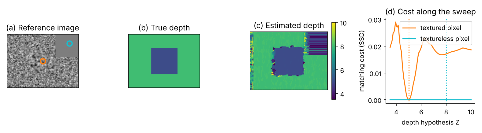
From depth maps to one model
A depth map per image is not yet one model. Depth-map fusion merges them. The volumetric method of Curless and Levoy [15] stores, in a voxel grid, a running weighted average of the signed distance to the surface measured by each depth map:
where is the signed distance from voxel to the surface seen in depth map along the viewing ray, is its confidence weight, and , are the accumulated distance and weight after maps. The surface is the zero level set of , extracted by marching cubes (below). In practice the distances are truncated near the surface, hence the name TSDF (truncated signed distance function) fusion. COLMAP’s MVS [3] instead estimates a depth and a normal per pixel with per-pixel view selection and a multi-view geometric consistency check, then fuses the consistent depths into a dense point cloud.
Learning-based MVS
Plain version. The hand-made parts of MVS, the patch cost and the rules that clean up the cost volume, can be learned from data.
MVSNet [16] keeps the plane-sweep structure but makes every step differentiable. A shared CNN extracts features from all images, and the features of each source view are warped onto fronto-parallel planes of the reference camera (differentiable homography warping). A variance-based cost merges any number of views into one cost volume: low variance means the views agree. A 3D CNN regularizes the volume, a softmax along the depth axis gives a probability per depth, and the expected depth under that distribution (the “soft argmin”) is a continuous output that can be trained with a regression loss [16]. MVSNet was trained on DTU [37] and evaluated on Tanks and Temples [38] without fine-tuning [16]. Its authors motivate learning with the low-textured, specular and reflective regions where hand-made costs fail [16].
Neural radiance fields (NeRF)
Plain version. NeRF stores a scene as a small neural network that answers one question for any point in space and any viewing direction: “how much stuff is here, and what colour does it send toward me?” To make an image, it shoots a ray through each pixel, asks the network at many points along the ray, and blends the answers. Training adjusts the network until the rendered images match the photos.
The scene as a function
NeRF [5] is a multilayer perceptron , where is a position, a viewing direction, the volume density at and the RGB colour emitted toward . The network is built so that density depends on position only, while colour also depends on direction, which lets NeRF reproduce shiny highlights that change with the viewpoint [5]. One network represents one scene; there is no training set of many scenes.
Optional: NeRF (Mildenhall et al., 2020) (in the Paper guides). What the paper set out to solve, what its tables and ablations show, and what it does not claim.
Volume rendering along a ray
Plain version. Picture the ray as passing through fog of varying thickness. Each bit of fog both glows with its own colour and blocks the light from behind it. The pixel colour is the sum of all the glows, each dimmed by the fog in front of it.
A camera ray is with origin (the camera centre), direction and distance between near and far bounds and . Following classical volume rendering [17], the expected colour is
where is the transmittance, the probability that the ray travels from to without being stopped [5]. NeRF evaluates it with samples along the ray:
where are the network outputs at sample , is the spacing, is the opacity of segment , is the light that survives the segments before it, and is the weight of sample in the pixel. This is exactly front-to-back alpha compositing of semi-transparent layers [5]. The sum of the weights, , is the pixel’s total opacity, and is an estimate of depth. Every step is differentiable, so the photo error can be pushed back into the network weights.
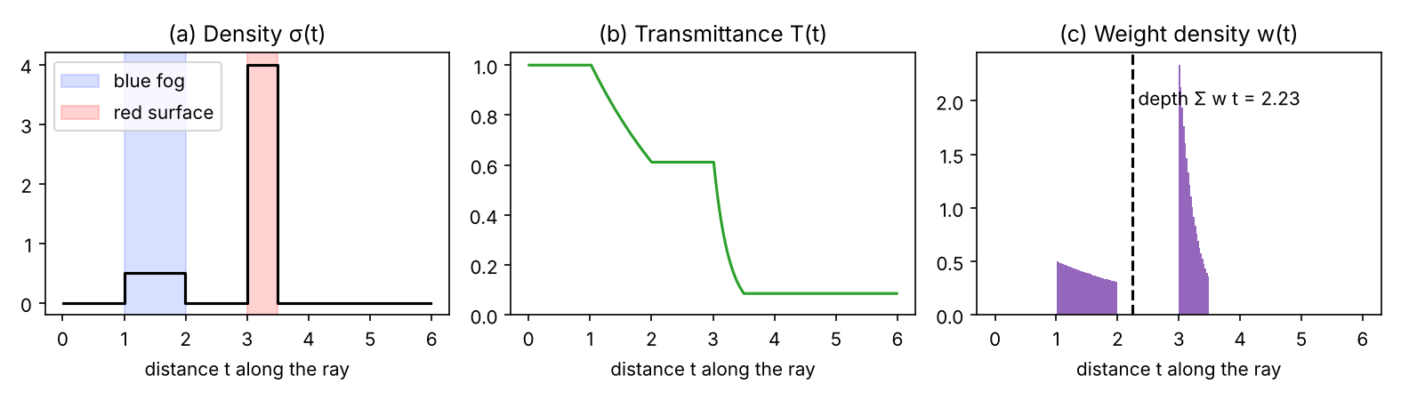
The snippet checks the quadrature against an exact answer. The ray crosses blue fog, then a red surface layer, then reaches a white background; for piecewise-constant density the integrals have closed forms.
Code · Python · 40 lines
import numpy as np

# One ray from t = 0 to t = 6: blue fog on [1, 2] (density 0.5), a red surface on [3, 3.5] (density 4),
# white background behind everything.
slabs = [(1.0, 2.0, 0.5, np.array([0.2, 0.4, 1.0])),
         (3.0, 3.5, 4.0, np.array([1.0, 0.1, 0.1]))]
bg = np.ones(3)

def field(t):
    """Density sigma(t) and colour c(t) at sample positions t."""
    sigma, c = np.zeros_like(t), np.zeros(t.shape + (3,))
    for a, b, s, col in slabs:
        inside = (t >= a) & (t < b)
        sigma[inside], c[inside] = s, col
    return sigma, c

def render(n):
    """NeRF quadrature: alpha_i = 1 - exp(-sigma_i delta_i), T_i = prod_{j<i} (1 - alpha_j), w_i = T_i alpha_i."""
    edges = np.linspace(0, 6, n + 1)
    t, delta = (edges[:-1] + edges[1:]) / 2, np.diff(edges)
    sigma, c = field(t)
    alpha = 1 - np.exp(-sigma * delta)
    T = np.concatenate([[1.0], np.cumprod(1 - alpha)[:-1]])
    w = T * alpha
    T_end = T[-1] * (1 - alpha[-1])                   # light that reaches the background
    return w @ c + T_end * bg, w.sum(), w @ t

# Analytic answer for piecewise-constant density (exact integrals of the volume rendering equation)
C, acc, depth, T0 = np.zeros(3), 0.0, 0.0, 1.0
for a, b, s, col in slabs:
    L = b - a
    absorbed = T0 * (1 - np.exp(-s * L))
    C, acc = C + absorbed * col, acc + absorbed
    depth += T0 * (a * (1 - np.exp(-s * L)) + (1 - np.exp(-s * L)) / s - L * np.exp(-s * L))
    T0 *= np.exp(-s * L)
C += T0 * bg
print(f"analytic : colour {np.round(C, 4)}, opacity {acc:.4f}, depth {depth:.4f}")
for n in [16, 64, 256, 1024]:
    Cq, accq, dq = render(n)
    print(f"N = {n:4d} : colour {np.round(Cq, 4)}, opacity {accq:.4f}, depth {dq:.4f}")
Output
analytic : colour [0.6852 0.2919 0.528 ], opacity 0.9179, depth 2.2373
N =   16 : colour [0.7498 0.3318 0.5195], opacity 0.8466, depth 2.1655
N =   64 : colour [0.7006 0.2986 0.5232], opacity 0.9040, depth 2.2263
N =  256 : colour [0.689  0.2934 0.5267], opacity 0.9146, depth 2.2348
N = 1024 : colour [0.6862 0.2923 0.5277], opacity 0.9171, depth 2.2367
The quadrature converges to the analytic colour, opacity and depth as the number of samples grows. With 16 samples it is visibly off, because the thin surface layer falls into one or two coarse bins. This is why NeRF does not sample uniformly: a coarse network with 64 samples per ray first finds where the weights are large, and a fine network adds 128 samples concentrated there (hierarchical sampling) [5]. Note also the depth: 2.24 (2.23 with the 256 samples of Figure 5), between the fog and the surface, where no surface exists. Semi-transparent “fog” in the wrong place is the origin of the floater artifacts discussed under failure modes. Figure 5 plots the density, transmittance and weights for this ray.
Positional encoding
Plain version. A plain MLP fed with raw learns smooth, blurry functions. Feeding it sines and cosines of the coordinates at many frequencies lets it represent sharp edges and fine texture.
NeRF maps each coordinate (normalized to ) to
where is the number of frequency bands: for position and for direction [5]. Without the encoding, the paper’s results lose their fine detail [5]. Tancik et al. [18] explained why: coordinate MLPs are biased toward low frequencies (a spectral bias), and a Fourier feature mapping of the input removes this bias. The sinusoids resemble the positional information of Transformers (ML 05), but here they encode continuous coordinates rather than token positions.
Training, and why it is slow
Training needs posed images and nothing else. Each step samples a batch of pixels (rays) from the training images, renders them with the coarse and fine networks, and minimizes the squared colour error [5]. The cost is the problem. Every pixel needs hundreds of network evaluations, and a scene needs a few hundred thousand steps. The paper reports 100–300k iterations, about 1–2 days on one NVIDIA V100 GPU, per scene [5]. Rendering is slow for the same reason: the paper uses 256 network queries per ray, between 150 and 200 million per image, and reports about 30 seconds per frame on a V100 [5].
Making it fast: hash grids
Plain version. Instead of asking one big network to remember everything, store learned features in lookup tables at several resolutions, and use a tiny network to decode them. Looking up a table is far cheaper than running many network layers.
Instant-NGP [19] replaces the frequency encoding with a multiresolution hash encoding. Space is covered by grids, from coarse to fine. Each grid stores trainable feature vectors at its corners, but in a table of fixed size ; on fine grids, where there are far more corners than table entries, a hash function decides which entry a corner uses, so several corners share one entry. To encode a point, the features of the corners around it are interpolated on every level, concatenated and passed to a small MLP. The paper does not resolve the shared entries explicitly; it relies on the coarse levels and the MLP to sort them out [19]. The authors report training of high-quality results “in a matter of seconds” and rendering in tens of milliseconds at 1920 × 1080 on one GPU [19]. Grid-based encodings of this kind are now common in fast NeRF variants.
Optional: The multiresolution hash encoding (in the Supplementary notes). The level resolutions, the hash function, the parameter count, and a worked example.
Neural implicit surfaces: NeuS
Plain version. NeRF’s density does not have to form a clean surface: it can be a cloud. If you want a surface, let the network output a signed distance instead, and convert distance to opacity in a way that makes the rendered weight peak exactly on the surface.
NeuS [22] represents the scene as an SDF network whose zero level set is the surface. It converts the SDF into opacity through the sigmoid , where is a learned sharpness that grows during training. The authors show that the obvious choice, using the logistic density directly as the volume density, gives weights that peak before the surface (the bias), and they derive an opacity that is unbiased to first order and still handles occlusion [22]. In discrete form,
where is the -th sample on the ray; the weights then follow the same compositing formula as NeRF. An Eikonal term keeps a valid distance function [22]. Because the surface is a level set, a mesh follows directly from marching cubes. NeuS reconstructs objects without foreground masks, and it was evaluated on DTU [37] among other data [22].
Optional: Why NeuS weights peak on the surface (in the Supplementary notes). The bias of the naive density, measured on one ray.
3D Gaussian Splatting
Plain version. Instead of a network you must query along every ray, 3DGS represents the scene with millions of small, coloured, semi-transparent ellipsoids, like a cloud of soft paint drops. To make an image it projects each drop onto the screen as a soft ellipse and stacks them from front to back. No ray marching, no network: just sorting and blending, which a GPU does very fast.
The Gaussian primitive
Each blob is a 3D bell curve: dense at its centre, fading smoothly outward, and stretched more in some directions than in others. Precisely, each primitive [6] has a centre , a covariance that sets its size and orientation, an opacity and a colour stored as spherical-harmonic coefficients (a small set of smooth functions on the sphere, so the colour can change with the viewing direction). Its footprint in space is
where holds the three axis lengths and is a rotation stored as a unit quaternion [6]. The factorization guarantees that stays a valid (positive semi-definite) covariance during gradient descent, which optimizing the six entries of directly would not [6].
Projection to the image
Plain version. A 3D ellipsoid seen through a camera looks like a 2D ellipse. 3DGS computes that ellipse with a local linear approximation of the camera projection, which is accurate for small Gaussians.
Following EWA splatting [23], the 2D covariance of the projected Gaussian is
where is the rotation part of the world-to-camera transform, is the Jacobian of the perspective projection evaluated at the Gaussian’s centre, and keeping only the top-left block of gives the image-space ellipse [6], [23]. The projected centre is simply the pinhole projection of .
Optional: Projecting a 3D Gaussian: the local affine approximation (in the Supplementary notes). The Jacobian written out, and when the approximation breaks.
Alpha compositing and real-time rendering
The pixel colour uses the same compositing rule as NeRF, but over the Gaussians that cover the pixel, sorted by depth:
where is the pixel position, and are the projected centre and covariance of Gaussian , and its view-dependent colour. Why is it fast? The renderer [6] splits the screen into -pixel tiles, assigns each visible Gaussian to the tiles it touches, sorts all (tile, depth) keys once with a GPU radix sort, and then blends each tile’s list front to back in parallel, stopping a pixel once it is nearly opaque. There is no network to evaluate and no empty space to sample. The paper reports real-time (at least 30 frames per second) novel-view synthesis at 1080p with quality comparable to the best NeRF variant of the time [6].
Optional: 3D Gaussian Splatting (Kerbl et al., 2023) (in the Paper guides). How to separate the representation from the engineering when you read the paper, and its stated limitations.
Optimization and adaptive density control
Plain version. Training starts from the sparse SfM points, one Gaussian per point, and then grows and prunes the set: where detail is missing it adds Gaussians, where one big Gaussian covers too much it splits it, and invisible ones are removed.
All parameters are optimized by gradient descent on the loss between rendered and real images, with [6]. Every 100 iterations the method densifies Gaussians whose view-space position gradient is large, a sign that the region is not yet well explained [6]:
- a small Gaussian in an under-reconstructed region is cloned (copied and moved along the gradient);
- a large Gaussian in a region of high variance is split into two smaller ones, with scales divided by 1.6;
- Gaussians with opacity below a threshold are pruned; in addition, all opacities are reset close to zero every 3000 iterations, which limits the growth of Gaussians caused by floaters close to the input cameras [6].
Code: a toy 2D splatting fit
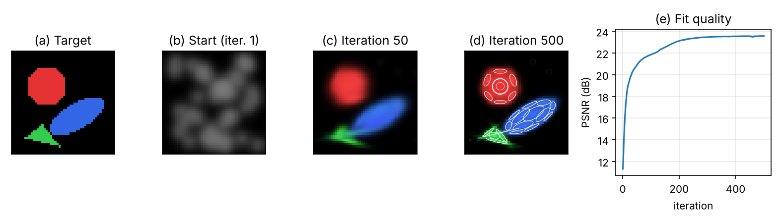
The snippet fits 40 two-dimensional Gaussians to a 48 × 48 image with the Adam optimizer [49], using exactly the compositing rule above (with a fixed depth order and no densification). The backward pass is written out by hand with the chain rule (the 3DGS paper likewise derives its gradients explicitly instead of relying on automatic differentiation [6]); the gradient was checked against finite differences while writing this tutorial.
Code · Python · 64 lines
import numpy as np
from skimage.draw import disk, polygon, ellipse

# Target: a small synthetic RGB image (48 x 48) on a black background
H = W = 48
target = np.zeros((H, W, 3))
target[disk((16, 16), 9)] = [0.9, 0.2, 0.2]
target[ellipse(30, 30, 6, 14, rotation=np.deg2rad(30))] = [0.2, 0.4, 0.9]
target[polygon([40, 44, 34], [6, 22, 14])] = [0.2, 0.8, 0.3]
ys, xs = np.mgrid[0:H, 0:W].astype(float)

def sig(z):
    return 1 / (1 + np.exp(-z))

def render(p, target=None):
    """Front-to-back alpha compositing of K 2D Gaussians (index order = depth order).
    p: mu (K,2), log_s (K,2), theta (K,), op (K,) opacity logits, col (K,3) colour logits."""
    c, s, th = sig(p['col']), np.exp(p['log_s']), p['theta']
    dx = xs[None] - p['mu'][:, 0, None, None]; dy = ys[None] - p['mu'][:, 1, None, None]
    ct, st = np.cos(th)[:, None, None], np.sin(th)[:, None, None]
    u1, u2 = ct * dx + st * dy, -st * dx + ct * dy                   # offsets in the Gaussian's own axes
    sx2, sy2 = (s[:, 0] ** 2)[:, None, None], (s[:, 1] ** 2)[:, None, None]
    g = np.exp(-0.5 * (u1 ** 2 / sx2 + u2 ** 2 / sy2))               # Gaussian footprint
    o = sig(p['op'])[:, None, None]
    a = np.minimum(o * g, 0.99)                                       # alpha of each Gaussian at each pixel
    T = np.cumprod(np.concatenate([np.ones((1, H, W)), 1 - a[:-1]]), axis=0)   # transmittance in front
    w = a * T                                                          # compositing weights
    img = np.einsum('khw,kc->hwc', w, c)                              # black background adds nothing
    if target is None:
        return img
    # backward pass for the loss L = mean squared error (the chain rule written out by hand)
    G = 2 * (img - target) / target.size                               # dL/dimg, shape (H, W, 3)
    contrib = w[..., None] * c[:, None, None, :]                       # (K, H, W, 3)
    behind = np.cumsum(contrib[::-1], axis=0)[::-1] - contrib          # colour from Gaussians behind k
    dC_da = T[..., None] * c[:, None, None, :] - behind / (1 - a[..., None])
    da = np.einsum('khwc,hwc->khw', dC_da, G) * (o * g < 0.99)
    dq = da * o * g * -0.5                                             # through g = exp(-q / 2)
    grads = {
        'col': np.einsum('khw,hwc->kc', w, G) * c * (1 - c),
        'op': (da * g).sum((1, 2)) * sig(p['op']) * (1 - sig(p['op'])),
        'log_s': np.stack([(dq * -2 * u1 ** 2 / sx2).sum((1, 2)), (dq * -2 * u2 ** 2 / sy2).sum((1, 2))], 1),
        'theta': (dq * 2 * u1 * u2 * (1 / sx2 - 1 / sy2)).sum((1, 2)),
        'mu': -np.stack([(dq * (2 * u1 * ct / sx2 - 2 * u2 * st / sy2)).sum((1, 2)),
                         (dq * (2 * u1 * st / sx2 + 2 * u2 * ct / sy2)).sum((1, 2))], 1),
    }
    return img, grads

rng = np.random.default_rng(0)
K = 40
p = {'mu': rng.uniform(4, 44, (K, 2)), 'log_s': np.full((K, 2), np.log(3.0)), 'theta': rng.uniform(0, np.pi, K),
     'op': np.zeros(K), 'col': np.zeros((K, 3))}
lr = {'mu': 0.5, 'log_s': 0.05, 'theta': 0.05, 'op': 0.1, 'col': 0.1}
m = {k: np.zeros_like(v) for k, v in p.items()}; v2 = {k: np.zeros_like(v) for k, v in p.items()}

def psnr(img):
    return 10 * np.log10(1 / np.mean((img - target) ** 2))

for it in range(1, 501):
    img, gr = render(p, target)
    for k in p:                                                        # Adam update
        m[k] = 0.9 * m[k] + 0.1 * gr[k]; v2[k] = 0.999 * v2[k] + 0.001 * gr[k] ** 2
        p[k] -= lr[k] * (m[k] / (1 - 0.9 ** it)) / (np.sqrt(v2[k] / (1 - 0.999 ** it)) + 1e-8)
    if it in (1, 50, 100, 200, 500):
        print(f"iteration {it:3d}: PSNR {psnr(img):.2f} dB")
Output
iteration   1: PSNR 11.32 dB
iteration  50: PSNR 20.88 dB
iteration 100: PSNR 21.85 dB
iteration 200: PSNR 23.12 dB
iteration 500: PSNR 23.57 dB
PSNR (defined in DLCV 09) rises quickly and then levels off near 23.6 dB in this run. The plateau is the point of the exercise: with a fixed number of soft blobs, sharp corners and the thin tip of the triangle cannot be fitted, and blobs that started in the wrong place stay there. That is exactly what adaptive density control fixes, and Exercise 4 asks you to add it. Figure 6 shows the fit and the final ellipses.
Getting meshes
Plain version. Graphics engines, physics simulators and 3D printers want triangles. Every representation above needs a conversion step to produce them, and the conversion can add its own errors.
Marching cubes
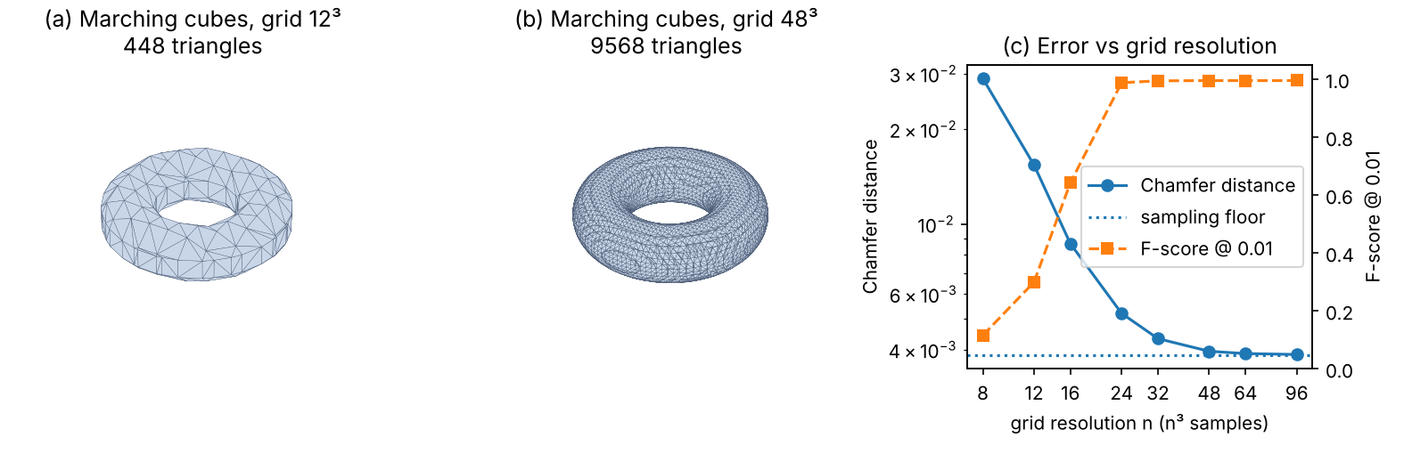
Marching cubes [24] turns a sampled scalar field (an SDF, an occupancy or a fused TSDF) into a triangle mesh of one level set. It visits each cube of eight neighbouring grid samples, looks at which corners are inside and which are outside, places vertices on the cube edges where the sign changes (by linear interpolation of the field values), and connects them with triangles from a lookup table. scikit-image provides an implementation [46]. The snippet extracts the zero level set of an exact torus SDF at several grid resolutions and measures the result with the geometric metrics defined in the evaluation section below.
Code · Python · 46 lines
import numpy as np
from scipy.spatial import cKDTree
from skimage.measure import marching_cubes

R, r = 0.6, 0.25                                       # torus: ring radius R, tube radius r

def sdf_torus(x, y, z):
    """Exact signed distance to the torus (negative inside)."""
    return np.hypot(np.hypot(x, y) - R, z) - r

def sample_mesh(verts, faces, n, rng):
    """n points spread uniformly over the area of a triangle mesh."""
    tri = verts[faces]
    area = 0.5 * np.linalg.norm(np.cross(tri[:, 1] - tri[:, 0], tri[:, 2] - tri[:, 0]), axis=1)
    k = rng.choice(len(faces), n, p=area / area.sum())
    a, b = rng.random((2, n, 1))
    flip = a + b > 1; a[flip], b[flip] = 1 - a[flip], 1 - b[flip]
    return tri[k, 0] + a * (tri[k, 1] - tri[k, 0]) + b * (tri[k, 2] - tri[k, 0])

def sample_torus(n, rng):
    """n points uniform over the true torus surface (rejection sampling on the area element)."""
    u, v = rng.uniform(0, 2 * np.pi, (2, 3 * n))
    ok = rng.random(3 * n) * (R + r) < R + r * np.cos(v)   # keep with probability proportional to R + r cos v
    u, v = u[ok][:n], v[ok][:n]
    return np.c_[(R + r * np.cos(v)) * np.cos(u), (R + r * np.cos(v)) * np.sin(u), r * np.sin(v)]

def geometry_metrics(P, G, tau):
    """Accuracy, completeness, Chamfer (their mean) and F-score at threshold tau."""
    d_pg = cKDTree(G).query(P)[0]                      # each reconstructed point -> nearest true point
    d_gp = cKDTree(P).query(G)[0]                      # each true point -> nearest reconstructed point
    prec, rec = (d_pg < tau).mean(), (d_gp < tau).mean()
    return d_pg.mean(), d_gp.mean(), (d_pg.mean() + d_gp.mean()) / 2, 2 * prec * rec / (prec + rec)

rng = np.random.default_rng(0)
G = sample_torus(100_000, rng)
acc, comp, cd, fs = geometry_metrics(sample_torus(100_000, rng), G, tau=0.01)
print(f"true surface vs itself: Chamfer {cd:.4f} | F-score@0.01 {fs:.3f}   (the floor set by sampling)")
for n in [12, 24, 48, 96]:
    ax = np.linspace(-1, 1, n)
    vol = sdf_torus(*np.meshgrid(ax, ax, ax, indexing='ij'))
    verts, faces, _, _ = marching_cubes(vol, level=0.0, spacing=(ax[1] - ax[0],) * 3)
    verts -= 1.0                                       # grid index space -> world coordinates [-1, 1]
    P = sample_mesh(verts, faces, 100_000, rng)
    acc, comp, cd, fs = geometry_metrics(P, G, tau=0.01)
    print(f"grid {n:2d}^3: {len(faces):6d} triangles | acc {acc:.4f} comp {comp:.4f} "
          f"Chamfer {cd:.4f} | F-score@0.01 {fs:.3f} | max |SDF| on vertices {np.abs(sdf_torus(*verts.T)).max():.4f}")
Output
true surface vs itself: Chamfer 0.0039 | F-score@0.01 0.995   (the floor set by sampling)
grid 12^3:    448 triangles | acc 0.0154 comp 0.0154 Chamfer 0.0154 | F-score@0.01 0.299 | max |SDF| on vertices 0.0084
grid 24^3:   2272 triangles | acc 0.0052 comp 0.0052 Chamfer 0.0052 | F-score@0.01 0.988 | max |SDF| on vertices 0.0032
grid 48^3:   9568 triangles | acc 0.0040 comp 0.0039 Chamfer 0.0040 | F-score@0.01 0.995 | max |SDF| on vertices 0.0008
grid 96^3:  38832 triangles | acc 0.0039 comp 0.0039 Chamfer 0.0039 | F-score@0.01 0.995 | max |SDF| on vertices 0.0002
Two lessons come from this run. First, the vertices are almost exactly on the surface even on the 12³ grid (the largest is 0.0084), yet the Chamfer distance is 0.0154: the flat triangles between the vertices cut across the curved tube. Second, the metric stops improving at about 0.0039, because comparing two independent random samplings of the same true surface already gives that value. A measured error is meaningful only relative to this floor, which depends on how many points are sampled. Figure 7 shows the meshes and the curves.
Poisson surface reconstruction
When the input is a point cloud with normals, as from MVS, Poisson surface reconstruction [25] is the standard tool. It seeks an indicator function (1 inside, 0 outside) whose gradient matches the normals, which leads to the Poisson equation , where is the Laplacian and the vector field built from the normals; the surface is a level set of [25]. Because it uses all points at once, it is robust to noise [25]; the screened variant [26] also pulls the surface toward the points. The result is watertight, which is convenient but means that holes in the data are filled with invented surface.
Meshes from Gaussians
3D Gaussians do not define a surface: after optimization they are unorganized, overlapping and often not aligned with the true geometry. Two lines of work address this. SuGaR [27] adds a regularization term that encourages the Gaussians to lie flat on the surface, then extracts a mesh with Poisson reconstruction from points sampled on the level set of the Gaussians’ density, and optionally binds new Gaussians to the mesh and refines both together [27]. 2D Gaussian Splatting [28] changes the primitive: each Gaussian is a flat, oriented 2D disk (a surface element), rendered with an exact ray–disk intersection, plus depth-distortion and normal-consistency losses. Meshes are then obtained by fusing the rendered depth maps with TSDF fusion [28], the same idea as Curless and Levoy’s method above.
Feed-forward reconstruction
Plain version. Everything so far optimizes one scene at a time. The newest models are trained once on large collections of 3D data and then, given new photos, output the cameras and a dense 3D point for every pixel in a single pass, without matching, RANSAC or bundle adjustment.
DUSt3R [29] takes two images with unknown intrinsics and poses and regresses two pointmaps: for each pixel of each image, the 3D point it sees, both expressed in the coordinate frame of the first camera [29]. A pointmap is an image with three channels (Figure 2 (h)). From it, depth, focal length, relative pose and pixel correspondences all follow. The network is a Transformer [48] encoder–decoder: both images go through the same Vision Transformer encoder [47], and two decoders exchange information through cross-attention before regression heads output the pointmaps and a confidence per pixel [29]. The output is defined only up to an unknown scale [29]. For more than two images, DUSt3R predicts pairwise pointmaps and then runs a global alignment that solves for one consistent set of pointmaps, poses and per-pair scales, a learned-geometry counterpart of bundle adjustment [29].
MASt3R [30] adds a head that outputs dense local features trained with a matching loss, and a fast reciprocal matching scheme, so that the pointmap network also yields accurate pixel correspondences [30]. VGGT [31] goes further: a large Transformer with alternating frame-wise and global attention takes one, a few or hundreds of images and predicts camera parameters, depth maps, pointmaps and point tracks for all of them at once; the authors report that this takes less than a second and often beats optimization-based alternatives without further processing [31].
These models do not make geometry obsolete. Their predictions can still be refined: the VGGT authors report that its cameras and tracks are a good initialization for bundle adjustment, which improves accuracy further [31]. Their accuracy also depends on how close a scene is to their training data. They are, however, the best tools available when images are few, overlap little or have no calibration.
Dynamic scenes (brief)
Plain version. If the scene moves, a single 3D model is not enough: the model must also depend on time.
The common recipe is a canonical (static) scene plus a deformation over time. D-NeRF [32] adds time as an input and learns two networks together: one encodes the scene in a canonical space, the other maps that canonical scene to its deformed state at a given time; it works from a single camera moving around the scene [32]. 4D Gaussian Splatting [33] keeps one set of 3D Gaussians and predicts their deformation at each timestamp with a lightweight MLP fed by a factorized space–time feature grid; the paper reports real-time rendering, for example 82 frames per second at 800 × 800 on an RTX 3090 GPU [33]. Dynamic reconstruction is much less constrained than static reconstruction, because each moment is seen from fewer viewpoints.
Evaluating reconstructions
Plain version. Two different things can be measured: whether the pictures rendered from new viewpoints look like real photos, and whether the shape is geometrically correct. A method can do well on one and badly on the other.
Novel-view quality
Hold out some photos, render the reconstruction from their camera poses, and compare. The standard metrics are PSNR, SSIM [34] and LPIPS [35], all defined in DLCV 09. PSNR and SSIM measure pixel and structural agreement; LPIPS measures perceptual similarity in deep-feature space. A common protocol, which 3DGS adopts from Mip-NeRF 360, holds out every 8th photo of a capture as the test set [6]. Novel-view metrics depend on the held-out poses being correct, so they also reward good SfM.
Geometric accuracy
Let be points sampled from the reconstruction and points from the ground-truth scan. Define the two directed distances
where counts points. Accuracy asks “are my points near the truth?”; completeness asks “is all of the truth covered?”. Their sum or mean is the Chamfer distance, widely used as a loss and metric for point sets since Fan et al. [36], who define it with squared distances; papers differ in squaring and in sum versus mean, so check the definition before comparing numbers. On DTU, MVSNet reports the mean of accuracy and completeness as an “overall” score [16].
Tanks and Temples [38] uses a threshold instead of averages. With the distance from a reconstructed point to the ground truth and the distance from a ground-truth point to the reconstruction,
where is 1 if the condition holds and 0 otherwise, is precision (in percent), is recall and is their harmonic mean, the F-score [38]. Because it is a harmonic mean, is high only if the reconstruction is both accurate and complete; a sparse set of perfect points or a cloud that fills all space both score poorly [38]. The F-score is also robust to a few far outliers, which can dominate a Chamfer average (Exercise 5).
Datasets and benchmarks
- DTU [37]: a multi-view stereo dataset of 80 tabletop scenes, each with 49 or 64 precisely known camera positions from a six-axis industrial robot and reference geometry from a structured-light scanner [37]. Standard for MVS and neural surface methods (NeuS uses 15 of its scenes [22]).
- Tanks and Temples [38]: high-resolution video of large indoor and outdoor scenes captured outside the lab, with ground truth from an industrial laser scanner, split into an intermediate and an advanced group, and evaluated by the F-score above on an online server [38].
- Mip-NeRF 360 [39]: 9 unbounded scenes (5 outdoor, 4 indoor), each with a central object and a detailed background, captured for novel-view synthesis [39]. 3DGS evaluates on it together with Tanks and Temples scenes, among others [6].
Failure modes
Plain version. The methods above rely on different evidence and assumptions. Classical matching benefits from stable appearance, texture and overlapping views; SfM estimates camera poses rather than requiring them all in advance [2]. NeRF explicitly models view-dependent color but its original formulation uses known poses [5]; DUSt3R can infer geometry without prior camera calibration or poses [29]. Static-scene methods need an extension for motion. The failures below show which information is missing or which assumption is being strained; they are not shared restrictions of every method.
- Textureless surfaces (white walls, sky). Photo-consistency is equal at every depth, as in the plane-sweep run; reconstructions show holes or noise. Learned MVS and feed-forward models fill them with learned priors, which may be wrong.
- Reflective and transparent surfaces. A mirror or a glossy car shows a reflected scene that moves differently from the surface, so matching and density both go wrong. NeRF tends to fake a highlight with light sources hidden inside the object under a semi-transparent surface; Ref-NeRF [40] instead models the radiance reflected about the surface normal, which improves specular surfaces [40].
- Few views. With two or three images, many scenes explain the photos equally well, and per-scene optimization overfits (good training views, broken new views). Feed-forward models such as DUSt3R [29] are the usual remedy.
- Floaters. Semi-transparent blobs of density in free space, often close to the cameras, that look right from training views but appear as fog from new views. Mip-NeRF 360 names them and adds a distortion-based regularizer to suppress them [39]; 3DGS resets opacities periodically for the same reason [6].
- Scale ambiguity. Monocular image collections fix geometry only up to scale; metric size needs a known distance, a calibrated rig or other sensors [1].
- Pose errors. NeRF and 3DGS assume accurate poses; small errors blur fine detail. BARF [41] jointly optimizes the poses and the radiance field, using a coarse-to-fine schedule on the positional encoding, because the high frequencies otherwise hurt registration [41].
- Moving objects and lighting changes, such as people walking through a capture or the sun moving, break the static-scene assumption itself.
Modern view
What the surveys say
Four reviews frame this tutorial. Seitz et al. [42] gave multi-view stereo its classical taxonomy, which still describes every method here: the scene representation, the photo-consistency measure, the visibility model, the shape prior, the reconstruction algorithm and the initialization requirements. Furukawa and Hernández [43] present MVS as an image–geometry consistency optimization built from two ingredients, robust photometric consistency measures and efficient optimization, and survey the successful algorithms and remaining challenges. Tewari et al. [44] review neural rendering, from scene representations and differentiable image formation to applications such as novel-view synthesis, generalization across scenes, dynamic content, editing and relighting, and list open problems such as integration with classical graphics tools and interpretability. Chen and Wang [45] survey 3D Gaussian Splatting: its principles and optimization, seven directions that extend it, its applications, and performance comparisons; they identify a shift from per-scene optimization toward feed-forward Gaussian prediction.
Optional: Guide to the Modern view surveys (in the Paper guides). What each review covers, how it organizes the field and what to take from it.
The state of the art, 2023–2026
- Explicit, rasterizable representations won the speed race. Since 3DGS [6], a large share of view-synthesis work builds on Gaussian primitives. The 3DGS survey [45] groups the follow-up work into sparse-input, memory-efficient and photorealistic variants, better optimization, Gaussians with extra properties, hybrid representations and new rendering algorithms; geometry (SuGaR [27], 2DGS [28]) and dynamics (4DGS [33]) are active directions of their own.
- Neural implicit surfaces in the NeuS line [22] remain the choice when a watertight, accurate surface matters more than rendering speed.
- Feed-forward geometry is the largest change. DUSt3R [29], MASt3R [30] and VGGT [31] estimate cameras and dense geometry directly from images; they are increasingly used to initialize or replace parts of the classical SfM pipeline, and the 3DGS survey [45] describes the same trend for Gaussians.
- The classical pipeline remains the reference. COLMAP [2], [3] is still the usual source of camera poses for training and evaluation, and bundle adjustment is still used to refine learned predictions.
Open problems
- Geometry and appearance together. Methods tuned for novel views produce poor surfaces, and accurate-surface methods render less realistically. One representation that does both, fast, is still open.
- Reflections, transparency and lighting. Separating surface, material and illumination (inverse rendering) is unsolved for real captures.
- Generalization of feed-forward models: accuracy far from the training distribution, metric scale, and very large scenes.
- Dynamic and in-the-wild captures with moving people, changing light and few viewpoints.
- Evaluation. Pose errors in the “ground truth”, sampling-dependent Chamfer numbers and inconsistent metric definitions make cross-paper comparisons fragile.
Key takeaways
- Recovering a scene requires camera geometry and a representation suited to the output; image-only reconstruction can leave scale ambiguous.
- Projection, correspondence and triangulation connect image measurements to 3D structure.
- Structure from motion estimates cameras and sparse structure; dense reconstruction adds further assumptions about correspondence.
- Neural fields optimize rendered observations; good view synthesis does not alone establish accurate surfaces.
- Gaussian and feed-forward representations change rendering or inference cost, but still require geometry checks.
- Report view metrics and geometric accuracy/completeness with explicit alignment, sampling and thresholds.
Exercises
- Depth error by hand. A rectified stereo pair has px and baseline m. Using , how large is the depth error for a point at m if the disparity is off by 0.5 px? How large must be to bring it under 2 cm?
Hint
m. Solving gives m. A wider baseline helps, but it also makes the two views look more different, which makes matching harder.
- See the scale ambiguity. In the two-view snippet, multiply all scene points
Xand the camera centreC2by 3 before projecting. Show that the pixel coordinates do not change and that the estimated pose is the same. Name three pieces of outside information that would fix the scale.
Hint
Projection divides by depth, so scaling and together cancels: . Outside information: a measured distance in the scene (a ruler or a marker of known size), the known baseline of a stereo rig, or another sensor such as an inertial measurement unit or GPS.
- Read the weights. In the volume-rendering snippet, prove that . Then remove the fog slab and recompute the depth. Why is the “depth” of a ray that passes through fog not the depth of any surface?
Hint
By induction: so , and the sum telescopes to . Without fog, all weight sits on the red layer and the depth lands near 3. With fog, averages two separate places, so it can fall in empty space; this is how a floater corrupts a depth map.
- Add adaptive density control. Extend the toy splatting snippet: every 100 iterations, find the Gaussians with the largest accumulated position gradient; clone the small ones and split the large ones (divide the scales by 1.6), and remove those whose opacity falls below 0.02. Compare the final PSNR with the fixed 40 Gaussians, and with simply starting from 80 Gaussians.
Hint
When the arrays grow, the Adam moment arrays m and v2 must grow with them (initialize the new rows at zero). For reference, simply starting from 80 Gaussians instead of 40, with nothing else changed, reached 27.00 dB at iteration 500 in our run (23.57 dB with 40). Densification should place the new Gaussians where the error is, for example at the triangle’s corners.
- Chamfer versus F-score. In the marching-cubes snippet (grid 48), first add 1,000 “floater” points near , then instead delete the half of the mesh samples with . Recompute accuracy, completeness, Chamfer distance and F-score. Which metric reacts to which defect?
Hint
In our run, the floaters (1% of the points) raised accuracy from 0.0040 to 0.0097 and the Chamfer distance from 0.0040 to 0.0068, while the F-score at 0.01 barely moved (0.995 to 0.990). Deleting half the surface left accuracy at 0.0040 but raised completeness to 0.2226, the Chamfer distance to 0.1133, and lowered the F-score to 0.665. Averages are sensitive to a few far outliers; thresholded scores are not, but they report missing parts clearly through recall.
- Window size in plane sweep. Run the plane-sweep snippet with SSD windows of 3, 7 and 15 pixels. How do the textured and textureless scores change, and what happens to the edges of the square?
Hint
In our run the textured score was 95.2%, 95.3% and 96.6%, and the textureless score 4.9%, 14.8% and 27.7%. Large windows reach texture outside the flat patch, so its pixels borrow depth from their surroundings; the price is that depth edges are blurred and the square appears “fattened” into the background. Learned MVS uses a 3D CNN to get this context without the blur.
The scene models built here are also a building block of the world models in DLCV 13, where an agent must predict how a 3D environment changes.
References
- R. Hartley and A. Zisserman, Multiple View Geometry in Computer Vision, 2nd ed., Cambridge University Press, 2004. doi
- J. L. Schönberger and J.-M. Frahm, “Structure-from-motion revisited,” in Proc. IEEE CVPR, 2016. CVF
- J. L. Schönberger, E. Zheng, J.-M. Frahm and M. Pollefeys, “Pixelwise view selection for unstructured multi-view stereo,” in Proc. ECCV, 2016. doi
- J. L. Schönberger et al., “COLMAP,” official documentation (general-purpose structure-from-motion and multi-view stereo pipeline). link
- B. Mildenhall, P. P. Srinivasan, M. Tancik, J. T. Barron, R. Ramamoorthi and R. Ng, “NeRF: Representing scenes as neural radiance fields for view synthesis,” in Proc. ECCV, 2020; also Communications of the ACM, vol. 65, no. 1, pp. 99–106, 2022. doi · CACM doi · arXiv
- B. Kerbl, G. Kopanas, T. Leimkühler and G. Drettakis, “3D Gaussian Splatting for real-time radiance field rendering,” ACM Transactions on Graphics, vol. 42, no. 4, 2023. doi · arXiv
- H. C. Longuet-Higgins, “A computer algorithm for reconstructing a scene from two projections,” Nature, vol. 293, pp. 133–135, 1981. doi
- R. I. Hartley, “In defense of the eight-point algorithm,” IEEE TPAMI, vol. 19, no. 6, pp. 580–593, 1997. doi
- D. Nistér, “An efficient solution to the five-point relative pose problem,” IEEE TPAMI, vol. 26, no. 6, pp. 756–770, 2004. doi
- M. A. Fischler and R. C. Bolles, “Random sample consensus: A paradigm for model fitting with applications to image analysis and automated cartography,” Communications of the ACM, vol. 24, no. 6, pp. 381–395, 1981. doi
- D. G. Lowe, “Distinctive image features from scale-invariant keypoints,” International Journal of Computer Vision, vol. 60, no. 2, pp. 91–110, 2004. doi
- N. Snavely, S. M. Seitz and R. Szeliski, “Photo tourism: Exploring photo collections in 3D,” ACM Transactions on Graphics, vol. 25, no. 3, pp. 835–846, 2006. doi
- B. Triggs, P. F. McLauchlan, R. I. Hartley and A. W. Fitzgibbon, “Bundle adjustment — A modern synthesis,” in Vision Algorithms: Theory and Practice, LNCS 1883, pp. 298–372, Springer, 2000. doi
- R. T. Collins, “A space-sweep approach to true multi-image matching,” in Proc. IEEE CVPR, pp. 358–363, 1996. doi
- B. Curless and M. Levoy, “A volumetric method for building complex models from range images,” in Proc. SIGGRAPH, pp. 303–312, 1996. doi
- Y. Yao, Z. Luo, S. Li, T. Fang and L. Quan, “MVSNet: Depth inference for unstructured multi-view stereo,” in Proc. ECCV, 2018. CVF · doi
- N. Max, “Optical models for direct volume rendering,” IEEE Transactions on Visualization and Computer Graphics, vol. 1, no. 2, pp. 99–108, 1995. doi
- M. Tancik, P. P. Srinivasan, B. Mildenhall, S. Fridovich-Keil, N. Raghavan, U. Singhal, R. Ramamoorthi, J. T. Barron and R. Ng, “Fourier features let networks learn high frequency functions in low dimensional domains,” in Proc. NeurIPS, 2020. proceedings
- T. Müller, A. Evans, C. Schied and A. Keller, “Instant neural graphics primitives with a multiresolution hash encoding,” ACM Transactions on Graphics, vol. 41, no. 4, 2022. doi · arXiv
- J. J. Park, P. Florence, J. Straub, R. Newcombe and S. Lovegrove, “DeepSDF: Learning continuous signed distance functions for shape representation,” in Proc. IEEE/CVF CVPR, 2019. CVF
- L. Mescheder, M. Oechsle, M. Niemeyer, S. Nowozin and A. Geiger, “Occupancy networks: Learning 3D reconstruction in function space,” in Proc. IEEE/CVF CVPR, 2019. CVF
- P. Wang, L. Liu, Y. Liu, C. Theobalt, T. Komura and W. Wang, “NeuS: Learning neural implicit surfaces by volume rendering for multi-view reconstruction,” in Proc. NeurIPS, 2021. proceedings · arXiv
- M. Zwicker, H. Pfister, J. van Baar and M. Gross, “EWA volume splatting,” in Proc. IEEE Visualization, 2001. doi
- W. E. Lorensen and H. E. Cline, “Marching cubes: A high resolution 3D surface construction algorithm,” in Proc. SIGGRAPH, pp. 163–169, 1987. doi
- M. Kazhdan, M. Bolitho and H. Hoppe, “Poisson surface reconstruction,” in Proc. Eurographics Symposium on Geometry Processing, 2006. doi
- M. Kazhdan and H. Hoppe, “Screened Poisson surface reconstruction,” ACM Transactions on Graphics, vol. 32, no. 3, 2013. doi
- A. Guédon and V. Lepetit, “SuGaR: Surface-aligned Gaussian splatting for efficient 3D mesh reconstruction and high-quality mesh rendering,” in Proc. IEEE/CVF CVPR, 2024. CVF · arXiv
- B. Huang, Z. Yu, A. Chen, A. Geiger and S. Gao, “2D Gaussian splatting for geometrically accurate radiance fields,” in Proc. SIGGRAPH (Conference Papers), 2024. doi · arXiv
- S. Wang, V. Leroy, Y. Cabon, B. Chidlovskii and J. Revaud, “DUSt3R: Geometric 3D vision made easy,” in Proc. IEEE/CVF CVPR, 2024. CVF · arXiv
- V. Leroy, Y. Cabon and J. Revaud, “Grounding image matching in 3D with MASt3R,” in Proc. ECCV, 2024. doi · arXiv
- J. Wang, M. Chen, N. Karaev, A. Vedaldi, C. Rupprecht and D. Novotny, “VGGT: Visual geometry grounded transformer,” in Proc. IEEE/CVF CVPR, 2025. CVF · arXiv
- A. Pumarola, E. Corona, G. Pons-Moll and F. Moreno-Noguer, “D-NeRF: Neural radiance fields for dynamic scenes,” in Proc. IEEE/CVF CVPR, 2021. CVF
- G. Wu, T. Yi, J. Fang, L. Xie, X. Zhang, W. Wei, W. Liu, Q. Tian and X. Wang, “4D Gaussian splatting for real-time dynamic scene rendering,” in Proc. IEEE/CVF CVPR, 2024. CVF · arXiv
- Z. Wang, A. C. Bovik, H. R. Sheikh and E. P. Simoncelli, “Image quality assessment: From error visibility to structural similarity,” IEEE Transactions on Image Processing, vol. 13, no. 4, pp. 600–612, 2004. doi
- R. Zhang, P. Isola, A. A. Efros, E. Shechtman and O. Wang, “The unreasonable effectiveness of deep features as a perceptual metric,” in Proc. IEEE/CVF CVPR, 2018. CVF
- H. Fan, H. Su and L. J. Guibas, “A point set generation network for 3D object reconstruction from a single image,” in Proc. IEEE CVPR, 2017. CVF
- R. Jensen, A. Dahl, G. Vogiatzis, E. Tola and H. Aanæs, “Large scale multi-view stereopsis evaluation,” in Proc. IEEE CVPR, pp. 406–413, 2014. doi
- A. Knapitsch, J. Park, Q.-Y. Zhou and V. Koltun, “Tanks and Temples: Benchmarking large-scale scene reconstruction,” ACM Transactions on Graphics, vol. 36, no. 4, 2017. doi · benchmark
- J. T. Barron, B. Mildenhall, D. Verbin, P. P. Srinivasan and P. Hedman, “Mip-NeRF 360: Unbounded anti-aliased neural radiance fields,” in Proc. IEEE/CVF CVPR, 2022. CVF · arXiv
- D. Verbin, P. Hedman, B. Mildenhall, T. Zickler, J. T. Barron and P. P. Srinivasan, “Ref-NeRF: Structured view-dependent appearance for neural radiance fields,” in Proc. IEEE/CVF CVPR, 2022. CVF
- C.-H. Lin, W.-C. Ma, A. Torralba and S. Lucey, “BARF: Bundle-adjusting neural radiance fields,” in Proc. IEEE/CVF ICCV, 2021. CVF
- S. M. Seitz, B. Curless, J. Diebel, D. Scharstein and R. Szeliski, “A comparison and evaluation of multi-view stereo reconstruction algorithms,” in Proc. IEEE CVPR, vol. 1, pp. 519–528, 2006. doi
- Y. Furukawa and C. Hernández, “Multi-view stereo: A tutorial,” Foundations and Trends in Computer Graphics and Vision, vol. 9, no. 1–2, pp. 1–148, 2015. doi
- A. Tewari, J. Thies, B. Mildenhall, P. Srinivasan, E. Tretschk, W. Yifan, C. Lassner, V. Sitzmann et al., “Advances in neural rendering,” Computer Graphics Forum, vol. 41, no. 2, pp. 703–735, 2022. doi · arXiv
- G. Chen and W. Wang, “A survey on 3D Gaussian splatting,” ACM Computing Surveys, vol. 58, no. 12, 2026. doi · arXiv
- scikit-image contributors, “skimage.measure.marching_cubes,” scikit-image documentation (API reference). docs
- A. Dosovitskiy, L. Beyer, A. Kolesnikov, D. Weissenborn, X. Zhai et al., “An image is worth 16x16 words: Transformers for image recognition at scale,” in Proc. ICLR, 2021. arXiv
- A. Vaswani, N. Shazeer, N. Parmar, J. Uszkoreit, L. Jones, A. N. Gomez, Ł. Kaiser and I. Polosukhin, “Attention is all you need,” in Proc. NeurIPS, 2017. proceedings
- D. P. Kingma and J. Ba, “Adam: A method for stochastic optimization,” in Proc. ICLR, 2015. arXiv
Check your understanding
This tutorial has 6 exercises. Can you solve them without opening the hints?
Go to the exercises ↑Next DLCV 11A · Depth Estimation and Optical Flow · 38 min