DLCV 04 · Image Segmentation: Semantic, Instance and Panoptic
Needs: DLCV 03 · Object Detection: From R-CNN to DETR, IP 10 · Image Segmentation I: Edge Detection, Thresholding, and Region Detection
Navigate: this page and this track: Navigate: this page and this track
On this page
- What you’ll learn1 min
- The big picture1 min
- Three tasks, one label map2 min
- From a classifier to a per-pixel classifier5 min
- Context without losing resolution5 min
- Losses for dense prediction3 min
- Measuring semantic segmentation2 min
- Instance segmentation2 min
- Panoptic segmentation3 min
- Mask classification: one model for all three tasks3 min
- Promptable and open-vocabulary segmentation2 min
- Datasets and benchmarks2 min
- Failure modes and practical advice1 min
- Modern view2 min
- Key takeaways1 min
- Exercises3 min
- Supplementary notes
- Paper guides
- References
Deep Learning for Computer Vision
Explore this chapter 1 interactive experiment
Simulate a segmentation network that predicts at a coarse output stride and compare pixel accuracy, mean IoU and the IoU of the smallest class.
What you’ll learn
- Distinguish semantic, instance and panoptic output requirements.
- Track resolution through fully convolutional networks, decoders and skip connections.
- Choose losses for class imbalance and boundary-sensitive tasks.
- Compute and interpret mIoU, mask AP and panoptic quality.
- Compare mask classification, promptable segmentation and open-vocabulary interfaces.
The big picture
A detector draws a box around each object (DLCV 03). A box is a rough answer: it contains background pixels, and it says nothing about the object’s exact outline. Segmentation gives the exact answer. It decides, for every pixel, what that pixel belongs to.
Why it matters. A self-driving car needs to know which pixels are drivable road, not just that “a road is somewhere in this box”. A radiologist measuring a tumour needs its exact area. A photo editor that removes a person needs that person’s outline. Robots that grasp objects, satellite images of fields and forests, and medical scans all need per-pixel answers.
This chapter is the deep-learning sequel of two classical chapters. IP 10 and IP 11 segment an image with thresholds, region growing, graph cuts, watersheds and active contours, using no training data; this chapter learns the segmentation from labeled examples. DLCV 03 introduced boxes, IoU, anchors, feature pyramids, the focal loss and Mask R-CNN; we reuse those ideas and link back instead of repeating them. The promptable Segment Anything models are introduced in DLCV 01 and ML 10; here we only place them among the other tasks. Three surveys frame the field: Minaee et al. for the CNN era [1], Li et al. for transformer-based segmentation [2], and Zhou et al. for segmentation with foundation models [3]. We return to them in the Modern view.
Three tasks, one label map
Plain version. Semantic segmentation assigns classes to pixels; instance segmentation separates objects; panoptic segmentation combines classes with object identities where applicable.
Precise version. Let be the set of pixel positions of an image and let be the class labels.
- Semantic segmentation predicts a label map , one class per pixel . It does not distinguish two objects of the same class.
- Instance segmentation predicts a set , where is a binary mask, its class, a confidence score and varies per image. Masks may overlap, and only countable object classes are segmented. It is detection with a mask instead of a box.
- Panoptic segmentation [4] maps each pixel to a pair , where is the class and an instance id. Pixels with the same pair form one segment. Segments cannot overlap, since each pixel carries one pair, and no confidence scores are required.
The panoptic paper names the two kinds of classes after an older distinction in vision. Things are countable objects with a well-defined shape, such as people, cars and animals. Stuff is amorphous regions of similar texture or material, such as sky, road and grass [4]. For a stuff class the instance id is ignored: all the sky in an image is one segment. Which classes are stuff and which are things is a design choice of each dataset. Pixels that are ambiguous or outside every class get a special void label and are not evaluated.
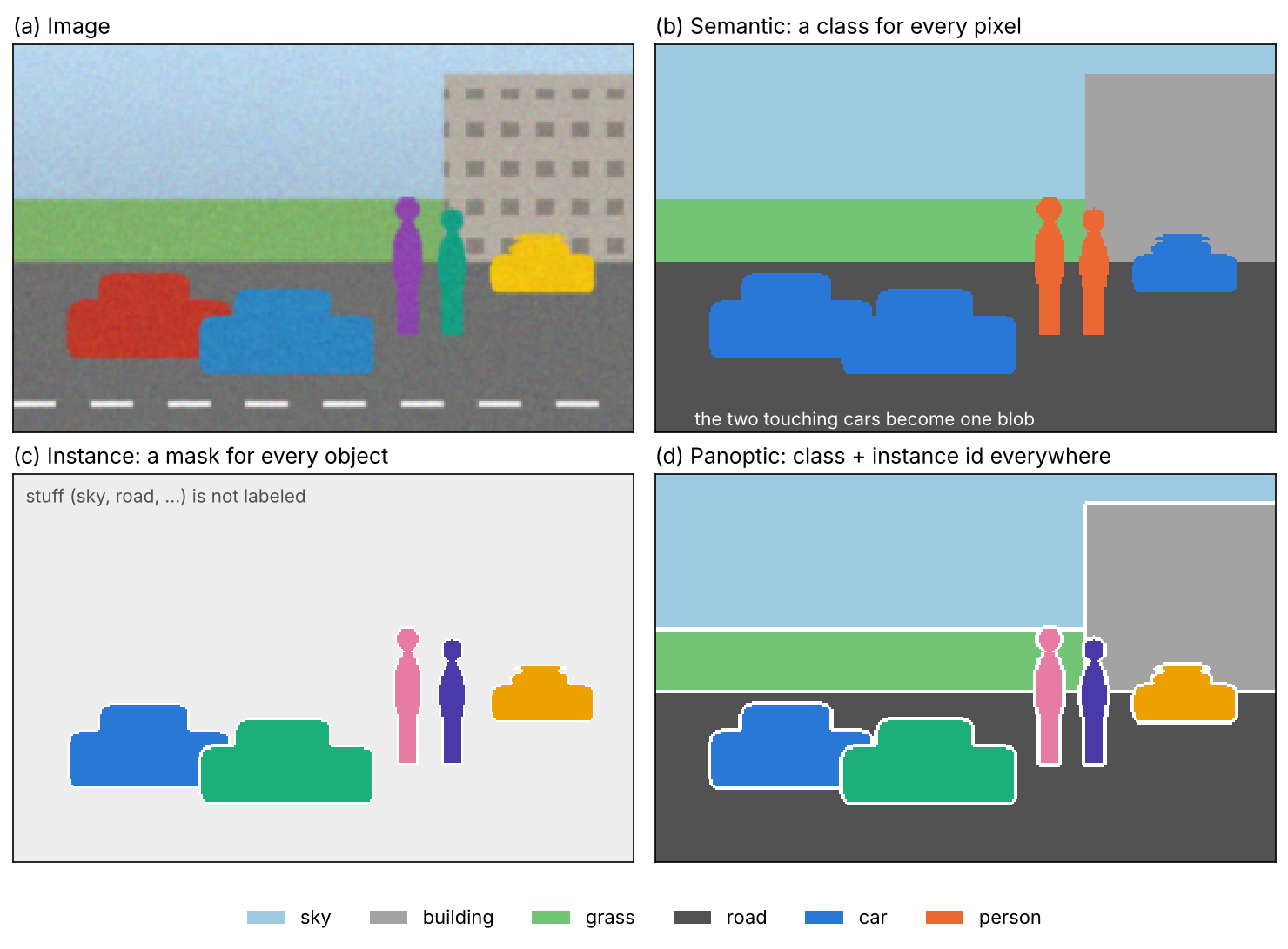
| Semantic | Instance | Panoptic | |
|---|---|---|---|
| Labels | class per pixel | mask + class + score per object | (class, instance id) per pixel |
| Classes covered | stuff and things | things only | stuff and things |
| Overlaps allowed | no | yes | no |
| Confidence scores | no | yes | no |
| Standard metric | mean IoU | mask AP | panoptic quality (PQ) |
The table explains why the three tasks long had separate methods: their outputs have different shapes, and each metric rewards something different. Most of this chapter follows that history: per-pixel classifiers for semantic segmentation first, then detector-based instance segmentation, then the panoptic task that forced the two to meet, and finally one architecture that handles all three.
From a classifier to a per-pixel classifier
Plain version. Keep spatial features instead of globally pooling them. Predict a grid of class scores, then upsample it to the image size.
Fully convolutional networks
Long, Shelhamer and Darrell’s fully convolutional network (FCN) [5] replaced the fully connected layers of a classification network with convolutions. A convolution works on an input of any size, so the network now maps an image to a score map
where is the number of classes and is the output stride, the ratio between the input resolution and the score-map resolution. A classification backbone pools and strides repeatedly; for the networks FCN started from, , so a image yields a grid of class scores. Each score vector summarizes a large window of the image, which is good for recognizing what is there, but one cell covers pixels, which is bad for saying exactly where a boundary runs.
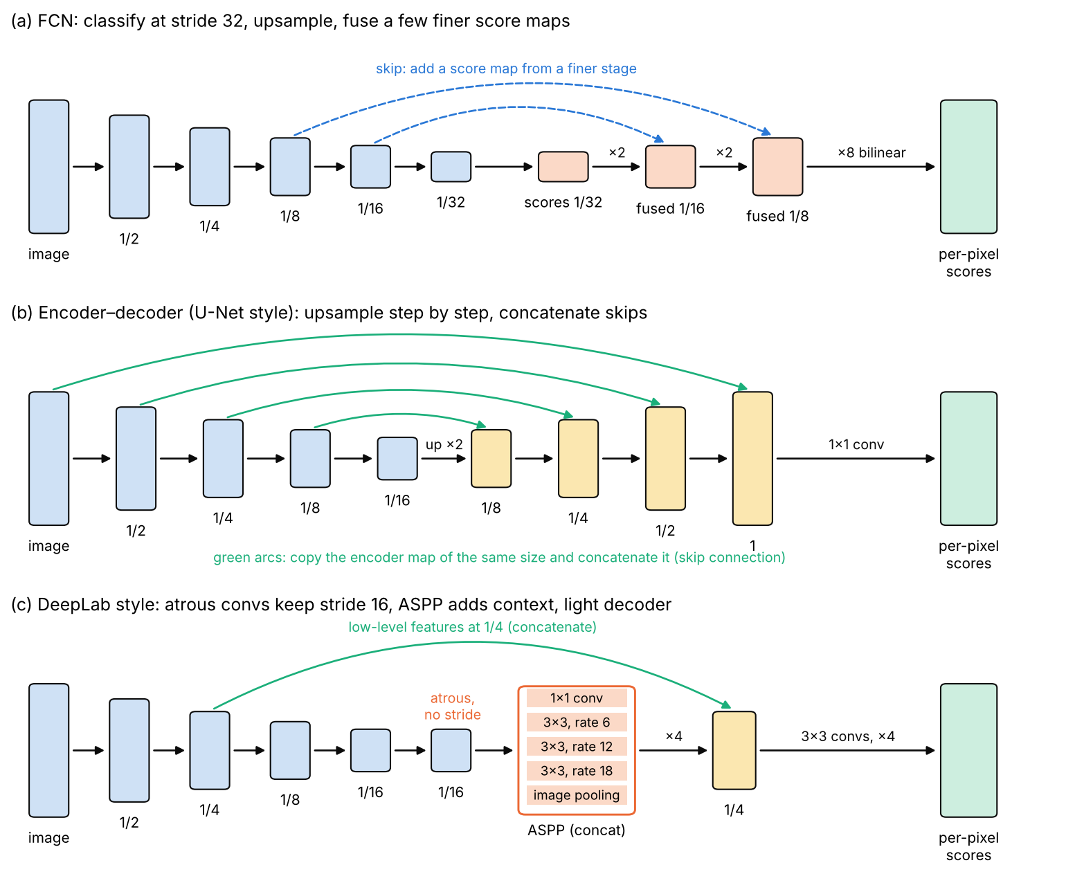
FCN trains the whole network end to end with a per-pixel cross-entropy loss after upsampling to the input size, starting from weights pretrained for classification. To recover detail, it fuses predictions from finer layers: the stride-32 scores are upsampled by 2 and added to a score map computed from the stride-16 layer, and again for stride 8. The paper calls the three versions FCN-32s, FCN-16s and FCN-8s, and shows that each finer fusion gives more detailed outlines [5]. Its summary of the idea is a good one-liner for the whole field: combine “what” from a deep, coarse layer with “where” from a shallow, fine layer. DLCV 01 introduces the same idea in its section on encoder–decoders.
Upsample the scores, not the labels
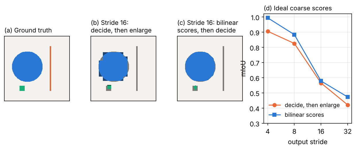
Plain version. If you decide the class at low resolution and then enlarge the decision, every boundary becomes a staircase of blocks. If you first enlarge the scores smoothly and then decide per pixel, the boundaries fall between grid points.
Bilinear interpolation computes the score at a fine position from the four nearest coarse cells. For a fine pixel that sits at fractional coarse coordinates with integers and ,
where is the score map of class and the interpolated score. The predicted label is . FCN implements upsampling as a strided transposed convolution initialized to bilinear interpolation, and lets the network learn it [5]; transposed convolution is explained in ML 03. Most later models simply use fixed bilinear upsampling for the last step.
The experiment below isolates the effect of output stride. It builds an ideal coarse score map, the fraction of each class inside each cell, an idealized output for a stride- head, and compares the two orders of “enlarge” and “decide”.
Code · Python · 28 lines
import numpy as np
from scipy import ndimage as ndi

# Synthetic ground truth: 0 background, 1 large disk, 2 thin bar, 3 small square
H = W = 256
yy, xx = np.mgrid[0:H, 0:W]
gt = np.zeros((H, W), int)
gt[(yy - 120) ** 2 + (xx - 90) ** 2 < 60 ** 2] = 1
gt[40:216, 178:184] = 2                        # 6 pixels wide
gt[196:216, 60:80] = 3                         # 20 x 20 pixels
K = 4

def iou_per_class(gt, pred, K):
    return np.array([((gt == k) & (pred == k)).sum() / ((gt == k) | (pred == k)).sum()
                     for k in range(K)])

onehot = np.stack([(gt == k).astype(float) for k in range(K)])
print("stride | nearest labels: mIoU (per class) | bilinear scores: mIoU (per class)")
for s in [4, 8, 16, 32]:
    # ideal stride-s scores: the class fractions inside each s x s cell
    coarse = onehot.reshape(K, H // s, s, W // s, s).mean(axis=(2, 4))
    # (a) decide at low resolution, then enlarge the label map
    lab_nn = np.kron(coarse.argmax(0), np.ones((s, s), int))
    # (b) enlarge the scores with bilinear interpolation, then decide per pixel
    up = np.stack([ndi.zoom(c, s, order=1, mode="nearest", grid_mode=True) for c in coarse])
    lab_bi = up.argmax(0)
    a, b = iou_per_class(gt, lab_nn, K), iou_per_class(gt, lab_bi, K)
    print(f"{s:6d} | {a.mean():.3f} {np.round(a, 2)} | {b.mean():.3f} {np.round(b, 2)}")
Output
stride | nearest labels: mIoU (per class) | bilinear scores: mIoU (per class)
     4 | 0.906 [0.99 0.97 0.67 1.  ] | 0.994 [1.   1.   0.99 0.99]
     8 | 0.825 [0.98 0.93 0.75 0.64] | 0.883 [0.99 0.99 0.7  0.86]
    16 | 0.565 [0.95 0.89 0.   0.41] | 0.578 [0.97 0.97 0.   0.37]
    32 | 0.421 [0.92 0.76 0.   0.  ] | 0.473 [0.96 0.93 0.   0.  ]
Three lessons come out of this toy run (the numbers are from the code above, not from any paper). Bilinear upsampling of scores is almost free and always at least as good for the large disk. But no upsampling can bring back what the coarse grid never saw: at stride 16 the 6-pixel bar is a minority in every cell and vanishes, and at stride 32 the 20-pixel square vanishes too. Thin and small structures need a small output stride or a decoder that brings fine features back. And mean IoU punishes those losses heavily, because the bar and the square count as much as the background (Figure 2).
Encoder–decoders and skip connections
Plain version. A decoder increases resolution gradually and reuses matching encoder features through skips to recover detail.
U-Net [6] made this symmetric: a contracting encoder of convolutions and downsampling, an expanding decoder of upsampling and convolutions, and at each level a skip connection that concatenates the encoder’s feature map to the decoder’s. The encoder supplies what, the skips supply where. The paper’s design choices (unpadded convolutions, the overlap-tile strategy, a weighted loss for touching cells and strong elastic augmentation) are covered in the U-Net reading guide of IP 10.
Optional: U-Net: a reading guide to the paper (in the Paper guides of IP 10). What the paper claims, the output-size arithmetic of valid convolutions, and how to read its tables.
The opposite design keeps the decoder light. DeepLabv3+ [7] runs the encoder to output stride 16, upsamples its features by 4, concatenates low-level features from the backbone at stride 4 (after a convolution that reduces their channels), refines with a few convolutions and upsamples by 4 again. The paper motivates the decoder by noting that a plain 16-fold bilinear upsampling, a “naive decoder”, may not recover object details. Figure 3 compares the three shapes: FCN’s few fused score maps, U-Net’s full ladder, and DeepLab’s context module plus a single skip.
Context without losing resolution
Plain version. To label a pixel you need two things that pull in opposite directions: a wide view (is this grey patch a road or a wall?) and fine resolution (where exactly does the road end?). Atrous convolution and pooling pyramids give the wide view without shrinking the map.
Atrous (dilated) convolution
Downsampling is the usual way a CNN grows its receptive field, the region of the input that one output can see (DLCV 01 and ML 03 derive it). An atrous convolution (“à trous”, with holes) spreads the taps of a small kernel apart instead. In 1-D, DeepLab [8] defines the output of an atrous convolution of input with a filter of length as
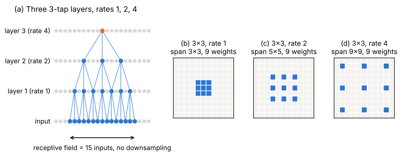
where indexes output positions and is the rate: the input is sampled every positions. Rate is ordinary convolution. A kernel with rate covers pixels per side with the same weights and the same cost [8]. Yu and Koltun [9] called the same operation a dilated convolution and showed that stacking dilations that double from layer to layer grows the receptive field exponentially without losing resolution.
The DeepLab recipe is to set the stride of the last downsampling layer to 1 and replace the convolutions that follow by atrous convolutions with rate 2, so that they still see the same image region with the same pretrained weights; repeating this for one more stage doubles the density again [8]. Typical models output stride 8 or 16 instead of 32 [10]. The price is compute and memory: stride 8 has four times as many positions as stride 16 in the last stages.
Code · Python · 25 lines
import numpy as np

def atrous_1d(x, w, r):
    """y[i] = sum_k x[i + r*k] w[k] (DeepLab's Eq. 1), taps centred, zero padding."""
    K = len(w); c = K // 2
    xp = np.pad(x, r * c)
    return np.array([sum(xp[i + r * (k)] * w[k] for k in range(K)) for i in range(len(x))])

x = np.zeros(21); x[10] = 1.0                   # an impulse in the middle
w = np.array([1.0, 1.0, 1.0])
for r in [1, 2, 4]:
    print(f"rate {r}: taps at offsets {[(k - 1) * r for k in range(3)]},",
          "response", atrous_1d(x, w, r).astype(int))

def receptive_field(kernels, rates, strides):
    """Receptive field (in input pixels) of a stack of conv layers."""
    rf, jump = 1, 1                              # jump = distance between neighbouring outputs, in input pixels
    for k, r, s in zip(kernels, rates, strides):
        rf += (r * (k - 1)) * jump
        jump *= s
    return rf, jump

print("three 3x3, rates 1,1,1:", receptive_field([3, 3, 3], [1, 1, 1], [1, 1, 1]))
print("three 3x3, rates 1,2,4:", receptive_field([3, 3, 3], [1, 2, 4], [1, 1, 1]))
print("three 3x3, stride 2   :", receptive_field([3, 3, 3], [1, 1, 1], [2, 2, 2]))
Output
rate 1: taps at offsets [-1, 0, 1], response [0 0 0 0 0 0 0 0 0 1 1 1 0 0 0 0 0 0 0 0 0]
rate 2: taps at offsets [-2, 0, 2], response [0 0 0 0 0 0 0 0 1 0 1 0 1 0 0 0 0 0 0 0 0]
rate 4: taps at offsets [-4, 0, 4], response [0 0 0 0 0 0 1 0 0 0 1 0 0 0 1 0 0 0 0 0 0]
three 3x3, rates 1,1,1: (7, 1)
three 3x3, rates 1,2,4: (15, 1)
three 3x3, stride 2   : (15, 8)
The last two lines are the whole argument for atrous convolution. Three layers with rates 1, 2, 4 see 15 input pixels, exactly as many as three stride-2 layers, but they keep one output per input pixel (jump 1) instead of one per 8 pixels (Figure 4).
Dilation has a catch. A single dilated layer only reads a sparse lattice of inputs, and stacking layers whose rates share a common factor leaves holes that no path ever reaches, a checkerboard artifact that Wang et al. call gridding [11]. The fix is to choose rates such as 1, 2, 5 that fill each other’s gaps.
Optional: Gridding in stacked dilated convolutions (in the Supplementary notes). Which rate sequences leave holes, the hybrid-dilation rule, and a check in code.
Multi-scale context: ASPP and pyramid pooling
Plain version. Objects come at many sizes, and what a pixel is often depends on what surrounds it. So look at each position through several windows of different sizes at once, including one that sees the whole image, and let the network combine the answers.
Atrous spatial pyramid pooling (ASPP) [8] applies several atrous convolutions with different rates in parallel to the same feature map and fuses their outputs, which probes the image at several effective scales. DeepLabv3 [10] uses one convolution and three convolutions with rates 6, 12 and 18 at output stride 16 (rates doubled at stride 8), plus an image-level feature: global average pooling of the whole map, a convolution, and bilinear upsampling back. The reason for the image-level branch is a boundary effect the paper points out: as the rate approaches the feature-map size, more and more of the taps fall outside the map, and the filter degenerates to a filter that only uses its centre weight. The snippet counts this on a map.
Code · Python · 8 lines
import numpy as np

n = 65                                           # feature map is n x n
for r in [1, 6, 12, 18, 24, 36, 64]:
    pos = np.arange(n)
    inside_1d = np.array([[(0 <= p + r * d < n) for d in (-1, 0, 1)] for p in pos]).sum(1)
    mean_taps = np.mean(np.outer(inside_1d, inside_1d))   # taps inside the map, averaged over positions
    print(f"rate {r:2d}: mean valid taps {mean_taps:.2f} of 9")
Output
rate  1: mean valid taps 8.82 of 9
rate  6: mean valid taps 7.93 of 9
rate 12: mean valid taps 6.92 of 9
rate 18: mean valid taps 5.98 of 9
rate 24: mean valid taps 5.11 of 9
rate 36: mean valid taps 3.58 of 9
rate 64: mean valid taps 1.06 of 9
At rate 64 a “3×3” filter is, on average, a single tap. Global pooling is the cheap and reliable way to get image-wide context.
The Pyramid Scene Parsing Network (PSPNet) [12] reaches the same goal with pooling instead of dilation. Its pyramid pooling module pools the final feature map into , , and grids, reduces each with a convolution, upsamples all of them back and concatenates them with the original features. The paper motivates it with errors of an FCN baseline on scene parsing, such as a “mismatched relationship”: a boat on a river labeled as a car, although a car is seldom over a river [12].
Early DeepLab versions also sharpened boundaries after the network with a fully connected conditional random field, which encourages pixels of similar colour and position to share a label [8]. DeepLabv3 improves on the earlier versions without it [10].
Optional: Dense CRF post-processing (in the Supplementary notes). The energy, its two Gaussian kernels, and why mean-field inference makes it fast.
Attention as context
A transformer gives every token a view of every other token in each layer, so “context” no longer needs a special module (ML 05 explains the Vision Transformer, ViT [13]). The catch is resolution: plain ViT has one coarse token grid, and global attention over many tokens is costly. SegFormer [14] is a widely used answer for semantic segmentation. Its encoder is hierarchical, producing multi-scale features like a CNN, uses a reduced attention that shortens the key and value sequences, and needs no positional encoding, which avoids interpolating position codes when the test resolution differs from the training one. Its decoder is only a few MLP layers that fuse the multi-scale features. Hierarchical vision transformers are covered in ML 05.
Losses for dense prediction
Plain version. A segmenter is trained by comparing its per-pixel probabilities with the true label map. Averaging a classification loss over pixels is the default, but when one class covers 99% of the image, that average mostly measures the easy class.
Per-pixel cross-entropy. With the softmax probability of class at pixel and the true class,
where is the set of labeled (non-void) pixels and an optional weight per class, for example inversely proportional to the class frequency. Void pixels are simply left out of the sum; most frameworks implement this with an “ignore index”.
Dice loss. Milletari et al. [15] proposed to maximize the Dice coefficient between a soft prediction and the binary ground truth directly, as an alternative to re-weighting samples, because the anatomy of interest often occupies only a small part of a medical volume and training then tends to predict background everywhere. For foreground probabilities and labels over pixels, their form is
A common variant uses in the denominator; with binary and both equal the overlap measure , a close relative of IoU. For several classes, the Dice loss is computed per class and averaged. Because is a ratio over the whole image, a small object counts as much as a large background.
Focal loss. The focal loss [16] multiplies the cross-entropy of each pixel by , where is the probability of the true class, so that easy pixels contribute little; it is derived in DLCV 03. Combinations are common: MaskFormer, discussed below, trains each binary mask with a weighted sum of a focal loss and a Dice loss [17].
The experiment compares the losses on a 64×64 image whose foreground is a disk of 49 pixels, for three candidate predictions. “IoU@0.5” thresholds the probabilities at 0.5 and computes the IoU that an evaluation would report.
Code · Python · 40 lines
import numpy as np

H = W = 64
yy, xx = np.mgrid[0:H, 0:W]
r2 = (yy - 32) ** 2 + (xx - 32) ** 2
g = (r2 <= 4 ** 2).astype(float)                # small foreground disk
print(f"foreground pixels: {int(g.sum())} of {g.size} ({100 * g.mean():.1f}%)")

def bce(p, g):
    return -np.mean(g * np.log(p) + (1 - g) * np.log(1 - p))

def weighted_bce(p, g):                          # weight each class by inverse frequency
    wf, wb = 0.5 / g.mean(), 0.5 / (1 - g.mean())
    return -np.mean(wf * g * np.log(p) + wb * (1 - g) * np.log(1 - p))

def focal(p, g, gamma=2.0):
    pt = np.where(g == 1, p, 1 - p)
    return -np.mean((1 - pt) ** gamma * np.log(pt))

def soft_dice_loss(p, g, eps=1e-6):
    return 1 - (2 * (p * g).sum() + eps) / (p.sum() + g.sum() + eps)

def iou_at_half(p, g):                           # the metric we actually report
    m = p > 0.5
    return (m & (g == 1)).sum() / (m | (g == 1)).sum()

preds = {
    "all background (p=0.05)":  np.full((H, W), 0.05),
    "right shape, timid (0.4)": np.where(g == 1, 0.4, 0.05),
    "bloated, confident (0.9)": np.where(r2 <= 8 ** 2, 0.9, 0.05),
}
print(f"{'prediction':26s} {'BCE':>6s} {'wBCE':>6s} {'focal':>6s} {'Dice':>6s} {'IoU@0.5':>8s}")
for name, p in preds.items():
    print(f"{name:26s} {bce(p, g):6.3f} {weighted_bce(p, g):6.3f} "
          f"{focal(p, g):6.3f} {soft_dice_loss(p, g):6.3f} {iou_at_half(p, g):8.3f}")

# Where does the BCE gradient come from? dL/dz = p - g per pixel (z = logit)
p = preds["all background (p=0.05)"]
grad = np.abs(p - g)
print(f"share of |BCE gradient| from background pixels: {grad[g == 0].sum() / grad.sum():.2f}")
Output
foreground pixels: 49 of 4096 (1.2%)
prediction                    BCE   wBCE  focal   Dice  IoU@0.5
all background (p=0.05)     0.087  1.524  0.032  0.981    0.000
right shape, timid (0.4)    0.062  0.484  0.004  0.855    0.000
bloated, confident (0.9)    0.133  0.119  0.068  0.791    0.249
share of |BCE gradient| from background pixels: 0.81
Read the table row by row (all numbers are from this toy run). Plain binary cross-entropy (BCE) prefers “all background” to the bloated prediction, the only one that finds the object at the 0.5 threshold, because the bloated mask is wrong on about 150 background pixels and those outnumber the object. The unweighted focal loss, without the class weight , makes the same choice. Class-weighted BCE and Dice both rank the bloated prediction best and “all background” worst, in the same order as the IoU. The last line shows why plain BCE behaves this way: 81% of its gradient comes from background pixels that are already almost right. Note also how harshly soft Dice treats the timid prediction: the 4,047 background pixels at add about 202 to the denominator, more than four times the object’s area, so a soft prediction must be confident on the background too.
In practice, cross-entropy (often with class weights or the focal modulation) is the default for natural-scene semantic segmentation, Dice or a Dice + cross-entropy sum is common for medical images with small structures, and mask-based models train each mask with Dice + focal. Losses that also penalize boundary or topology errors exist; three built from active-contour energies are summarized in IP 11’s Supplementary notes.
Optional: The gradient of the soft Dice loss (in the Supplementary notes). The derivative in closed form, why every background pixel gets the same push, and edge cases such as empty masks.
Measuring semantic segmentation
Plain version. Count, over the whole test set, how many pixels of each true class were given each predicted class. Every common score is a different summary of that table. The standard one, mean IoU, asks for each class “of all pixels that are this class or were called this class, what fraction got it right?”, and then averages over classes.
Let be the number of pixels of true class predicted as class , accumulated over all test images, and the number of pixels of class . FCN [5] defines four metrics, with classes:
In the IoU of class , the numerator counts true positives and the denominator counts the union of true and predicted pixels: (true positives plus misses) plus (false alarms). Mean IoU (mIoU) is the standard metric of PASCAL VOC, Cityscapes and ADE20K.
Code · Python · 26 lines
import numpy as np

def confusion(gt, pred, K, ignore=255):
    """K x K matrix: rows = true class, columns = predicted class; 'ignore' pixels are skipped."""
    keep = gt != ignore
    return np.bincount(K * gt[keep] + pred[keep], minlength=K * K).reshape(K, K)

def seg_metrics(C):
    tp = np.diag(C).astype(float)
    t = C.sum(1)                    # pixels of each true class
    p = C.sum(0)                    # pixels predicted as each class
    iou = tp / (t + p - tp)
    return {"pixel acc": tp.sum() / C.sum(), "mean acc": np.mean(tp / t),
            "mIoU": iou.mean(), "fwIoU": (t * iou).sum() / t.sum(), "IoU": np.round(iou, 3)}

# Toy: road (0) covers most of the image, car (1) is medium, pole (2) is thin
H, W = 120, 160
gt = np.zeros((H, W), int)
gt[60:100, 40:90] = 1
gt[10:110, 130:133] = 2
pred = gt.copy()
pred[60:100, 86:90] = 0                         # car slightly too short
pred[10:110, 130:133] = 0                       # the pole is missed entirely
m = seg_metrics(confusion(gt, pred, 3))
for k, v in m.items():
    print(f"{k:9s}: {v:.3f}" if np.isscalar(v) else f"{k:9s}: {v}")
Output
pixel acc: 0.976
mean acc : 0.640
mIoU     : 0.631
fwIoU    : 0.953
IoU      : [0.974 0.92  0.   ]
Missing the pole entirely costs 1.6% of pixel accuracy and almost nothing in frequency-weighted IoU, but a third of the mean IoU. That is why mIoU, which weighs every class equally, is the headline number. Four practical details matter when you compare papers:
- The confusion matrix is accumulated over the whole dataset, then the IoUs are computed. Averaging per-image IoUs gives a different number.
- Void pixels are excluded through the ignore label, as in
confusionabove. - mIoU still favours large objects within a class: one large car outweighs ten small ones. Cityscapes therefore also reports an instance-level iIoU, in which each pixel’s contribution is weighted by the ratio of the class’s average instance size to the size of its ground-truth instance [18].
- Region overlap is insensitive to boundary quality on large objects, where a few pixels of boundary error hardly change the IoU. Boundary IoU [19] measures overlap only in a thin band along the contours.
Optional: Boundary IoU in detail (in the Supplementary notes). Its definition, the band width, and a check in code that it scores the same boundary error equally on small and large objects.
Instance segmentation
Plain version. Instance segmentation is detection with an outline. The dominant approach finds each object first, as a detector would, and then segments the inside of its box.
Detect, then segment: Mask R-CNN
Mask R-CNN [20] adds a small fully convolutional mask branch to the two-stage detector Faster R-CNN [21], which DLCV 03 explains together with RoIAlign. For each region of interest, the branch predicts binary masks of size , one per class ( in the paper’s variant built on a feature pyramid network, FPN [22]), and the loss uses a per-pixel sigmoid and the average binary cross-entropy on the mask of the ground-truth class only. Mask and class prediction are therefore decoupled: the box branch chooses the class, and masks of different classes do not compete, unlike the per-pixel softmax of an FCN; the paper’s ablation finds that the per-class sigmoid gives large gains over a softmax [20]. At test time the mask of the predicted class is resized to the box and binarized at 0.5.
Optional: RoI pooling versus RoIAlign (in the Supplementary notes of DLCV 03). Why rounding the box to the feature grid shifts masks, and the bilinear sampling that fixes it.
The fixed grid is also Mask R-CNN’s weakness: a large object’s outline is drawn from a few hundred cells and comes out oversmoothed. PointRend [23] treats mask prediction like rendering in computer graphics: it starts from a coarse mask, repeatedly upsamples it bilinearly, and recomputes predictions only at the most uncertain points of the denser grid (for a binary mask, those with probabilities closest to 0.5), which lie mostly along the boundary.
Other routes exist. Bottom-up methods first predict per-pixel quantities, such as an embedding vector or a distance to the object centre, and then group pixels into instances; a watershed on a predicted distance map, with markers found by the network, is the learned version of the marker-controlled watershed of IP 10. And query-based methods predict a set of masks directly, as described in the mask-classification section below.
Mask AP
Instance segmentation is scored exactly like detection, with the COCO average precision of DLCV 03, except that the IoU between a prediction and a ground-truth object is computed on masks instead of boxes [20]. The metric needs a confidence score per mask, because AP ranks predictions, and it allows overlapping masks: a detector may output several overlapping hypotheses and is only penalized for those that do not match. This is why instance outputs cannot be used as a panoptic map without further processing.
Panoptic segmentation
Plain version. The panoptic task asks for one coherent picture: every pixel labeled, stuff and things alike, no overlaps, and a metric that treats a sky region and a car the same way.
The task and its metric
Kirillov et al. [4] defined the task (the format is the one given in “Three tasks, one label map”) together with a metric, panoptic quality (PQ). PQ is computed in two steps.
1. Matching. A predicted segment and a ground-truth segment of the same class match only if their IoU is strictly greater than 0.5. Because segments of a panoptic map cannot overlap, this match is unique: if and are disjoint predictions, then , since each and the two intersections share no pixel. So at most one prediction can exceed 0.5 for each , and vice versa [4]. No optimal assignment step is needed.
2. Scoring. For each class, the matches split the segments into true positives (matched pairs), false positives (unmatched predictions) and false negatives (unmatched ground-truth segments). Then
where the sums run over matched pairs and counts elements of a set. SQ is the average IoU of matched segments, and RQ is the familiar F1 score of detection. PQ is computed per class and averaged over classes, so a rare class counts as much as a frequent one; every segment counts equally regardless of its area. and average over stuff and thing classes only. Void pixels are removed from predictions before matching, and unmatched predictions that consist mostly of void (or of a “crowd” region of the same class) are not counted as false positives [4]. The two factors are not independent, since SQ is measured only on the matched segments, so always report all three.
The code implements this matching and scoring on the toy scene of Figure 5 (void handling reduced to its simplest form).
Code · Python · 45 lines
import numpy as np

def panoptic_quality(gt_seg, gt_cls, pr_seg, pr_cls):
    """gt_seg/pr_seg: integer segment-id maps (0 = void); *_cls: dict segment id -> class.
    Matches segments of the same class with IoU > 0.5 and returns per-class (PQ, SQ, RQ, TP, FP, FN)."""
    out = {}
    for c in sorted(set(gt_cls.values()) | set(pr_cls.values())):
        g_ids = [i for i, k in gt_cls.items() if k == c]
        p_ids = [i for i, k in pr_cls.items() if k == c]
        ious, matched_p = [], set()
        for gi in g_ids:
            G = gt_seg == gi
            for pj in p_ids:
                P = (pr_seg == pj) & (gt_seg != 0)          # ignore predicted pixels on void
                iou = (G & P).sum() / (G | P).sum()
                if iou > 0.5:                                # unique by the matching theorem
                    ious.append(iou); matched_p.add(pj)
        tp = len(ious); fn = len(g_ids) - tp; fp = len(p_ids) - len(matched_p)
        sq = np.mean(ious) if tp else 0.0
        rq = tp / (tp + 0.5 * fp + 0.5 * fn)
        out[c] = (sq * rq, sq, rq, tp, fp, fn)
    return out

H, W = 100, 200
SKY, ROAD, CAR, PERSON = 0, 1, 2, 3
def scene(boxes, sky_rows):
    seg = np.full((H, W), 2); seg[:sky_rows] = 1          # segment 1 = sky, 2 = road
    cls = {1: SKY, 2: ROAD}
    for sid, (c, r0, r1, c0, c1) in enumerate(boxes, start=3):
        seg[r0:r1, c0:c1] = sid; cls[sid] = c
    return seg, cls

gt_seg, gt_cls = scene([(CAR, 50, 80, 10, 55), (CAR, 50, 80, 65, 110),
                        (CAR, 38, 52, 125, 150), (PERSON, 30, 80, 165, 185)], sky_rows=30)
pr_seg, pr_cls = scene([(CAR, 52, 80, 13, 55),             # car A, slightly off
                        (CAR, 55, 80, 65, 96),             # car B, too small
                        (CAR, 84, 97, 110, 150),           # a car that is not there
                        (PERSON, 30, 52, 165, 185),        # the person, split in two
                        (PERSON, 52, 80, 165, 185)], sky_rows=33)   # car C is missed
names = ["sky", "road", "car", "person"]
res = panoptic_quality(gt_seg, gt_cls, pr_seg, pr_cls)
for c, (pq, sq, rq, tp, fp, fn) in res.items():
    print(f"{names[c]:6s} PQ {pq:.3f} = SQ {sq:.3f} x RQ {rq:.3f}  (TP {tp}, FP {fp}, FN {fn})")
pqs = np.array([v[0] for v in res.values()])
print(f"PQ {pqs.mean():.3f} | PQ_stuff {pqs[:2].mean():.3f} | PQ_things {pqs[2:].mean():.3f}")
Output
sky    PQ 0.917 = SQ 0.917 x RQ 1.000  (TP 1, FP 0, FN 0)
road   PQ 0.805 = SQ 0.805 x RQ 1.000  (TP 1, FP 0, FN 0)
car    PQ 0.482 = SQ 0.723 x RQ 0.667  (TP 2, FP 1, FN 1)
person PQ 0.373 = SQ 0.560 x RQ 0.667  (TP 1, FP 1, FN 0)
PQ 0.644 | PQ_stuff 0.861 | PQ_things 0.428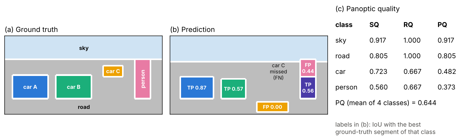
The toy shows how PQ reads errors (numbers from this run). The split person still gets a match, because the lower piece covers 56% of it, but the upper piece becomes a false positive: splitting an object costs recognition quality, not just segmentation quality. Car B, at IoU 0.57, counts as fully recognized, but its low IoU pulls the car’s SQ down. A missed car and an invented car each cost half a segment in the denominator.
Early panoptic systems: merge two outputs
Plain version. The first panoptic systems simply ran a semantic segmenter and an instance segmenter and pasted the results together.
The panoptic paper’s own baseline [4] does this with a non-maximum-suppression-like procedure. It sorts the instance masks by confidence, drops low-scoring ones, and walks down the list: each mask loses the pixels already claimed by earlier masks and is kept only if enough of it remains. The surviving thing segments are then combined with the semantic map, and any pixel claimed by both a thing and a stuff class goes to the thing. Panoptic FPN [24] then put both tasks into one network: a Mask R-CNN with a feature pyramid network (FPN [22], see DLCV 03) plus a light semantic branch that upsamples and sums all pyramid levels at 1/4 scale. The semantic branch predicts the stuff classes plus a single “other” class for all thing pixels, so the two branches do not fight over objects.
Optional: Panoptic Segmentation: a reading guide (in the Paper guides). How the paper defines the task and metric, what its human-consistency study shows, and how to read its tables.
Mask classification: one model for all three tasks
Plain version. Instead of asking “what class is this pixel?”, ask “which regions are there, and what is each region?”. Predict a fixed number of candidate masks and one class (or “nothing”) for each. A semantic map, a set of instances and a panoptic map are then just different ways of reading the same list.
MaskFormer
Cheng, Schwing and Kirillov [17] call the FCN formulation per-pixel classification and the Mask R-CNN and DETR formulation mask classification. Their observation is that mask classification is general enough for semantic segmentation too. MaskFormer predicts a set of probability–mask pairs , where is a distribution over classes plus a “no object” label , and is a soft mask. Three modules produce them:
- A backbone and a pixel decoder produce per-pixel embeddings , where is the embedding dimension.
- A transformer decoder turns learnable queries into per-segment embeddings by attending to the image features, as in DETR [25].
- A linear classifier gives , and a small MLP gives a mask embedding . The mask is a dot product followed by a sigmoid,
where is the logistic sigmoid and a pixel position.
Training matches predictions to ground-truth segments one to one, as DETR does for boxes (DLCV 03), but with a matching cost built from class probabilities and mask losses instead of boxes. Matched predictions get a cross-entropy class loss and a focal + Dice mask loss; unmatched ones are trained to predict [17].
At inference, two rules read the same output in different ways [17]. Semantic inference marginalizes over queries, , with ranging over the real classes. Panoptic inference assigns each pixel to one query, , where is the most likely class of query , so two queries of the same class give two instances. The snippet runs both rules on a tiny example.
Code · Python · 33 lines
import numpy as np

rng = np.random.default_rng(0)
# Ground-truth layout of a tiny 6 x 10 image: sky on top, road below, two cars on the road
region = np.zeros((6, 10), int)               # 0 sky, 1 road, 2 car A, 3 car B
region[2:] = 1
region[3:5, 1:4] = 2
region[3:5, 6:9] = 3

# Pixel decoder output: a C_E = 4 dimensional embedding per pixel (here: noisy one-hot of the region)
E_pixel = 6 * np.eye(4)[region].transpose(2, 0, 1) - 3 + 0.5 * rng.standard_normal((4, 6, 10))

# Transformer decoder output for N = 5 queries: a mask embedding and class probabilities
# over K = 3 classes (sky, road, car) plus "no object" (last column)
E_mask = np.array([[1, 0, 0, 0], [0, 1, 0, 0], [0, 0, 1, 0], [0, 0, 0, 1], [.2, .2, .2, .2]], float)
p = np.array([[.90, .05, .03, .02],          # query 0: sky
              [.05, .85, .05, .05],          # query 1: road
              [.02, .08, .85, .05],          # query 2: a car
              [.03, .07, .75, .15],          # query 3: another car
              [.05, .05, .05, .85]])         # query 4: nothing

m = 1 / (1 + np.exp(-np.einsum("nc,chw->nhw", E_mask, E_pixel)))   # N masks, sigmoid(dot product)

# Semantic inference: sum over queries of p_i(c) * m_i, then argmax over the K real classes
sem = np.einsum("nk,nhw->khw", p[:, :3], m).argmax(0)
# Panoptic inference: each pixel goes to the query maximizing p_i(c_i) * m_i (no-object queries dropped)
c_i = p.argmax(1)
keep = c_i != 3
score = p[np.arange(5), c_i][:, None, None] * m
seg = np.where(keep[:, None, None], score, -1).argmax(0)
print("semantic (0 sky, 1 road, 2 car):\n", sem)
print("panoptic segment = query index:\n", seg)
print("query classes:", c_i, "-> car segments:", [int(i) for i in np.unique(seg) if c_i[i] == 2])
Output
semantic (0 sky, 1 road, 2 car):
 [[0 0 0 0 0 0 0 0 0 0]
 [0 0 0 0 0 0 0 0 0 0]
 [1 1 1 1 1 1 1 1 1 1]
 [1 2 2 2 1 1 2 2 2 1]
 [1 2 2 2 1 1 2 2 2 1]
 [1 1 1 1 1 1 1 1 1 1]]
panoptic segment = query index:
 [[0 0 0 0 0 0 0 0 0 0]
 [0 0 0 0 0 0 0 0 0 0]
 [1 1 1 1 1 1 1 1 1 1]
 [1 2 2 2 1 1 3 3 3 1]
 [1 2 2 2 1 1 3 3 3 1]
 [1 1 1 1 1 1 1 1 1 1]]
query classes: [0 1 2 2 3] -> car segments: [2, 3]
The semantic map merges both cars into class 2; the panoptic map keeps them apart as segments 2 and 3, from exactly the same network output. The paper reports that MaskFormer is on par with per-pixel classification on Cityscapes (19 classes) and better on datasets with larger vocabularies [17].
Mask2Former and its successors
Mask2Former [26] kept MaskFormer’s meta-architecture (backbone, pixel decoder, transformer decoder) and changed the decoder so that it trains faster and segments instances well. Its key component is masked attention: each query attends only to the pixels inside the mask it predicted at the previous layer. In layer , with query features ,
where is a linear projection of , and are projections of the image features, and is the previous layer’s mask prediction, resized and binarized at 0.5. Adding before the softmax gives zero attention weight outside the mask. The authors hypothesize that local features suffice to update a query, and that the slow convergence of earlier models came from cross-attention having to learn to focus on the object. Two further changes are a round-robin use of the pixel decoder’s 1/32, 1/16 and 1/8 feature maps in successive decoder layers, for small objects, and computing the mask loss on sampled points instead of full masks, which the paper reports reduces training memory three-fold [26].
Optional: Mask2Former: a reading guide (in the Paper guides). What “universal” means in the paper, its ablations, how to read its comparison tables and the limitations it states.
Two later directions build on this design. OneFormer [27] trains a single model for all three tasks: it derives semantic and instance labels from panoptic annotations, samples one task per training image, and conditions the queries on a “task token”, so that one set of weights serves every task. EoMT [28] removes the task-specific parts altogether. The authors argue that a large plain ViT with extensive pretraining can learn what the adapter, pixel decoder and transformer decoder supplied; they concatenate learnable queries to the patch tokens before the last ViT blocks, which then process both jointly, and report accuracy similar to the more complex models at much higher speed (up to four times faster with ViT-L).
Promptable and open-vocabulary segmentation
Plain version. The models above segment a fixed list of classes they were trained on. Two newer families relax that list. Promptable models segment whatever you point at; open-vocabulary models segment whatever you name.
Promptable segmentation. The Segment Anything Model (SAM) [29] returns a mask for a point, box or rough-mask prompt, and for an ambiguous point (shirt or person?) it returns several valid masks with confidence scores; it was trained on SA-1B, a dataset of over 1 billion masks on 11 million images built with a model-in-the-loop data engine. SAM 2 [30] extends this to video with a streaming memory, and SAM 3 [31] adds promptable concept segmentation: given a short noun phrase or image exemplars, it returns masks and identities for all matching instances. These models are described in DLCV 01 and ML 10, and SAM 2 as a tracker in DLCV 07. In terms of this chapter’s three tasks: SAM’s masks carry no class, so on their own they are neither semantic nor panoptic output; a box from a detector plus SAM gives instance masks; and SAM 3’s concept prompts make it an open-vocabulary instance segmenter. When you read “zero-shot” results with such models, check where the prompts came from: prompts derived from ground-truth boxes give the model a lot of information.
Open-vocabulary segmentation. The key ingredient is a vision–language model such as CLIP [32], whose text encoder maps any class name to an embedding in the same space as image features (ML 10 covers it). Replace a segmenter’s fixed classifier weights with text embeddings of the class names and the vocabulary becomes a list you type at test time. LSeg [33] does exactly this: a transformer image encoder produces per-pixel embeddings, a text encoder embeds the label names, and training aligns each pixel’s embedding with the text embedding of its class, so that unseen labels can be used at test time without retraining. CAT-Seg [34] instead builds a cost volume of cosine similarities between CLIP image and text embeddings and aggregates it, which the authors find lets them fine-tune CLIP’s encoders without overfitting to the training classes, a problem that made most earlier methods freeze CLIP. Zhu and Chen’s survey [35] warns that evaluating “unseen” classes is difficult because the image–text pretraining data may already contain them.
Datasets and benchmarks
Plain version. Pixel labels are expensive, so a few public datasets carry the field. Each one fixes a class list, a stuff/thing split and an evaluation protocol.
| Dataset | Content | Scale and classes (from the papers) | Tasks |
|---|---|---|---|
| PASCAL VOC 2012 [36] | everyday objects | 20 object classes + background (as described in [8]) | semantic |
| Cityscapes [18] | street scenes from 50 cities | 5,000 finely and 20,000 coarsely annotated images; 30 classes, 19 used for evaluation; 8 with instance labels [4] | semantic, instance, panoptic |
| ADE20K [37] | diverse scenes, objects and parts | 20,210 / 2,000 / 3,000 train / val / test images; benchmark of the top 150 classes (SceneParse150); 100 things + 50 stuff for panoptic [4] | semantic, panoptic |
| COCO [38] + COCO-Stuff [39] | everyday scenes | instance masks for 80 thing classes [24]; COCO-Stuff adds pixel labels for 91 stuff classes to all 164K images of COCO 2017; 80 things + 53 stuff in COCO panoptic [17] | instance, semantic, panoptic |
| Mapillary Vistas [40] | street-level images worldwide | 25k images; 28 stuff + 37 thing classes [4] | semantic, instance, panoptic |
Three facts about these datasets shape every result. First, annotation is costly and noisy: the panoptic paper’s human-consistency study, in which two annotations of the same images are scored against each other, gives PQ values well below 100 on all three datasets it examines [4]. Second, class lists are small compared with the vocabulary of the world, which motivates the open-vocabulary models above. Third, domains differ: Cityscapes was recorded in 50 cities, primarily in Germany, and deliberately not in adverse weather [18], so a model trained on it meets different road markings, weather and cameras elsewhere. Bird’s-eye-view map segmentation for driving, which predicts labels on a ground-plane grid instead of the image, is covered in DLCV 03B.
Failure modes and practical advice
Plain version. Segmenters fail in predictable places: where structures are thin or small, along boundaries, on rare classes, and on images unlike the training set.
- Thin and small structures (poles, wires, distant pedestrians) disappear at large output strides, as the first experiment showed. Use output stride 8 or a decoder with high-resolution skips, and evaluate with per-class IoU, not only mIoU.
- Boundaries come out smooth or blocky. Bilinear score upsampling, decoders, point-based refinement such as PointRend [23] and boundary-aware metrics [19] address this.
- Class imbalance biases the network toward frequent classes. Weighted cross-entropy, focal or Dice terms, and sampling images that contain rare classes help (see the loss experiment).
- Context errors: a region labeled with a class that makes no sense in its surroundings (the boat labeled as a car in [12]). Global context modules and attention reduce them.
- Fragmented masks and holes: per-pixel classifiers have no notion of shape. Morphological clean-up of predicted masks (opening, closing, hole filling; see IP 09) is a cheap and common post-processing step.
- High-resolution inputs exceed GPU memory. Run on overlapping tiles and blend the scores, the same overlap-tile idea as U-Net’s.
- Domain shift: performance drops on new cities, weather, sensors or medical scanners. Measure it with a held-out domain, not only a held-out split.
Modern view
What the surveys say
Minaee et al. [1] review the CNN era of semantic and instance segmentation in ten families: fully convolutional networks, convolutional models with graphical models (such as CRFs), encoder–decoders, multi-scale and pyramid networks, R-CNN-based models for instances, dilated convolutions and the DeepLab family, recurrent networks, attention models, generative and adversarial models, and convolutional models combined with active contours. They also review datasets and reported results. Most families appear in this chapter’s sections, with FCN, U-Net, PSPNet, DeepLab and Mask R-CNN as examples.
Li et al. [2] organize transformer-based segmentation around one meta-architecture with a feature extractor, object queries and a transformer decoder, and classify methods by which component they modify: better backbones, cross-attention designs in the decoder, ways of optimizing the queries, and so on. They also cover video and point-cloud segmentation, foundation-model tuning, efficiency and medical segmentation, and they re-evaluate many methods on common benchmarks.
Zhou et al. [3] review more than 300 methods of the foundation-model era, splitting the field into generic segmentation (semantic, instance, panoptic) and promptable segmentation (interactive, referring and few-shot). A central theme is that segmentation knowledge emerges in models trained without masks, such as CLIP, text-to-image diffusion models and self-supervised ViTs, which training-free methods exploit. Zhu and Chen [35] focus on open-vocabulary detection and segmentation and on how hard fair evaluation of “novel” classes is.
The state of the art, 2023–2026
- Universal query-based architectures are the default for closed-vocabulary benchmarks: Mask2Former [26] and its descendants such as OneFormer [27] handle semantic, instance and panoptic segmentation with one design, and specialized per-pixel models remain common where speed or simplicity matters (SegFormer [14], DeepLab-style models [7]).
- Simpler models on larger pretraining: EoMT [28] argues that compute is better spent on scaling a plain ViT encoder than on adding decoders and adapters.
- Promptable foundation models (SAM [29], SAM 2 [30], SAM 3 [31]) turned class-agnostic masks, video propagation and concept prompts into reusable components, and their data engines changed how segmentation datasets are built.
- Open-vocabulary segmentation builds on vision–language models (LSeg [33], CAT-Seg [34]); in many applications a model is now prompted with class names instead of retrained.
Open problems
- Boundaries, small objects and thin structures. Mask2Former’s authors state that it still struggles with small objects [26], and region metrics hide boundary errors on large objects [19].
- One model, trained once. Universal architectures are still often trained separately per task and dataset; Mask2Former trained only on panoptic labels is slightly worse on the instance and semantic metrics than when trained on each task [26].
- Open-vocabulary evaluation depends on prompts and on what the pretraining data contained [35].
- Data. Pixel labels are expensive; the surveys point to scalable data engines, synthetic image–mask pairs from generative models and weak or no supervision as directions, each with its own domain gap [3], [2].
- Efficiency. Foundation-model segmenters are heavy; distillation, compression and parameter-efficient tuning are open engineering problems [3].
- Understanding emergence. Why models trained without masks learn to segment is not well explained [3].
Key takeaways
- Define whether the output needs classes, object identities or both.
- Output stride limits spatial detail; upsample scores before assigning labels.
- Skip-connected decoders restore detail, while dilation, pooling and attention provide context.
- Cross-entropy, focal and Dice losses weight errors differently; choose them for the task’s imbalance and metric.
- mIoU, mask AP and panoptic quality evaluate different output structures and are not interchangeable.
- Mask classification can support several tasks; prompt and vocabulary interfaces change what must be evaluated.
Exercises
- Output stride by hand. A road scene is pixels and a pole is 6 pixels wide. With ideal coarse scores (class fractions per cell) and argmax decisions, at which output strides can the pole survive at all, and why does its position relative to the grid matter? Check your answer by moving the bar in the first snippet by one or two pixels.
Hint
The pole wins a cell only if it covers more than half of the cell’s width, so ; with it survives only in cells where at least 5 of its 6 columns fall inside one 8-pixel cell. At it always covers at least one full cell. Shifting the bar changes which cells it dominates, which is why the bar’s stride-4 IoU in the nearest-label column of the snippet is 0.67, not 1 (a tie at exactly half a cell goes to the background, the first class).
- Atrous arithmetic. (a) What is the effective size of a kernel at rate 12? (b) A backbone stage often starts with stride 2 followed by convolutions. If you remove the stride and use rate 2 instead, what happens to the output stride, the receptive field of the following layers, and the cost of those layers?
Hint
(a) . (b) The output stride halves (for example 32 to 16), every later layer covers the same image region as before (the rate compensates for the denser grid), and the later layers now run on four times as many positions, so their cost grows about four-fold.
- Losses with an empty mask. Modify the loss snippet so that the image contains no foreground. What does each loss return for the “all background (p=0.05)” prediction, and what happens to the soft Dice loss without the
epsterm? How do implementations usually avoid the problem?
Hint
With everywhere, the Dice numerator is 0 (plus eps) and the denominator is , so the loss is almost 1 however good the prediction is; for everywhere it is without eps, and with eps it becomes . iou_at_half also divides 0 by 0 when neither mask has a pixel. Common fixes: add a smoothing constant to numerator and denominator, compute Dice over the whole batch instead of per image, or combine Dice with cross-entropy.
- PQ by hand. In the PQ snippet, replace the two person pieces by a single prediction rows 32 to 80. Predict the new person SQ, RQ and PQ before running the code. Then make car B larger so that its IoU drops below 0.5 by over-segmenting; how do the car’s TP, FP and FN counts change?
Hint
The single person prediction has IoU , so , and . If car B’s IoU falls to 0.5 or below, that pair is no longer a match: car TP drops from 2 to 1, and FP and FN each rise by one.
- Semantic from panoptic, and back. Using the mask-classification snippet, (a) derive the semantic map from the panoptic segment map and check it equals
sem; (b) make query 3 predict “road” instead of “car” with probability 0.6 and explain both outputs. (c) Why can a semantic map not be turned back into a panoptic map in general?
Hint
(a) Map each segment id to its class, c_i[seg]. (b) Query 3’s mask still covers car B, so in the panoptic map car B stays segment 3, but that segment is now labeled road; because a stuff class has a single segment per image, the final output merges it with the road. In the semantic map car B becomes road too. Only one car is left in both. (c) A semantic map has no instance ids: touching objects of one class form one region, and splitting it needs information the map does not contain.
References
- S. Minaee, Y. Boykov, F. Porikli, A. Plaza, N. Kehtarnavaz and D. Terzopoulos, “Image segmentation using deep learning: A survey,” IEEE Transactions on Pattern Analysis and Machine Intelligence, vol. 44, no. 7, 2022. doi · arXiv
- X. Li, H. Ding, H. Yuan, W. Zhang, J. Pang, G. Cheng, K. Chen, Z. Liu and C. C. Loy, “Transformer-based visual segmentation: A survey,” IEEE Transactions on Pattern Analysis and Machine Intelligence, vol. 46, no. 12, 2024. doi · arXiv
- T. Zhou, W. Xia, F. Zhang, B. Chang, W. Wang, Y. Yuan, E. Konukoglu and D. Cremers, “Image segmentation in foundation model era: A survey,” arXiv:2408.12957, 2024. arXiv
- A. Kirillov, K. He, R. Girshick, C. Rother and P. Dollár, “Panoptic segmentation,” in Proc. IEEE/CVF Conference on Computer Vision and Pattern Recognition (CVPR), 2019. doi · arXiv
- J. Long, E. Shelhamer and T. Darrell, “Fully convolutional networks for semantic segmentation,” in Proc. IEEE Conference on Computer Vision and Pattern Recognition (CVPR), 2015. doi · arXiv
- O. Ronneberger, P. Fischer and T. Brox, “U-Net: Convolutional networks for biomedical image segmentation,” in Medical Image Computing and Computer-Assisted Intervention (MICCAI), LNCS vol. 9351, 2015. doi
- L.-C. Chen, Y. Zhu, G. Papandreou, F. Schroff and H. Adam, “Encoder-decoder with atrous separable convolution for semantic image segmentation,” in Proc. European Conference on Computer Vision (ECCV), 2018. doi · arXiv
- L.-C. Chen, G. Papandreou, I. Kokkinos, K. Murphy and A. L. Yuille, “DeepLab: Semantic image segmentation with deep convolutional nets, atrous convolution, and fully connected CRFs,” IEEE Transactions on Pattern Analysis and Machine Intelligence, vol. 40, no. 4, 2018. doi · arXiv
- F. Yu and V. Koltun, “Multi-scale context aggregation by dilated convolutions,” in Proc. International Conference on Learning Representations (ICLR), 2016. arXiv
- L.-C. Chen, G. Papandreou, F. Schroff and H. Adam, “Rethinking atrous convolution for semantic image segmentation,” arXiv:1706.05587, 2017. arXiv
- P. Wang, P. Chen, Y. Yuan, D. Liu, Z. Huang, X. Hou and G. Cottrell, “Understanding convolution for semantic segmentation,” in Proc. IEEE Winter Conference on Applications of Computer Vision (WACV), 2018. doi · arXiv
- H. Zhao, J. Shi, X. Qi, X. Wang and J. Jia, “Pyramid scene parsing network,” in Proc. IEEE Conference on Computer Vision and Pattern Recognition (CVPR), 2017. doi · arXiv
- A. Dosovitskiy, L. Beyer, A. Kolesnikov, D. Weissenborn, X. Zhai, T. Unterthiner et al., “An image is worth 16x16 words: Transformers for image recognition at scale,” in Proc. International Conference on Learning Representations (ICLR), 2021. arXiv
- E. Xie, W. Wang, Z. Yu, A. Anandkumar, J. M. Alvarez and P. Luo, “SegFormer: Simple and efficient design for semantic segmentation with transformers,” in Advances in Neural Information Processing Systems (NeurIPS), 2021. NeurIPS · arXiv
- F. Milletari, N. Navab and S.-A. Ahmadi, “V-Net: Fully convolutional neural networks for volumetric medical image segmentation,” in Proc. Fourth International Conference on 3D Vision (3DV), 2016. doi · arXiv
- T.-Y. Lin, P. Goyal, R. Girshick, K. He and P. Dollár, “Focal loss for dense object detection,” in Proc. IEEE International Conference on Computer Vision (ICCV), 2017. doi
- B. Cheng, A. G. Schwing and A. Kirillov, “Per-pixel classification is not all you need for semantic segmentation,” in Advances in Neural Information Processing Systems (NeurIPS), 2021. NeurIPS · arXiv
- M. Cordts, M. Omran, S. Ramos, T. Rehfeld, M. Enzweiler, R. Benenson, U. Franke, S. Roth and B. Schiele, “The Cityscapes dataset for semantic urban scene understanding,” in Proc. IEEE Conference on Computer Vision and Pattern Recognition (CVPR), 2016. doi · arXiv
- B. Cheng, R. Girshick, P. Dollár, A. C. Berg and A. Kirillov, “Boundary IoU: Improving object-centric image segmentation evaluation,” in Proc. IEEE/CVF Conference on Computer Vision and Pattern Recognition (CVPR), 2021. doi · arXiv
- K. He, G. Gkioxari, P. Dollár and R. Girshick, “Mask R-CNN,” in Proc. IEEE International Conference on Computer Vision (ICCV), 2017. doi · arXiv
- S. Ren, K. He, R. Girshick and J. Sun, “Faster R-CNN: Towards real-time object detection with region proposal networks,” IEEE Transactions on Pattern Analysis and Machine Intelligence, vol. 39, no. 6, 2017. doi
- T.-Y. Lin, P. Dollár, R. Girshick, K. He, B. Hariharan and S. Belongie, “Feature pyramid networks for object detection,” in Proc. IEEE Conference on Computer Vision and Pattern Recognition (CVPR), 2017. doi
- A. Kirillov, Y. Wu, K. He and R. Girshick, “PointRend: Image segmentation as rendering,” in Proc. IEEE/CVF Conference on Computer Vision and Pattern Recognition (CVPR), 2020. doi · arXiv
- A. Kirillov, R. Girshick, K. He and P. Dollár, “Panoptic feature pyramid networks,” in Proc. IEEE/CVF Conference on Computer Vision and Pattern Recognition (CVPR), 2019. doi · arXiv
- N. Carion, F. Massa, G. Synnaeve, N. Usunier, A. Kirillov and S. Zagoruyko, “End-to-end object detection with transformers,” in Proc. European Conference on Computer Vision (ECCV), 2020. doi · arXiv
- B. Cheng, I. Misra, A. G. Schwing, A. Kirillov and R. Girdhar, “Masked-attention mask transformer for universal image segmentation,” in Proc. IEEE/CVF Conference on Computer Vision and Pattern Recognition (CVPR), 2022. doi · arXiv
- J. Jain, J. Li, M. Chiu, A. Hassani, N. Orlov and H. Shi, “OneFormer: One transformer to rule universal image segmentation,” in Proc. IEEE/CVF Conference on Computer Vision and Pattern Recognition (CVPR), 2023. doi · arXiv
- T. Kerssies, N. Cavagnero, A. Hermans, N. Norouzi, G. Averta, B. Leibe, G. Dubbelman and D. de Geus, “Your ViT is secretly an image segmentation model,” in Proc. IEEE/CVF Conference on Computer Vision and Pattern Recognition (CVPR), 2025. CVF · arXiv
- A. Kirillov, E. Mintun, N. Ravi, H. Mao, C. Rolland, L. Gustafson et al., “Segment anything,” in Proc. IEEE/CVF International Conference on Computer Vision (ICCV), 2023. doi · arXiv
- N. Ravi, V. Gabeur, Y.-T. Hu, R. Hu, C. Ryali, T. Ma et al., “SAM 2: Segment anything in images and videos,” in Proc. International Conference on Learning Representations (ICLR), 2025. OpenReview · arXiv
- N. Carion, L. Gustafson, Y.-T. Hu, S. Debnath, R. Hu, D. Suris et al., “SAM 3: Segment anything with concepts,” in Proc. International Conference on Learning Representations (ICLR), 2026. OpenReview · arXiv
- A. Radford, J. W. Kim, C. Hallacy, A. Ramesh, G. Goh, S. Agarwal et al., “Learning transferable visual models from natural language supervision,” in Proc. International Conference on Machine Learning (ICML), PMLR 139, 2021. PMLR
- B. Li, K. Q. Weinberger, S. Belongie, V. Koltun and R. Ranftl, “Language-driven semantic segmentation,” in Proc. International Conference on Learning Representations (ICLR), 2022. OpenReview · arXiv
- S. Cho, H. Shin, S. Hong, A. Arnab, P. H. Seo and S. Kim, “CAT-Seg: Cost aggregation for open-vocabulary semantic segmentation,” in Proc. IEEE/CVF Conference on Computer Vision and Pattern Recognition (CVPR), 2024. doi · arXiv
- C. Zhu and L. Chen, “A survey on open-vocabulary detection and segmentation: Past, present, and future,” IEEE Transactions on Pattern Analysis and Machine Intelligence, vol. 46, no. 12, 2024. doi
- M. Everingham, L. Van Gool, C. K. I. Williams, J. Winn and A. Zisserman, “The PASCAL Visual Object Classes (VOC) challenge,” International Journal of Computer Vision, vol. 88, no. 2, 2010. doi
- B. Zhou, H. Zhao, X. Puig, S. Fidler, A. Barriuso and A. Torralba, “Scene parsing through ADE20K dataset,” in Proc. IEEE Conference on Computer Vision and Pattern Recognition (CVPR), 2017. doi · CVF
- T.-Y. Lin, M. Maire, S. Belongie, J. Hays, P. Perona, D. Ramanan et al., “Microsoft COCO: Common objects in context,” in Proc. European Conference on Computer Vision (ECCV), 2014. doi · arXiv
- H. Caesar, J. Uijlings and V. Ferrari, “COCO-Stuff: Thing and stuff classes in context,” in Proc. IEEE/CVF Conference on Computer Vision and Pattern Recognition (CVPR), 2018. doi · arXiv
- G. Neuhold, T. Ollmann, S. Rota Bulò and P. Kontschieder, “The Mapillary Vistas dataset for semantic understanding of street scenes,” in Proc. IEEE International Conference on Computer Vision (ICCV), 2017. doi
- P. Krähenbühl and V. Koltun, “Efficient inference in fully connected CRFs with Gaussian edge potentials,” in Advances in Neural Information Processing Systems (NeurIPS), 2011. NeurIPS · arXiv
Check your understanding
This tutorial has 5 exercises. Can you solve them without opening the hints?
Go to the exercises ↑Next DLCV 05 · Human Pose and Keypoint Estimation · 39 min