U-Net: a reading guide to the paper
Optional · paper guide 1 of 1 for IP 10 · Image Segmentation I: Edge Detection, Thresholding, and Region Detection. Citation numbers refer to the reference list at the bottom of this page.
Navigate: this page and this track: Navigate: this page and this track
Imagine labelling every pixel of a microscope image by hand: it takes hours, so a lab may own only a few dozen labelled images. U-Net [14] is a network and a training recipe built for exactly that situation. This note says what the paper claims and how to read its results; it is a reading guide, not a review.
Challenge
In biomedical images the output should be a class for every pixel, but labelled images are scarce. The paper’s starting point is an earlier sliding-window network, which classifies each pixel from a patch around it. The authors name two drawbacks: it is slow, because overlapping patches are processed again and again, and it trades localization against context, since larger patches need more pooling and blur the boundary.
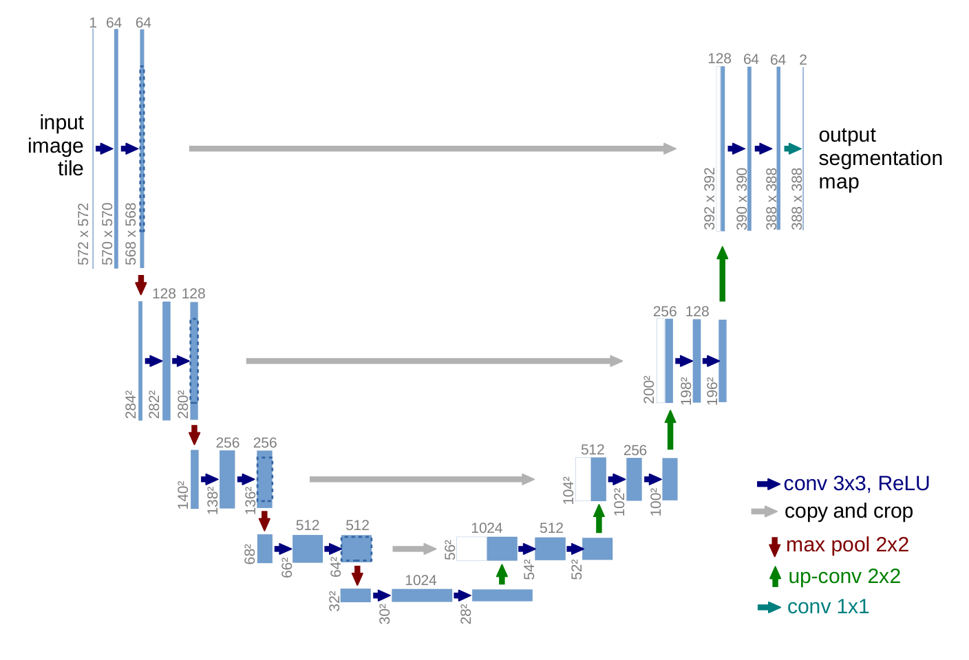
Figure source: [14], arXiv:1505.04597v1, PDF page 2. Original PDF.
Method
Build on a fully convolutional network [13] and make it symmetric.
- The contracting path repeats two 3×3 convolutions with ReLU and a 2×2 max pooling, doubling the channels at each step.
- The expanding path upsamples, applies a 2×2 “up-convolution” that halves the channels, concatenates the cropped feature map from the same level of the contracting path, and applies two 3×3 convolutions. The concatenation hands fine spatial detail to the layers that decide the label. The paper does not use the phrase “skip connection”; its figure calls this “copy and crop”.
- All convolutions are unpadded (“valid”), so the output is smaller than the input. Large images are cut into overlapping tiles (the overlap-tile strategy), and missing context at the image border is filled by mirroring.
The shrinkage is easy to compute. A 3×3 valid convolution removes 2 pixels from each dimension, and pooling needs an even size:
Code · Python · 13 lines
def unet_output_size(n, depth=4):
    """Output size of a U-Net with valid 3x3 convs, 2x2 pooling and 2x2 up-convs."""
    for _ in range(depth):          # contracting path
        n = n - 4                   # two valid 3x3 convs lose 2 pixels each
        assert n % 2 == 0, "max-pool needs an even size"
        n //= 2
    n = n - 4                       # bottom of the U: two valid convs
    for _ in range(depth):          # expanding path
        n = n * 2 - 4               # up-conv doubles, two valid convs lose 4
    return n

print(unet_output_size(572))                # 388
print((572 - unet_output_size(572)) // 2)   # 92
A 572×572 input tile, the size drawn in the paper’s Figure 1, gives a 388×388 output, so each side of the tile only supplies 92 pixels of context.
Weighted loss for touching cells. The loss is a per-pixel softmax cross-entropy with a weight map :
Here is the set of pixel positions, is the predicted probability of the true class at pixel , balances class frequencies, and , are the distances from to the border of the nearest and the second-nearest cell. The exponential term is large only in thin gaps between two cells, where is small. The paper sets and pixels (its Section 3). The printed Equation (1) has no minus sign; the sign above is the usual convention for a loss to be minimized.
Elastic deformation. Random displacement vectors are drawn on a coarse 3×3 grid from a Gaussian with a standard deviation of 10 pixels, then interpolated bicubically to every pixel (Section 3.1). The authors say this “seems to be the key concept” for training with few images.
Results
The first test is the EM neuronal-structure segmentation challenge of ISBI 2012 [21] (30 training images of 512×512 pixels), which the paper says is scored with warping, Rand and pixel error. In Table 1 (a challenge snapshot dated March 6th, 2015, sorted by warping error) U-Net, averaged over 7 rotated versions of the input, has a warping error of 0.000353, against 0.000420 for the sliding-window network. In Table 2, on two 2D light-microscopy datasets of the cell tracking challenge [22], the IOU is 0.9203 on PhC-U373 (35 partially annotated training images) and 0.7756 on DIC-HeLa (20 images), against 0.83 and 0.46 for the second-best 2015 entry. Training took about 10 hours on one GPU.
Reading the evidence
- Table 1 is a leaderboard, not an experiment. The test labels are secret and the organizers score the submission. U-Net leads the warping error by a hair: 0.000353 against 0.000355 for the runner-up, and the paper gives no repeat runs or spread. On Rand error the table itself shows entries ahead of U-Net, and the text says the better ones apply highly dataset-specific post-processing to the earlier network’s probability map; a footnote says the authors of that algorithm submitted 78 different solutions. Check which metric the headline uses and how much a “rank 1” is worth.
- Averaging over 7 rotated inputs is test-time augmentation. Ask whether the baselines got the same.
- Table 2 mixes sources. The competitor rows come from the challenge, not from reruns by the authors, and “second-best 2015” is rounded to two digits. The paper does not say whether the competing entries trained on the same images.
Problems
The paper contains no ablation: nothing removes the weighted loss, the elastic deformation or the concatenation to measure their separate effect, so the “key concept” remark is the authors’ belief, not a result. All three datasets are small 2D microscopy sets, and no repeat runs or spread are reported. Whether the same recipe works for other image types, or in 3D, is not tested here.
Conclusion
In this tutorial U-Net is the learned counterpart of two classical ideas: multi-scale analysis (the contracting path) and exact boundary placement from fine data (the concatenated high-resolution features). The same encoder–decoder with same-level connections became a standard backbone well beyond segmentation; for restoration, see DLCV 04 · Deep Image Restoration.
References
- R. C. Gonzalez and R. E. Woods, Digital Image Processing, 4th ed., Pearson, 2018, Ch. 10. publisher page
- D. Marr and E. Hildreth, “Theory of edge detection,” Proceedings of the Royal Society of London. Series B, vol. 207, no. 1167, pp. 187–217, 1980. doi
- J. Canny, “A Computational Approach to Edge Detection,” IEEE Transactions on Pattern Analysis and Machine Intelligence, vol. PAMI-8, no. 6, pp. 679–698, 1986. doi
- R. O. Duda and P. E. Hart, “Use of the Hough transformation to detect lines and curves in pictures,” Communications of the ACM, vol. 15, pp. 11–15, 1972. doi
- N. Otsu, “A Threshold Selection Method from Gray-Level Histograms,” IEEE Transactions on Systems, Man, and Cybernetics, vol. 9, no. 1, pp. 62–66, 1979. doi
- M. Sezgin and B. Sankur, “Survey over image thresholding techniques and quantitative performance evaluation,” Journal of Electronic Imaging, vol. 13, no. 1, pp. 146–165, 2004. doi
- J. Sauvola and M. Pietikäinen, “Adaptive document image binarization,” Pattern Recognition, vol. 33, no. 2, pp. 225–236, 2000. doi
- R. Achanta, A. Shaji, K. Smith, A. Lucchi, P. Fua and S. Süsstrunk, “SLIC Superpixels Compared to State-of-the-Art Superpixel Methods,” IEEE Transactions on Pattern Analysis and Machine Intelligence, vol. 34, no. 11, pp. 2274–2282, 2012. doi
- J. Shi and J. Malik, “Normalized cuts and image segmentation,” IEEE Transactions on Pattern Analysis and Machine Intelligence, vol. 22, no. 8, pp. 888–905, 2000. doi
- L. Vincent and P. Soille, “Watersheds in digital spaces: an efficient algorithm based on immersion simulations,” IEEE Transactions on Pattern Analysis and Machine Intelligence, vol. 13, no. 6, pp. 583–598, 1991. doi
- S. Minaee, Y. Boykov, F. Porikli, A. Plaza, N. Kehtarnavaz and D. Terzopoulos, “Image Segmentation Using Deep Learning: A Survey,” IEEE Transactions on Pattern Analysis and Machine Intelligence, vol. 44, no. 7, pp. 3523–3542, 2022. doi · arXiv
- T. Zhou, W. Xia, F. Zhang, B. Chang, W. Wang, Y. Yuan, E. Konukoglu and D. Cremers, “Image Segmentation in Foundation Model Era: A Survey,” arXiv:2408.12957, 2024. arXiv
- J. Long, E. Shelhamer and T. Darrell, “Fully Convolutional Networks for Semantic Segmentation,” arXiv:1411.4038, 2014. arXiv
- O. Ronneberger, P. Fischer and T. Brox, “U-Net: Convolutional Networks for Biomedical Image Segmentation,” in Medical Image Computing and Computer-Assisted Intervention – MICCAI 2015, Lecture Notes in Computer Science, vol. 9351, pp. 234–241, Springer, 2015. doi · arXiv
- K. He, G. Gkioxari, P. Dollár and R. Girshick, “Mask R-CNN,” arXiv:1703.06870, 2017. arXiv
- L.-C. Chen, G. Papandreou, I. Kokkinos, K. Murphy and A. L. Yuille, “DeepLab: Semantic Image Segmentation with Deep Convolutional Nets, Atrous Convolution, and Fully Connected CRFs,” IEEE Transactions on Pattern Analysis and Machine Intelligence, vol. 40, no. 4, pp. 834–848, 2018. doi · arXiv
- A. Kirillov, E. Mintun, N. Ravi et al., “Segment Anything,” arXiv:2304.02643, 2023. arXiv
- R. Sun, T. Lei, Q. Chen, Z. Wang, X. Du, W. Zhao and A. K. Nandi, “Survey of Image Edge Detection,” Frontiers in Signal Processing, 2022. doi
- S. Xie and Z. Tu, “Holistically-Nested Edge Detection,” arXiv:1504.06375, 2015. arXiv
- D. Stutz, A. Hermans and B. Leibe, “Superpixels: An Evaluation of the State-of-the-Art,” Computer Vision and Image Understanding, vol. 166, pp. 1–27, 2018. doi
- I. Arganda-Carreras, S. C. Turaga, D. R. Berger et al., “Crowdsourcing the creation of image segmentation algorithms for connectomics,” Frontiers in Neuroanatomy, vol. 9, 2015. doi
- M. Maška, V. Ulman, D. Svoboda et al., “A benchmark for comparison of cell tracking algorithms,” Bioinformatics, vol. 30, no. 11, pp. 1609–1617, 2014. doi · Cell Tracking Challenge