DLCV 09A.3 · Video Super-Resolution: Using Time to Recover Detail
Needs: DLCV 09 · Deep Image Restoration: Low-Level Vision, DLCV 09A · Non-Blind Image Super-Resolution
Navigate: this page and this track: Navigate: this page and this track
On this page
- What you’ll learn1 min
- The big picture1 min
- Why video is not just many images2 min
- The video degradation model4 min
- Motion: optical flow and warping4 min
- Alignment strategies4 min
- Architectures by temporal design5 min
- Real-world video and compression2 min
- Training a VSR model1 min
- Evaluation5 min
- Efficiency and streaming1 min
- Failure modes1 min
- Modern view2 min
- Key takeaways1 min
- Exercises3 min
- Supplementary notes
- Paper guides
- References
Deep Learning for Computer Vision
Explore this chapter 1 interactive experiment
Keep every s-th pixel and fewer gray levels of a real photo and of a synthetic zone plate, and see false patterns (aliasing) appear unless you filter first.
What you’ll learn
- Explain how neighboring frames add measurements and temporal constraints.
- Model motion, blur, downsampling, noise and compression across frames.
- Compare flow warping, deformable alignment and attention.
- Choose windowed, recurrent or bidirectional processing under latency and memory limits.
- Evaluate spatial fidelity, temporal stability and generative artifacts together.
The big picture
A video is a stack of photos taken a fraction of a second apart. Each photo is small and a bit blurry, but the camera or the objects move a little between shots. Video super-resolution turns such a clip into a sharper, larger clip by combining what all the nearby frames saw.
Why it matters: most of the pixels people look at are video. Streams drop to low resolution when bandwidth is short, old films and home videos were recorded at low resolution, and phones, surveillance cameras, satellites and microscopes record small, noisy image sequences. A good VSR model makes these sharper without the frame-to-frame shimmering of a frame-by-frame image model. VSR is also where ideas now common in video models were developed: flow-based feature alignment, deformable alignment, long-range recurrent propagation and video transformers.
This chapter builds on DLCV 09, which covers the degradation model, training on synthetic pairs, losses and the generic image metrics; we link to it instead of repeating it. Single-image super-resolution, the setting of one frame in and one frame out, is covered in DLCV 09A. Here we focus on what time adds.
Why video is not just many images
Plain version. Independent frame upscaling misses neighboring measurements and does not enforce stable detail across time.
Sub-pixel motion gives new information
Suppose a camera samples a scene on a coarse grid of pixels. In one frame, details that fall between the sampling points are lost (or worse, folded into wrong, low-frequency patterns, which is called aliasing). If the scene shifts by a quarter of a pixel in the next frame, the same grid now samples the scene at different places. Four frames shifted by of a pixel together sample the scene four times more densely than any one of them (Figure 1, in one dimension; in two dimensions, a factor needs distinct shifts). This is the basic reason multi-frame super-resolution can beat single-image super-resolution: the extra frames are new measurements, not copies [1].
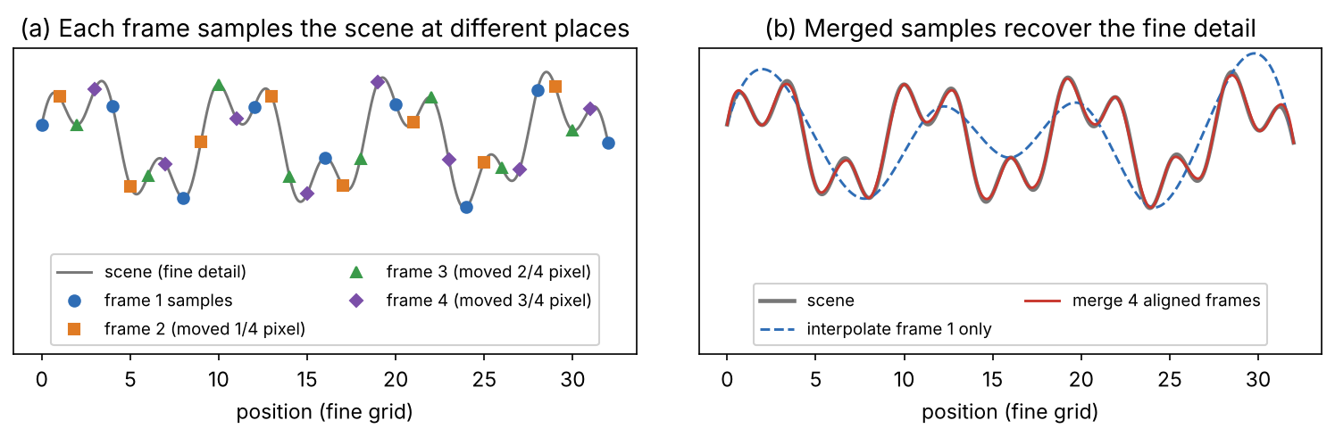
Two conditions must hold. First, the motion must be sub-pixel: a shift by a whole number of low-resolution pixels samples the same places again and adds only noise averaging. Second, we must know the motion accurately enough to put each sample in the right place. Real motion is not a global shift: objects move differently, rotate, deform, appear and disappear. Estimating and compensating that motion is the core problem of VSR, and most of this chapter is about it.
Temporal redundancy
Consecutive frames are also highly redundant: most of the scene is seen again. Independent noise averages out over repeated views, and a model can reuse work done for earlier frames. Video codecs exploit the same redundancy by predicting each frame from the previous one with motion vectors (see the motion-compensated prediction in IP 08).
Temporal consistency and flicker
A single-image model, applied frame by frame, makes small independent decisions in every frame. Where it invents texture (grass, hair, water, noise-like detail), the invented texture differs from frame to frame, and the video flickers or “boils”. Such temporal artifacts are visible even when each frame looks fine on its own. VESPCN [2] and FRVSR [3] both list temporal consistency as a main motivation for processing frames jointly instead of independently. So a VSR model has two goals: each frame should be faithful and sharp, and consecutive frames should change only as the scene changes.
The video degradation model
Plain version. Each low-resolution frame is the high-resolution frame at that moment, blurred, shrunk, made noisy and usually compressed. The frames differ because the scene moved.
One equation per frame
Extending the super-resolution model of DLCV 09 to a clip of high-resolution (HR) frames gives
where is the low-resolution (LR) frame at time , a blur kernel (camera optics, sensor integration, anti-aliasing filter), 2-D convolution, keeps every -th pixel in each direction ( is the scale factor, usually 4 in benchmarks), noise that is new in every frame, and lossy video compression (the identity in clean benchmarks). Motion enters because each is a moved version of its neighbors. Near frame we can write
where is the motion (warping) from frame to frame , is a small frame offset, and hides what motion cannot explain: occluded regions, objects entering the frame, lighting changes. Combining the two equations,
so every neighboring LR frame is a different measurement of the same unknown . VSR estimates from (a window of frames) or from the whole clip.
Multi-frame reconstruction as an inverse problem
If the motions, blur and scale were all known and there were no compression, could be found by least squares:
where is blurring with , is the downsampling , and the sum runs over the frames in the window. With one frame this problem is badly underdetermined ( unknown HR pixels per LR pixel for ). With many frames at different sub-pixel positions it becomes much better determined. Gradient descent on this objective repeatedly simulates the LR frames from the current estimate, compares them with the observed frames and spreads the error back onto the HR grid; this is the classical iterative back-projection idea introduced by Irani and Peleg [4], [1], which also inspired the RBPN architecture discussed later [5].
Optional: Classical multi-frame super-resolution (in the Supplementary notes). Fusing registered samples on the fine grid, robust (median) fusion, and when the multi-frame problem is well posed.
A toy experiment: what alignment buys
The snippet builds a 16-frame LR video from one skimage photo by random sub-pixel camera shifts, Gaussian blur, subsampling and noise. It then compares four reconstructions of the first frame: cubic interpolation of that frame alone; the average of all upsampled frames without alignment; the least-squares solver above using only the first frame; and the same solver using all 16 frames with the true shifts and with shifts estimated from the LR frames by sub-pixel phase correlation [6]. It runs in about ten seconds on a laptop CPU.
Code · Python · 49 lines
import numpy as np
from scipy import ndimage as ndi
from skimage import data, color
from skimage.registration import phase_cross_correlation

rng = np.random.default_rng(0)
s, T, blur, noise = 4, 16, 1.2, 0.01                       # scale, frames, blur sigma (HR px), noise std
hr = color.rgb2gray(data.astronaut())[64:320, 128:384]     # 256 x 256 ground-truth frame, values in [0, 1]
shifts = rng.uniform(0, s, size=(T, 2)); shifts[0] = 0     # sub-pixel camera motion of each frame (HR px)

def degrade(x, d):                                         # y_t = D B W_t x : shift, blur, keep every s-th pixel
    return ndi.gaussian_filter(ndi.shift(x, d, order=3, mode="reflect"), blur)[::s, ::s]
def degrade_T(r, d):                                       # adjoint: zero-fill, blur, shift back
    z = np.zeros((r.shape[0] * s, r.shape[1] * s)); z[::s, ::s] = r
    return ndi.shift(ndi.gaussian_filter(z, blur), -d, order=3, mode="reflect")
def upsample(y):                                           # cubic-spline interpolation on the HR grid
    u, v = np.mgrid[0:y.shape[0] * s, 0:y.shape[1] * s] / s
    return ndi.map_coordinates(y, [u, v], order=3, mode="nearest")
def psnr(x):
    c = (slice(8, -8), slice(8, -8))                       # skip a border, as benchmarks do
    return 10 * np.log10(1 / np.mean((np.clip(x, 0, 1)[c] - hr[c]) ** 2))

lr = np.stack([degrade(hr, d) + noise * rng.standard_normal((64, 64)) for d in shifts])
print("LR video:", lr.shape)

def reconstruct(frames, ds, iters=20):
    """Multi-frame least squares by gradient descent (iterative back-projection)."""
    x = np.mean([ndi.shift(upsample(f), -d, order=3, mode="reflect") for f, d in zip(frames, ds)], 0)
    for _ in range(iters):
        grad = np.mean([degrade_T(degrade(x, d) - f, d) for f, d in zip(frames, ds)], 0)
        x -= s * s * grad
    return x

# shifts estimated from the LR frames themselves (sub-pixel phase correlation), in HR pixels
est = np.array([-s * phase_cross_correlation(lr[0], f, upsample_factor=100)[0] for f in lr])
print(f"mean shift error: {np.abs(est - shifts).mean():.2f} HR px")

print(f"single frame, cubic interpolation {psnr(upsample(lr[0])):.2f} dB")
print(f"average of frames, no alignment   {psnr(np.mean([upsample(f) for f in lr], 0)):.2f} dB")
print(f"single frame, same solver         {psnr(reconstruct(lr[:1], shifts[:1])):.2f} dB")
print(f"{T} frames, true shifts            {psnr(reconstruct(lr, shifts)):.2f} dB")
print(f"{T} frames, estimated shifts       {psnr(reconstruct(lr, est)):.2f} dB")
# LR video: (16, 64, 64)
# mean shift error: 0.13 HR px
# single frame, cubic interpolation 25.50 dB
# average of frames, no alignment   20.99 dB
# single frame, same solver         25.81 dB
# 16 frames, true shifts            30.30 dB
# 16 frames, estimated shifts       29.33 dB
Three lessons from this toy run (all numbers are from our run, not from any paper). First, averaging without alignment is worse than using one frame (20.99 against 25.50 dB): misaligned frames smear the image, exactly the “forgot how far you moved” failure of the analogy. Second, the gain comes from the frames, not the solver: the same least-squares solver on one frame barely beats interpolation (25.81 dB), while 16 frames give 30.30 dB. Third, the motion can be estimated from the LR frames themselves with an average error of about an eighth of an HR pixel, which keeps most of the gain (29.33 dB). Figure 2 shows the crops and how PSNR grows with the number of frames.
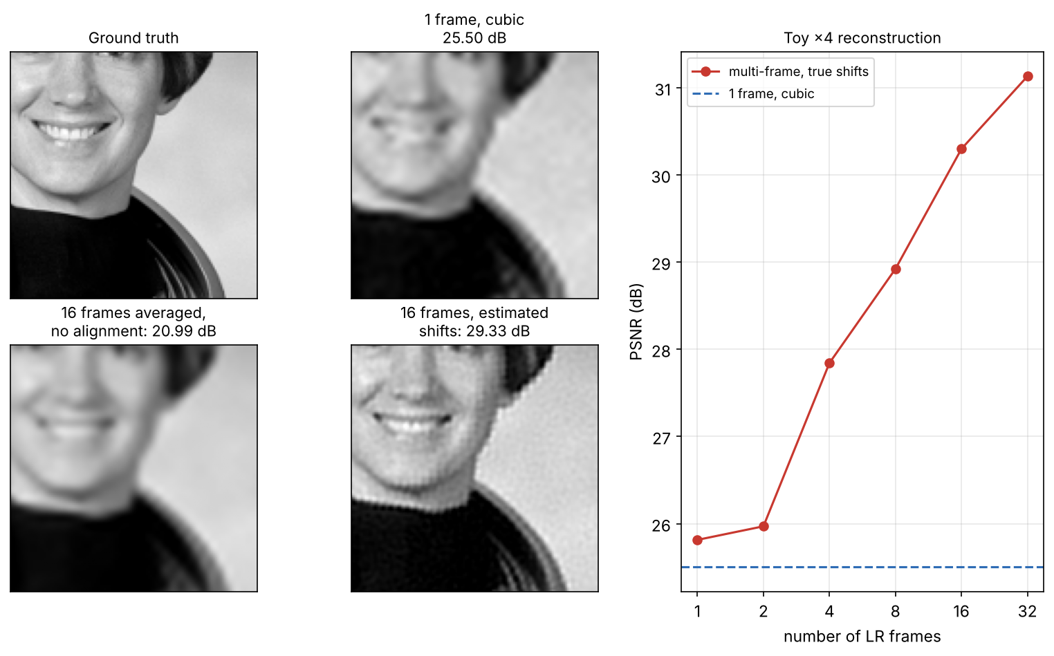
Drag the slider to compare single-frame interpolation with the 16-frame reconstruction on an enlarged crop.

 1 frame, cubic16 frames, estimated shifts
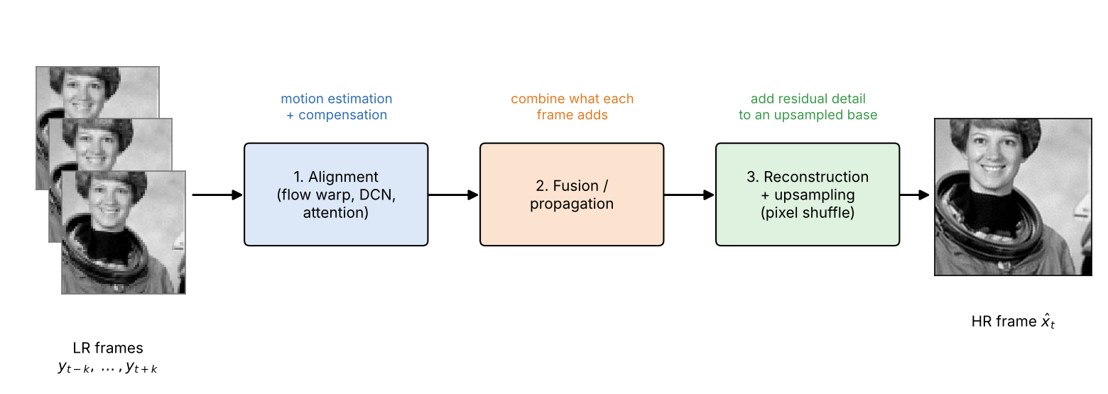
Real videos break the toy’s assumptions (global shifts, known blur, no occlusion or compression). Deep VSR keeps the structure (estimate motion, align, fuse, reconstruct) and learns each part from data. Figure 3 shows the pipeline that almost every method follows in some form; BasicVSR [7] names its four components propagation, alignment, aggregation and upsampling.
Motion: optical flow and warping
Plain version. Optical flow estimates pixel correspondences between frames. Warping resamples a frame using those correspondences to align its content.
Optical flow
The classical starting point is brightness constancy: a point keeps its brightness as it moves,
where is the intensity at column , row and time , and is the displacement of that point between frames and . The field of displacements over all pixels is the optical flow for each pixel . One equation per pixel cannot determine two unknowns (the “aperture problem”: along a straight edge only the motion across the edge is visible), so every method adds an assumption that neighboring pixels move similarly. Horn and Schunck [8] add a global smoothness penalty; Farnebäck’s method [9], available in OpenCV, fits a quadratic polynomial to each neighborhood and estimates the displacement from how the polynomial moves.
Deep flow estimators learn this mapping from data. SPyNet [10] estimates large motions coarse to fine: at each level of an image pyramid it warps one image by the current flow and a small network predicts the remaining, small update; it is compact and is the flow module of BasicVSR [7]. RAFT [11] builds correlation volumes between all pairs of pixels and refines a flow field iteratively with a recurrent unit. BasicVSR, for example, starts from a pretrained SPyNet and fine-tunes it together with the rest of the model [7].
Optional: Brightness constancy and the classical flow solvers (in the Supplementary notes). The linearized flow equation, the aperture problem, and what global (Horn–Schunck), local-window and polynomial-expansion (Farnebäck) solvers add.
Backward warping with bilinear sampling
To align frame to frame , we use the flow from to and pull values: for every pixel of the reference frame, look up where that point is in the other frame and read the value there,
where is frame warped into the coordinates of frame and is the displacement of pixel . This is backward warping: every output pixel gets exactly one value, with no holes. (Forward warping, pushing each source pixel to its new place, leaves holes and collisions.) The position is usually not on the pixel grid, so the value is interpolated bilinearly from the four surrounding pixels:
where with integer and fractions , and is the value at . Bilinear sampling is differentiable with respect to both the image values and the flow, so a network can learn the flow end to end through the warp; this “bilinear sampler” is the core of spatial transformer networks [12] and of every flow-based VSR model.
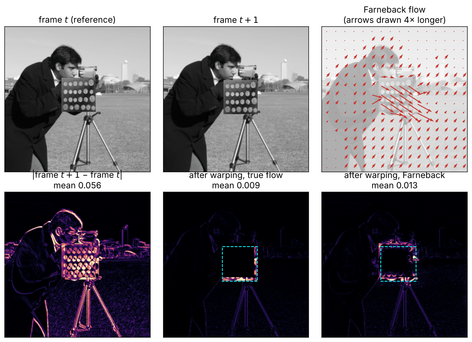
The snippet below implements backward warping by hand, checks it against cv2.remap, builds two frames in which the background moves by pixels and a textured square moves by pixels, and warps the second frame onto the first with the true flow and with Farnebäck flow from OpenCV.
Code · Python · 49 lines
import numpy as np, cv2
from scipy import ndimage as ndi
from skimage import data, transform

def bilinear_warp(img, flow):
    """Backward warping: out(p) = img(p + flow(p)), bilinear sampling. flow[..., 0] = dx, flow[..., 1] = dy."""
    H, W = img.shape
    yy, xx = np.mgrid[0:H, 0:W].astype(np.float64)
    x = np.clip(xx + flow[..., 0], 0, W - 1); y = np.clip(yy + flow[..., 1], 0, H - 1)
    x0 = np.minimum(np.floor(x).astype(int), W - 2); y0 = np.minimum(np.floor(y).astype(int), H - 2)
    ax, ay = x - x0, y - y0                                   # fractional parts = bilinear weights
    return ((1 - ay) * ((1 - ax) * img[y0, x0] + ax * img[y0, x0 + 1])
            + ay * ((1 - ax) * img[y0 + 1, x0] + ax * img[y0 + 1, x0 + 1]))

# two frames: the background moves by (dx, dy) = (1.5, -2.0) px, a textured square moves by (6, 4) px
bg = transform.resize(data.camera() / 255.0, (256, 256), anti_aliasing=True)
obj = transform.resize(data.coins() / 255.0, (60, 60), anti_aliasing=True)
def frame(t):
    f = ndi.shift(bg, (-2.0 * t, 1.5 * t), order=3, mode="reflect")   # ndi.shift takes (rows, cols)
    r, c = 90 + 4 * t, 100 + 6 * t
    f[r:r + 60, c:c + 60] = obj
    return f
I0, I1 = frame(0).astype(np.float32), frame(1).astype(np.float32)

# true backward flow from frame 0 to frame 1: where is pixel p of frame 0 found in frame 1?
flow = np.zeros((256, 256, 2), np.float32); flow[..., 0], flow[..., 1] = 1.5, -2.0
flow[90:150, 100:160] = (6.0, 4.0)
mine = bilinear_warp(I1, flow)
H, W = I0.shape; yy, xx = np.mgrid[0:H, 0:W].astype(np.float32)
ocv = cv2.remap(I1, xx + flow[..., 0], yy + flow[..., 1], cv2.INTER_LINEAR, borderMode=cv2.BORDER_REPLICATE)
print(f"max |ours - cv2.remap| = {np.abs(mine - ocv)[5:-5, 5:-5].max():.4f}")

u8 = lambda a: (np.clip(a, 0, 1) * 255).round().astype(np.uint8)        # Farneback expects 8-bit images
est = cv2.calcOpticalFlowFarneback(u8(I0), u8(I1), None, pyr_scale=0.5, levels=4, winsize=21,
                                   iterations=5, poly_n=7, poly_sigma=1.5, flags=0)
m0 = np.zeros((H, W), np.float32); m0[90:150, 100:160] = 1          # square in frame 0
m1 = np.zeros((H, W), np.float32); m1[94:154, 106:166] = 1          # square in frame 1
occl = (bilinear_warp(m1, flow) > 0) & (m0 == 0)                  # background of frame 0 hidden in frame 1
inner = (slice(8, -8), slice(8, -8))
for name, img in [("no alignment", I1), ("warped, true flow", mine), ("warped, Farneback", bilinear_warp(I1, est))]:
    e = np.abs(img - I0)
    print(f"{name:18s} mean |error| {e[inner].mean():.4f}   on occluded pixels {e[occl].mean():.4f}")
print("Farneback median flow (dx, dy): square", np.median(est[100:140, 110:150], axis=(0, 1)).round(2),
      " background", np.median(est[200:240, 20:60], axis=(0, 1)).round(2))
# max |ours - cv2.remap| = 0.0000
# no alignment       mean |error| 0.0562   on occluded pixels 0.2367
# warped, true flow  mean |error| 0.0089   on occluded pixels 0.2617
# warped, Farneback  mean |error| 0.0133   on occluded pixels 0.1733
# Farneback median flow (dx, dy): square [6. 4.]  background [ 1.42 -1.88]
Warping with the true flow cuts the mean difference between the frames by a factor of about six, and Farnebäck’s estimate gets most of the way there (our run). But look at the occluded pixels: the strip of background that the square covers in frame . There, even the true flow gives a large error, because the content simply is not in frame ; it is hidden behind the square. No flow can fix that. A VSR model must learn to trust the warped frame where it is consistent and to ignore it where it is not (Figure 4).
Alignment strategies
Plain version. Alignment can use explicit flow, learned deformable sampling locations or attention to corresponding content.
Explicit alignment: flow-based warping
The direct approach estimates a flow from each neighbor to the reference frame and warps the neighbor with it.
- VESPCN [2] (CVPR 2017) trains a fast multi-resolution spatial-transformer motion-compensation module end to end with a spatio-temporal version of the sub-pixel convolution (pixel shuffle) network ESPCN [13].
- TOFlow [14] (IJCV 2019) trains the flow network jointly with the restoration network, so the flow is task-oriented: it moves whatever makes the output best, even where that differs from physical motion. The paper also introduced Vimeo-90K.
- Image versus feature warping. Early methods warp the LR images. Inaccurate flow then produces blurry or wrong warped images, and the loss of detail cannot be undone later. Later methods compute flow on images but warp feature maps, so subsequent layers can correct small misalignments; the BasicVSR ablation found feature warping better than image warping [7].
Flow-based alignment is interpretable and works well for moderate motion. Its weaknesses are the cost of the flow network, errors at occlusions and motion boundaries, and the fact that one flow vector per pixel can point to only one place.
Implicit alignment: deformable convolution
A normal convolution reads its input on a fixed grid around each pixel. A deformable convolution [15] adds a learned offset to each of the sampling positions:
where is the output at pixel , the number of kernel taps (9 for ), the weight of tap , its fixed grid position (for example ), a learned, real-valued offset predicted by a small network for every pixel and tap, and is read with bilinear sampling. DCNv2 [16] also multiplies each tap by a learned modulation weight in , which lets the layer down-weight unreliable positions.
For alignment, the offsets are predicted from the features of the reference frame and a neighbor, and the deformable convolution is applied to the neighbor’s features. TDAN [17] aligns each supporting frame to the reference this way at the feature level without computing optical flow. EDVR [18] applies deformable alignment in a Pyramid, Cascading and Deformable (PCD) module, coarse to fine over a feature pyramid to handle large motions, and fuses the aligned features with temporal and spatial attention (TSA); it won all four tracks of the NTIRE 2019 video restoration challenges.
Chan et al. [19] showed that a deformable convolution can be decomposed into several spatial warps (one per kernel tap, each with its own offset field) followed by a convolution. So deformable alignment is a generalization of flow warping with several flow fields instead of one; this offset diversity is why it aligns better. The same work, and BasicVSR++ [20], report that deformable alignment is unstable to train: offsets can grow very large (“offset overflow”). BasicVSR++ therefore predicts the deformable offsets as a residual on top of optical flow (flow-guided deformable alignment), combining the stability of flow with the diversity of deformable sampling.
Optional: Deformable convolution as warping plus convolution (in the Supplementary notes). The decomposition in two lines, a tested example, and why several offset fields help at occlusions.
Alignment without an explicit motion step
Some models skip motion estimation altogether and let the network absorb motion. DUF [21] predicts, for every output pixel, a dynamic upsampling filter and a residual from a spatio-temporal neighborhood of the input frames, so motion is handled implicitly by the content-dependent filters. PFNL [22] fuses frames progressively and uses a non-local operation, which compares every position with every other, instead of motion estimation and compensation. 3-D convolutions over (time, height, width) are a third option. These methods avoid flow errors, but their effective search range is bounded by the receptive field, so large motions are harder.
Attention and transformers
Attention lets each position compare itself with many candidate positions in other frames and take a weighted average of the best matches, which is a soft, learned version of motion search. VRT [23] divides the video into short clips and uses temporal mutual self-attention (TMSA): mutual attention between two frames performs joint motion estimation, alignment and fusion, while self-attention extracts features; the clip partition shifts in alternate layers so information crosses clip borders, and a parallel warping module adds flow-based warping of neighboring features. VRT is applied to video SR, deblurring, denoising, frame interpolation and space-time SR. RVRT [24] uses guided deformable attention: starting from optical flow, it predicts several relevant locations in the previous clip and aggregates their features with attention weights.
Architectures by temporal design
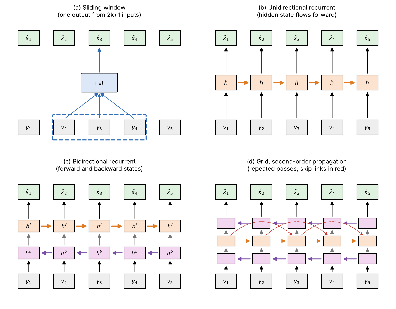
Plain version. Once frames can be aligned, the question is which frames each output gets to see, and how information travels along the video. There are four main answers, shown in Figure 5.
Sliding window
A sliding-window model takes consecutive LR frames and produces one HR frame, the center one, then moves the window by one frame. VESPCN, DUF, TDAN and EDVR are sliding-window models. It is simple and parallel, and errors cannot accumulate over time. FRVSR [3] points out two weaknesses: each input frame is processed and warped times, and each output is estimated independently, which limits temporal consistency. A fixed window also cannot use information from farther away; the BasicVSR authors measured that cutting the test sequences into shorter independent segments lowers PSNR, most strongly at segment ends [7].
Recurrent
A recurrent model keeps a hidden state that summarizes the past and updates it frame by frame:
where is a network that combines the current LR frame with the previous state warped to frame by the flow (the warp is the backward warping of the previous section), and is the reconstruction and upsampling head. Because the state is aligned before reuse, information can travel over many frames at a fixed cost per frame. (For recurrent networks in general, see ML 04.) FRVSR [3] feeds the previous HR output, warped by flow and rearranged to LR size, into the network for the next frame, which encourages temporally consistent results and needs only one warp per step. RBPN [5] is a hybrid: within a window it integrates the neighboring frames one at a time with a recurrent encoder–decoder inspired by back-projection, feeding the estimated motion as an input instead of warping the frames.
A unidirectional recurrent model sees only the past. Early frames receive little information, and errors in the state (from a bad flow, an occlusion or a scene cut) are carried into later frames: error accumulation.
Bidirectional recurrent
BasicVSR [7] runs two recurrent branches, one forward and one backward in time:
where and are the backward and forward features at frame , and the two branches (each estimates flow with SPyNet between its two input frames, warps the propagated feature with it and refines it with residual blocks), and concatenates both features and upsamples them with pixel shuffle. Every output now sees the whole clip, past and future. The paper’s ablations found a clear PSNR drop for a unidirectional variant at early frames and a larger drop without alignment, which supports its recipe: bidirectional propagation plus flow-based feature alignment is enough to be a strong baseline. Its extension IconVSR adds an information-refill module that re-extracts features from sparse keyframes to limit error accumulation at occlusions and boundaries, and coupled propagation that feeds the backward branch’s output into the forward branch.
The price is latency: the backward branch needs the future frames, so the whole clip (or a long chunk) must be available before the first output. That suits offline processing and streaming with a buffer, not live video.
Optional: BasicVSR and IconVSR (in the Paper guides). What the four-component analysis showed, the ablations to look at and the limits of the setup.
Grid and second-order propagation
BasicVSR++ [20] makes propagation richer in two ways. Grid propagation passes features backward and forward several times in alternation, so each frame’s features are refined repeatedly with information from the whole sequence. Second-order connections let the state at frame use frames and (a second-order Markov chain instead of first-order), so information can bypass one bad frame, which helps at occlusions and fine structures. With the flow-guided deformable alignment described above, BasicVSR++ reports a 0.82 dB PSNR gain over BasicVSR at a similar parameter count, and it won three tracks and placed second in a fourth in the NTIRE 2021 video super-resolution and compressed video enhancement challenges [20].
Transformers and recurrent–transformer hybrids
VRT [23] processes all frames in parallel with long-range temporal attention at several scales, which is powerful but heavy. RVRT [24] describes the trade-off directly: parallel models fuse temporal information well but have a large model size and high memory use, while recurrent models share parameters across frames and are compact but are weaker at long-range modeling and harder to parallelize. RVRT processes neighboring frames as a clip in parallel inside a globally recurrent framework, using the inferred previous clip to estimate the next, with guided deformable attention for clip-to-clip alignment.
The table summarizes the representative methods of this chapter.
| Method | Venue | Temporal design | Alignment |
|---|---|---|---|
| VESPCN [2] | CVPR 2017 | sliding window | flow (spatial transformer), image level |
| FRVSR [3] | CVPR 2018 | recurrent (previous HR output) | flow, image level |
| DUF [21] | CVPR 2018 | sliding window | none (dynamic filters) |
| TOFlow [14] | IJCV 2019 | sliding window | task-oriented flow |
| EDVR [18] | CVPRW 2019 | sliding window | deformable (PCD) + attention fusion |
| RBPN [5] | CVPR 2019 | recurrent over a window | motion as input, back-projection |
| PFNL [22] | ICCV 2019 | sliding window (progressive fusion) | none (non-local) |
| TDAN [17] | CVPR 2020 | sliding window | deformable, feature level |
| BasicVSR / IconVSR [7] | CVPR 2021 | bidirectional recurrent | flow, feature level |
| BasicVSR++ [20] | CVPR 2022 | grid, second-order | flow-guided deformable |
| RVRT [24] | NeurIPS 2022 | clip-recurrent transformer | guided deformable attention |
| VRT [23] | TIP 2024 | parallel transformer | mutual attention + parallel warping |
Real-world video and compression
Plain version. Benchmark LR videos are made by one clean, known recipe. Real videos are noisy, blurred in unknown ways and, above all, compressed. A model trained on the clean recipe often sharpens the compression artifacts instead of the scene.
Compression is the main real-world degradation
Most video is stored and streamed with block-based codecs such as H.264/AVC [25], which predict each block from earlier frames with motion vectors and quantize the residual. The resulting artifacts (blocking, ringing, smeared texture, mosquito noise around edges) differ from frame to frame: frames coded without reference to others (intra frames) look different from predicted frames, and the quality changes with the bitrate. These artifacts are not independent noise and they move with the content, so a VSR model can mistake them for real detail and propagate them. COMISR [26] designs VSR for compressed input, with bidirectional recurrent warping, detail-preserving flow estimation and a Laplacian enhancement module that take compression properties such as the position of intra frames into account, and evaluates over a range of compression rates.
Real-world VSR: RealBasicVSR
RealBasicVSR [27] (CVPR 2022) found that long-term propagation, which helps for mild degradations, can exaggerate severe artifacts: noise and compression artifacts are propagated and amplified along with the useful information. Its fix is an image pre-cleaning module applied to each frame before a BasicVSR network. It also introduced VideoLQ, a set of real low-quality videos without ground truth, evaluated with no-reference metrics and visual comparison.
Optional: RealBasicVSR (in the Paper guides). The three trade-offs it identifies and how to read its experiments.
The degradation pipelines are the video versions of the blind pipelines in DLCV 09: random blur, resizing, noise and compression, with the extra choice of applying the same or different parameters to all frames of a clip.
Diffusion-based VSR
Pretrained text-to-image diffusion models produce very realistic textures for real-world image SR (see DLCV 09). In video, their randomness is a problem: independent sampling per frame produces different textures in every frame, which is flicker at its worst. Recent methods therefore add temporal machinery to a pretrained generative model: temporal layers plus flow-guided propagation of latents across the sequence (Upscale-A-Video [28], CVPR 2024), a motion-guided loss that steers the sampling path (MGLD-VSR [29], ECCV 2024), a text-to-video model that already models motion (STAR [30], ICCV 2025), a diffusion transformer for videos of arbitrary length and resolution (SeedVR [31], CVPR 2025), and one-step distillation to cut the cost (DLoRAL [32], NeurIPS 2025).
Optional: Diffusion-based VSR models (in the Supplementary notes). What each of these five models adds to a pretrained diffusion model to keep the video consistent.
These models give the most convincing textures on real videos, but they inherit the image-level risk of hallucinated detail (plausible content that was never in the scene) and add a video-level risk: detail that is plausible in each frame but not consistent across frames. They are also far more expensive than CNN or transformer VSR.
Training a VSR model
Plain version. Training is the same as for image restoration, except that each training example is a short clip, not a single image.
Pairs are made by degrading HR clips with the model above: the bicubic (BI) or blur-downsampling (BD) recipe for benchmarks (see Evaluation), or a randomized real-world pipeline. Each step samples a short clip and random crops at the same location in all frames; flips and rotations are applied identically to all frames, and the frame order can be reversed as temporal augmentation (BasicVSR reverses Vimeo-90K’s 7-frame sequences this way [7]). Recurrent models are trained on longer clips (BasicVSR’s REDS setting uses 15-frame inputs) so that propagation is exercised; RealBasicVSR’s finding that longer sequences beat larger batches points the same way [27]. In BasicVSR the pretrained flow network and feature extractor are frozen for the first 5,000 iterations, and the flow network is then trained with a smaller learning rate than the rest [7].
The loss is usually an L1-type pixel loss on every output frame (BasicVSR uses the smooth version with a small constant , where is the difference between an output and a ground-truth pixel [7]), with perceptual and adversarial terms for real-world models; DLCV 09 covers these. Some methods add a temporal loss that penalizes differences between consecutive outputs after motion compensation, such as the short-term warping loss of Lai et al. [33], which compares each output frame with the previous output warped by optical flow, masked where the warp is unreliable.
Evaluation
Plain version. Score every frame against the ground truth, average the scores, and say exactly how the LR frames were made. Then check the video in motion, because per-frame scores cannot see flicker.
Per-frame fidelity: Y-channel PSNR and SSIM
Most VSR papers report PSNR and SSIM [34] (defined in DLCV 09) on the luminance (Y) channel, computed for every frame and averaged over the frames of a clip and then over clips. The Y channel follows ITU-R BT.601 [35]: luma from gamma-corrected RGB in , quantized on the 8-bit “studio” scale as . The convention is not universal: in the BasicVSR and BasicVSR++ comparison tables, all results are computed on Y except REDS4, which is computed on RGB [7], [20]. Mixing conventions changes numbers by several dB, as the snippet shows.
Code · Python · 22 lines
import numpy as np
from skimage import data, color

def rgb_to_y(rgb):
    """BT.601 luma on the 8-bit studio scale: Y = 16 + 219 * (0.299 R + 0.587 G + 0.114 B), RGB in [0, 1]."""
    return 16 + 65.481 * rgb[..., 0] + 128.553 * rgb[..., 1] + 24.966 * rgb[..., 2]

def psnr(a, b, peak=255.0):
    return 10 * np.log10(peak ** 2 / np.mean((a.astype(np.float64) - b) ** 2))

rng = np.random.default_rng(0)
gt = np.stack([np.roll(data.astronaut(), 2 * t, axis=1) for t in range(5)]) / 255.0   # 5 ground-truth frames
out = np.clip(gt + rng.normal(0, 0.02, gt.shape) * np.array([1.0, 0.3, 1.5]), 0, 1)  # unequal error per channel

y_scores = [psnr(rgb_to_y(o), rgb_to_y(g)) for o, g in zip(out, gt)]
rgb_scores = [psnr(255 * o, 255 * g) for o, g in zip(out, gt)]
print("matches skimage rgb2ycbcr:", np.allclose(rgb_to_y(gt[0]), color.rgb2ycbcr(gt[0])[..., 0]))
print(f"Y-channel PSNR, mean of frames: {np.mean(y_scores):.2f} dB")
print(f"RGB PSNR,       mean of frames: {np.mean(rgb_scores):.2f} dB")
# matches skimage rgb2ycbcr: True
# Y-channel PSNR, mean of frames: 43.74 dB
# RGB PSNR,       mean of frames: 33.94 dB
The same output scores about 10 dB higher on Y than on RGB here (our run), partly because Y is a weighted average of the three channels, so independent channel errors partly cancel, and partly because Y spans only 219 of the 255 levels while the peak in the formula stays 255. Always state the channel, the border crop and whether the frames were rounded to 8 bits.
Degradation settings: BI and BD
Two LR recipes dominate the clean benchmarks, and results under them are not comparable:
- BI (bicubic): downsample each HR frame by with MATLAB’s
imresize, which blurs with a cubic filter and subsamples. The Vimeo-90K SR benchmark was built this way [14]. - BD (blur-downsampling): blur each HR frame with a Gaussian of standard deviation , then keep every fourth pixel, as specified in BasicVSR [7].
BD includes a stronger, known blur, so a model must deblur as well as upsample. The BasicVSR tables report REDS4 under BI only, UDM10 under BD only, and Vimeo-90K-T and Vid4 under both [7]. When you read a comparison table, check the setting of each column first.
Temporal consistency
Per-frame PSNR is blind to flicker: errors that change randomly from frame to frame can give the same average PSNR as stable errors. Three kinds of measures are used:
- Warping error [33]: warp output frame onto frame with optical flow and measure the masked difference,
where is pixel of output frame , is frame warped to frame , the number of pixels and a non-occlusion mask; the video score averages over all consecutive pairs. Its weakness: a blurry, detail-free video is very stable and scores well.
- tOF and tLP (TecoGAN [36]) compare the temporal behavior of the output with that of the ground truth instead of demanding zero change:
where and are the output and ground-truth frames, is optical flow estimated with Farnebäck’s method and is the LPIPS perceptual distance [37]. The TecoGAN authors introduced them because a plain warped-difference measure “can be easily deceived” by blurry results such as bicubic interpolation.
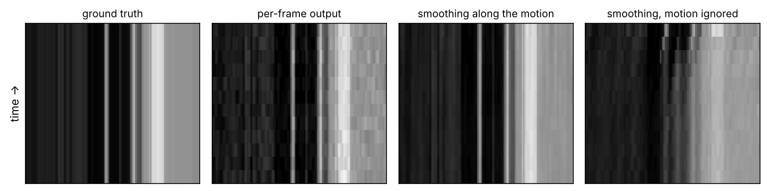
- Temporal profiles: one row of pixels followed through time and stacked into an image; speckle and streaks reveal flicker. VESPCN used them for qualitative comparison [2].
The snippet builds a toy scene with known motion and four “outputs”: independent per-frame invented texture, the same outputs smoothed recursively along the motion, the same smoothing with the motion ignored, and a blurry output. Flicker is measured in the spirit of tOF: the temporal change of the output after motion compensation, minus that of the ground truth.
Code · Python · 36 lines
import numpy as np
from scipy import ndimage as ndi
from skimage import data, transform

rng = np.random.default_rng(0)
T, v = 12, (1, 2)                                         # 12 frames, the scene moves 1 px down and 2 px right per frame
base = transform.resize(data.camera() / 255.0, (256, 256), anti_aliasing=True)
gt = np.stack([np.roll(base, (v[0] * t, v[1] * t), axis=(0, 1)) for t in range(T)])
warp_prev = lambda f: np.roll(f, v, axis=(0, 1))          # exact motion compensation for this toy scene

def fake_detail():                                        # zero-mean "hallucinated texture", new every frame
    n = ndi.gaussian_filter(rng.standard_normal(base.shape), 0.8)
    return 0.03 * n / n.std()

per_frame = gt + np.stack([fake_detail() for _ in range(T)])  # each frame restored independently
smoothed, unaligned, blurry = per_frame.copy(), per_frame.copy(), np.stack([ndi.gaussian_filter(g, 1.5) for g in gt])
for t in range(1, T):
    smoothed[t] = 0.3 * per_frame[t] + 0.7 * warp_prev(smoothed[t - 1])   # recursive filter along the motion
    unaligned[t] = 0.3 * per_frame[t] + 0.7 * unaligned[t - 1]           # same filter, motion ignored

c = (slice(None), slice(16, -16), slice(16, -16))          # ignore borders (np.roll wraps around)
def psnr(out):
    return np.mean([10 * np.log10(1 / np.mean((o - g) ** 2)) for o, g in zip(out[c], gt[c])])
def flicker(out):
    """Mean |temporal change of output - temporal change of ground truth| after motion compensation."""
    d_out = out[1:] - np.stack([warp_prev(f) for f in out[:-1]])
    d_gt = gt[1:] - np.stack([warp_prev(f) for f in gt[:-1]])
    return np.abs(d_out - d_gt)[c].mean()

for name, out in [("per-frame", per_frame), ("aligned smoothing", smoothed),
                  ("unaligned smoothing", unaligned), ("blurry output", blurry)]:
    print(f"{name:20s} PSNR {psnr(out):5.2f} dB   flicker {flicker(out):.4f}")
# per-frame            PSNR 30.50 dB   flicker 0.0338
# aligned smoothing    PSNR 36.40 dB   flicker 0.0082
# unaligned smoothing  PSNR 21.74 dB   flicker 0.0223
# blurry output        PSNR 25.99 dB   flicker 0.0000
Read the four lines together (all from our toy run). Propagating information along the motion reduces flicker and, in this toy, also improves PSNR, because the invented texture is zero-mean noise that averages out; real hallucinated texture is not, so do not expect PSNR gains of this size. Propagating without alignment ghosts the moving scene: PSNR collapses and flicker stays high. And the blurry output has zero flicker but poor PSNR, which is the TecoGAN warning in miniature: always report a temporal measure together with a fidelity or perceptual measure. Figure 6 shows the same effects as motion-compensated temporal profiles.
Datasets and test sets
| Dataset | What it is | Typical use |
|---|---|---|
| Vimeo-90K [14] | 89,800 video clips (720p or higher) from Vimeo; the SR benchmark uses 7-frame sequences at 448 × 256, with ×4 LR inputs of 112 × 64 made by MATLAB imresize | training; test split Vimeo-90K-T |
| REDS [38] | 300 sequences of 100 frames at 720 × 1280 (240 training, 30 validation, 30 test), captured for the NTIRE 2019 video challenges, with large and complex motion | training; REDS4 test set |
| REDS4 | four REDS training clips (000, 011, 015, 020) held out for testing, following EDVR [7] | test under BI |
| Vid4 [39] | four short sequences from Liu and Sun’s Bayesian adaptive VSR work | test under BI and BD |
| UDM10 | ten test sequences released with PFNL [22] | test under BD |
| VideoLQ [27] | real-world low-quality videos without ground truth | real-world evaluation (no-reference metrics, visual) |
The Liu et al. survey notes that test videos evolved from Vid4 toward REDS as methods aimed at more complex motion and scene changes [40]; BasicVSR describes REDS4 as containing large and complicated motions [7]. Because Vimeo-90K-T sequences have only seven frames, long-range propagation has little to work with there: BasicVSR reports slightly lower scores on Vimeo-90K-T than sliding-window methods such as EDVR and attributes this to the short sequences [7].
Challenges
Challenges at the NTIRE (CVPR) and AIM (ECCV) workshops created datasets and track the state of the art. NTIRE 2019 introduced REDS [38]; its video SR challenge [41] had a bicubic track and a track with realistic motion blur, and EDVR won all four video restoration tracks that year [18]. NTIRE 2021 video SR [42] had a restoration-quality track and a lower-frame-rate track, which turns the problem into space-time SR (raising resolution and frame rate together); BasicVSR++ reports three first places and one second place across that challenge and the compressed video enhancement challenge [20]. Efficiency challenges judge quality per unit of compute: the Mobile AI & AIM 2022 report [43] asked for real-time ×4 VSR on a phone’s neural processing unit, trained on REDS and judged on runtime and power, and the AIM 2024 challenge on efficient VSR for compressed content [44] targets streaming with ×4 upscaling from 540p to 4K and ×3 from 360p to 1080p.
Efficiency and streaming
Plain version. A video model must run on every frame, often in real time, and often before the future frames exist. Those constraints shape the architecture as much as accuracy does.
- Cost per frame. A sliding window processes each input frame times unless features are cached; a recurrent model processes each frame once and carries a state, so its cost per frame does not grow with the length of the video [3].
- Latency and causality. Bidirectional and grid propagation need future frames, so the first output waits for the end of the chunk. Live video (calls, game streaming) allows only causal designs or short look-ahead buffers, at some cost in quality (the unidirectional ablation of BasicVSR [7]). Long videos are processed in chunks, and quality dips at chunk ends, as BasicVSR’s segment experiment shows.
- Memory. Parallel transformers such as VRT attend across many frames at several scales; their model size and memory use are the drawback RVRT addresses with clip-level recurrence [24]. Diffusion VSR is costlier still, which motivates one-step models [32].
- Deployment. The efficiency challenges set the target for phones and streaming: few parameters and operations, real-time frame rates and low power, with quality judged against interpolation baselines rather than against the largest models [43], [44].
Failure modes
Plain version. VSR fails where its main assumption fails: that neighboring frames show the same content, slightly moved.
- Occlusion and disocclusion. Content hidden in the neighbors (Figure 4) has no extra measurements; a model that trusts the warped features there produces ghosts or doubled edges. Modulation masks and attention weights let a model down-weight such regions [20].
- Large and complex motion. Fast, non-rigid motion and motion blur make alignment inaccurate; coarse-to-fine alignment (PCD in EDVR, the pyramid in SPyNet) helps but does not remove the problem. REDS was used to stress exactly this [18].
- Error accumulation. In recurrent models a wrong state is carried forward, especially after occlusions or scene cuts; IconVSR’s keyframe refill and BasicVSR++‘s second-order links are direct countermeasures [7], [20]. Long propagation can also amplify severe input artifacts, which RealBasicVSR counters with pre-cleaning [27].
- Flicker. Independent per-frame decisions, in single-image models or in diffusion sampling, cause temporal instability that per-frame metrics cannot see.
- Hallucinated detail. GAN and diffusion VSR can create plausible texture, text or faces that were never there, and in video the invented content may also drift. For surveillance, forensic, medical or scientific video, prefer fidelity-oriented models and state which kind of model produced an output.
- Domain gap. Models trained on BI or BD degradations do not account for compression and real noise [26], [27].
Modern view
Survey papers
- Liu et al., “Video Super-Resolution Based on Deep Learning: A Comprehensive Survey” (Artificial Intelligence Review, 2022) [40]. Reviews 37 deep VSR methods in seven sub-categories by how they use inter-frame information: with alignment (motion estimation and compensation, deformable convolution) or without alignment (2-D and 3-D convolution, recurrent CNNs, non-local operations, others), and compares them on benchmarks. Takeaway: the field moved from aligned short windows toward a mix of designs and long sequences, with REDS replacing Vid4 as the demanding test set.
- Tu et al., “Optical Flow for Video Super-Resolution: A Survey” (Artificial Intelligence Review, 2022) [45]. Covers metrics and classical and deep flow-based VSR, with an analysis of representative deep methods. Takeaway: dense, sub-pixel flow is among the most common tools for motion compensation, so understanding flow is a large part of understanding VSR alignment.
- Baniya et al., “A Survey of Deep Learning Video Super-Resolution” (IEEE Transactions on Emerging Topics in Computational Intelligence, 2024) [46]. A component taxonomy (inputs, alignment, fusion, refinement and reconstruction, upsampling), plus losses, quality and efficiency evaluation, applications and trends such as online, real-world, resource-constrained and space-time VSR. Takeaway: design choices are often driven by benchmark gains rather than explained, and practical settings deserve more attention.
State of the art, 2023–2026
- Propagation plus alignment is the core of fidelity-oriented VSR. Bidirectional or grid recurrent propagation with flow-guided deformable alignment (BasicVSR++) and parallel or clip-recurrent transformers (VRT, RVRT) are the reference designs of this chapter, trading accuracy against memory and latency.
- Real-world VSR moved to generative priors. After CNN-based real-world models such as RealBasicVSR, diffusion-based VSR built on image diffusion models (Upscale-A-Video, MGLD-VSR), then on video diffusion models and diffusion transformers (STAR, SeedVR), with temporal consistency as the central technical problem.
- Cost reduction of generative VSR. One-step diffusion (DLoRAL) follows the same path as one-step image SR.
- Efficiency and compression as first-class targets, with challenge tracks for mobile hardware and compressed streaming content [43], [44].
Open problems
- Faithful versus plausible. Measuring and controlling hallucination in video, where invented detail may also be temporally unstable, is unsolved.
- Temporal evaluation. Warping error can be gamed by blur, tOF and tLP depend on flow and feature estimates, there is no agreed perceptual measure of temporal quality, and user studies are costly.
- Real degradations and codecs. Synthetic pipelines still miss real camera processing and codec behavior; ground truth for real videos is rarely available.
- Long videos, online processing and scene cuts. Combining the quality of bidirectional and global models with causal, constant-memory processing remains difficult.
- Occlusions and large motion. Alignment is still the weak point under fast, non-rigid motion and disocclusion.
- Cost of generative VSR, which is still far above that of CNN and transformer VSR for long, high-resolution video.
Key takeaways
- Sub-pixel motion can reveal extra scene measurements; independent frame upscaling discards them.
- Align corresponding content before combining it; occluded regions may have no valid match.
- Flow, deformable sampling and attention offer different correspondence mechanisms and costs.
- Recurrence propagates information and errors; bidirectional processing also needs future frames.
- Compression artifacts and generated textures can accumulate or flicker across time.
- Report the degradation, color and border protocol with spatial and temporal metrics; blur alone can look stable.
Exercises
- Integer versus sub-pixel motion. In the multi-frame snippet, replace the random shifts by integer shifts (
rng.integers(0, s, size=(T, 2)).astype(float), keepingshifts[0] = 0) and rerun. Then try all shifts equal to zero. Explain the PSNR you get in each case using the sampling argument of Figure 1.
Hint
Integer shifts in HR pixels still land the LR samples on different HR phases (an HR shift of 1 is a quarter LR pixel), so they still help; what matters is the shift modulo HR pixels. With all shifts zero every frame samples the same HR positions, so only the noise averages out and the result stays close to the single-frame solver. Try shifts that are multiples of 4 HR pixels to see the “no new information” case directly.
- Registration error budget. Add Gaussian noise with standard deviation 0.25, 0.5 and 1.0 HR pixels to the true shifts before calling
reconstruct, and plot PSNR against the shift error. Compare with the 0.13-pixel error of phase correlation. What does this suggest about how accurate alignment must be for super-resolution, compared with denoising?
Hint
PSNR should fall quickly once the shift error approaches the size of the detail being recovered (a fraction of an HR pixel), because samples land in the wrong places and the reconstruction blurs or rings. Denoising by averaging tolerates larger errors, since it only needs the same content, not its exact sub-pixel position. This is why VSR needs sub-pixel accurate flow, while many video denoisers can work with coarser alignment.
- Forward versus backward warping. Write a forward-warping function that pushes each pixel of frame to (rounded to the nearest pixel) and compare its output with
bilinear_warpon the two-frame example. Count holes (pixels that receive no value) and collisions (pixels that receive several).
Hint
Holes appear where the scene expands or is disoccluded (behind the moving square), and collisions where it contracts or is occluded. Backward warping has neither, because every output pixel reads exactly one (interpolated) value, which is why networks use it; the price is that it needs the flow defined on the reference frame.
- Sliding window versus recurrent cost. A sliding-window model with a 7-frame window runs a feature extractor on every input frame of the window and one flow network per neighbor. A bidirectional recurrent model runs one feature extractor per frame and two flow estimations per frame (one per direction). Count feature extractions and flow estimations per output frame for each design, with and without caching features between windows. Which design has lower latency for the first output of a 100-frame clip?
Hint
Without caching the window model does 7 feature extractions and 6 flow estimations per output; with caching, 1 new extraction per output but still 6 flows (each neighbor must be aligned to a new center). The bidirectional model does 1 extraction and 2 flows per frame. But its first output needs the backward pass over all 100 frames, while the window model needs only frames 1 to 4. Cost per frame favors recurrence; latency favors the window.
- Flicker metric pitfalls. In the flicker snippet, replace the zero-mean fake detail by a fixed texture pattern that moves with the scene (generate it once and roll it with the scene). Rerun and explain why the flicker measure changes while PSNR does not change much. What does this say about what tOF/tLP-style measures can and cannot detect?
Hint
A texture that moves consistently with the scene has the same temporal change as the ground truth, so the motion-compensated flicker drops to about zero, while PSNR stays roughly as low as before because the texture is still wrong. Temporal measures detect inconsistency, not incorrectness: a consistently hallucinated texture passes them. Fidelity (or perceptual) metrics and temporal metrics answer different questions.
References
- S. Farsiu, M. D. Robinson, M. Elad and P. Milanfar, “Fast and Robust Multiframe Super Resolution,” IEEE Transactions on Image Processing, vol. 13, no. 10, pp. 1327–1344, 2004. doi
- J. Caballero, C. Ledig, A. Aitken, A. Acosta, J. Totz, Z. Wang and W. Shi, “Real-Time Video Super-Resolution with Spatio-Temporal Networks and Motion Compensation,” in Proc. IEEE CVPR, 2017. CVF · arXiv
- M. S. M. Sajjadi, R. Vemulapalli and M. Brown, “Frame-Recurrent Video Super-Resolution,” in Proc. IEEE/CVF CVPR, 2018. CVF · arXiv
- M. Irani and S. Peleg, “Improving Resolution by Image Registration,” CVGIP: Graphical Models and Image Processing, vol. 53, no. 3, pp. 231–239, 1991. doi
- M. Haris, G. Shakhnarovich and N. Ukita, “Recurrent Back-Projection Network for Video Super-Resolution,” in Proc. IEEE/CVF CVPR, 2019. CVF · arXiv
- M. Guizar-Sicairos, S. T. Thurman and J. R. Fienup, “Efficient Subpixel Image Registration Algorithms,” Optics Letters, vol. 33, no. 2, p. 156, 2008. doi
- K. C. K. Chan, X. Wang, K. Yu, C. Dong and C. C. Loy, “BasicVSR: The Search for Essential Components in Video Super-Resolution and Beyond,” in Proc. IEEE/CVF CVPR, 2021. CVF · arXiv
- B. K. P. Horn and B. G. Schunck, “Determining Optical Flow,” Artificial Intelligence, vol. 17, no. 1–3, pp. 185–203, 1981. doi
- G. Farnebäck, “Two-Frame Motion Estimation Based on Polynomial Expansion,” in Image Analysis (Lecture Notes in Computer Science), pp. 363–370, Springer, 2003. doi
- A. Ranjan and M. J. Black, “Optical Flow Estimation Using a Spatial Pyramid Network,” in Proc. IEEE CVPR, 2017. CVF · arXiv
- Z. Teed and J. Deng, “RAFT: Recurrent All-Pairs Field Transforms for Optical Flow,” in Proc. ECCV (Lecture Notes in Computer Science), pp. 402–419, 2020. doi · arXiv
- M. Jaderberg, K. Simonyan, A. Zisserman and K. Kavukcuoglu, “Spatial Transformer Networks,” in Advances in Neural Information Processing Systems (NeurIPS), 2015. proceedings · arXiv
- W. Shi, J. Caballero, F. Huszár, J. Totz, A. P. Aitken, R. Bishop, D. Rueckert and Z. Wang, “Real-Time Single Image and Video Super-Resolution Using an Efficient Sub-Pixel Convolutional Neural Network,” in Proc. IEEE CVPR, 2016. arXiv
- T. Xue, B. Chen, J. Wu, D. Wei and W. T. Freeman, “Video Enhancement with Task-Oriented Flow,” International Journal of Computer Vision, vol. 127, no. 8, pp. 1106–1125, 2019. doi · arXiv
- J. Dai, H. Qi, Y. Xiong, Y. Li, G. Zhang, H. Hu and Y. Wei, “Deformable Convolutional Networks,” in Proc. IEEE ICCV, 2017. CVF · arXiv
- X. Zhu, H. Hu, S. Lin and J. Dai, “Deformable ConvNets V2: More Deformable, Better Results,” in Proc. IEEE/CVF CVPR, 2019. CVF · arXiv
- Y. Tian, Y. Zhang, Y. Fu and C. Xu, “TDAN: Temporally-Deformable Alignment Network for Video Super-Resolution,” in Proc. IEEE/CVF CVPR, 2020. CVF · arXiv
- X. Wang, K. C. K. Chan, K. Yu, C. Dong and C. C. Loy, “EDVR: Video Restoration with Enhanced Deformable Convolutional Networks,” in Proc. IEEE/CVF CVPR Workshops, 2019. CVF · arXiv
- K. C. K. Chan, X. Wang, K. Yu, C. Dong and C. C. Loy, “Understanding Deformable Alignment in Video Super-Resolution,” in Proc. AAAI Conference on Artificial Intelligence, vol. 35, no. 2, pp. 973–981, 2021. doi · arXiv
- K. C. K. Chan, S. Zhou, X. Xu and C. C. Loy, “BasicVSR++: Improving Video Super-Resolution with Enhanced Propagation and Alignment,” in Proc. IEEE/CVF CVPR, 2022. CVF · arXiv
- Y. Jo, S. W. Oh, J. Kang and S. J. Kim, “Deep Video Super-Resolution Network Using Dynamic Upsampling Filters Without Explicit Motion Compensation,” in Proc. IEEE/CVF CVPR, 2018. CVF
- P. Yi, Z. Wang, K. Jiang, J. Jiang and J. Ma, “Progressive Fusion Video Super-Resolution Network via Exploiting Non-Local Spatio-Temporal Correlations,” in Proc. IEEE/CVF ICCV, 2019. CVF · code and test data (Vid4, UDM10)
- J. Liang, J. Cao, Y. Fan, K. Zhang, R. Ranjan, Y. Li, R. Timofte and L. Van Gool, “VRT: A Video Restoration Transformer,” IEEE Transactions on Image Processing, vol. 33, pp. 2171–2182, 2024. doi · arXiv
- J. Liang, Y. Fan, X. Xiang, R. Ranjan, E. Ilg, S. Green, J. Cao, K. Zhang, R. Timofte and L. Van Gool, “Recurrent Video Restoration Transformer with Guided Deformable Attention,” in Advances in Neural Information Processing Systems (NeurIPS), vol. 35, pp. 378–393, 2022. arXiv
- T. Wiegand, G. J. Sullivan, G. Bjøntegaard and A. Luthra, “Overview of the H.264/AVC Video Coding Standard,” IEEE Transactions on Circuits and Systems for Video Technology, vol. 13, no. 7, pp. 560–576, 2003. doi
- Y. Li, P. Jin, F. Yang, C. Liu, M.-H. Yang and P. Milanfar, “COMISR: Compression-Informed Video Super-Resolution,” in Proc. IEEE/CVF ICCV, 2021. CVF · arXiv
- K. C. K. Chan, S. Zhou, X. Xu and C. C. Loy, “Investigating Tradeoffs in Real-World Video Super-Resolution,” in Proc. IEEE/CVF CVPR, 2022. CVF · arXiv
- S. Zhou, P. Yang, J. Wang, Y. Luo and C. C. Loy, “Upscale-A-Video: Temporal-Consistent Diffusion Model for Real-World Video Super-Resolution,” in Proc. IEEE/CVF CVPR, pp. 2535–2545, 2024. CVF · arXiv
- X. Yang, C. He, J. Ma and L. Zhang, “Motion-Guided Latent Diffusion for Temporally Consistent Real-World Video Super-Resolution,” in Proc. ECCV (Lecture Notes in Computer Science), pp. 224–242, 2024. doi · arXiv
- R. Xie, Y. Liu, P. Zhou, C. Zhao, J. Zhou, K. Zhang, Z. Zhang, J. Yang, Z. Yang and Y. Tai, “STAR: Spatial-Temporal Augmentation with Text-to-Video Models for Real-World Video Super-Resolution,” in Proc. IEEE/CVF ICCV, 2025. CVF · arXiv
- J. Wang, Z. Lin, M. Wei, Y. Zhao, C. Yang, C. C. Loy and L. Jiang, “SeedVR: Seeding Infinity in Diffusion Transformer Towards Generic Video Restoration,” in Proc. IEEE/CVF CVPR, 2025. CVF · arXiv
- Y. Sun, L. Sun, S. Liu, R. Wu, Z. Zhang and L. Zhang, “One-Step Diffusion for Detail-Rich and Temporally Consistent Video Super-Resolution,” in Advances in Neural Information Processing Systems (NeurIPS), vol. 38, 2025. arXiv
- W.-S. Lai, J.-B. Huang, O. Wang, E. Shechtman, E. Yumer and M.-H. Yang, “Learning Blind Video Temporal Consistency,” in Proc. ECCV, 2018. CVF · arXiv
- Z. Wang, A. C. Bovik, H. R. Sheikh and E. P. Simoncelli, “Image Quality Assessment: From Error Visibility to Structural Similarity,” IEEE Transactions on Image Processing, vol. 13, no. 4, pp. 600–612, 2004. doi
- ITU-R, “Recommendation ITU-R BT.601-7: Studio Encoding Parameters of Digital Television for Standard 4:3 and Wide-Screen 16:9 Aspect Ratios,” International Telecommunication Union, 2011. ITU
- M. Chu, Y. Xie, J. Mayer, L. Leal-Taixé and N. Thuerey, “Learning Temporal Coherence via Self-Supervision for GAN-based Video Generation,” ACM Transactions on Graphics, vol. 39, no. 4, article 75, 2020. doi · arXiv
- R. Zhang, P. Isola, A. A. Efros, E. Shechtman and O. Wang, “The Unreasonable Effectiveness of Deep Features as a Perceptual Metric,” in Proc. IEEE/CVF CVPR, 2018. CVF · arXiv
- S. Nah, S. Baik, S. Hong, G. Moon, S. Son, R. Timofte and K. M. Lee, “NTIRE 2019 Challenge on Video Deblurring and Super-Resolution: Dataset and Study,” in Proc. IEEE/CVF CVPR Workshops, 2019. CVF
- C. Liu and D. Sun, “On Bayesian Adaptive Video Super Resolution,” IEEE Transactions on Pattern Analysis and Machine Intelligence, vol. 36, no. 2, pp. 346–360, 2014. doi
- H. Liu, Z. Ruan, P. Zhao, C. Dong, F. Shang, Y. Liu, L. Yang and R. Timofte, “Video Super-Resolution Based on Deep Learning: A Comprehensive Survey,” Artificial Intelligence Review, vol. 55, no. 8, pp. 5981–6035, 2022. doi · arXiv
- S. Nah, R. Timofte, S. Gu, S. Baik, S. Hong, G. Moon, S. Son and K. M. Lee, “NTIRE 2019 Challenge on Video Super-Resolution: Methods and Results,” in Proc. IEEE/CVF CVPR Workshops, 2019. CVF
- S. Son, S. Lee, S. Nah, R. Timofte and K. M. Lee, “NTIRE 2021 Challenge on Video Super-Resolution,” in Proc. IEEE/CVF CVPR Workshops, 2021. CVF · arXiv
- A. Ignatov, R. Timofte et al., “Power Efficient Video Super-Resolution on Mobile NPUs with Deep Learning, Mobile AI & AIM 2022 Challenge: Report,” arXiv:2211.05256, 2022. arXiv
- M. V. Conde, Z. Lei, W. Li, C. Bampis, I. Katsavounidis, R. Timofte et al., “AIM 2024 Challenge on Efficient Video Super-Resolution for AV1 Compressed Content,” in Proc. ECCV Workshops (Lecture Notes in Computer Science), pp. 304–325, 2025. doi · arXiv
- Z. Tu, H. Li, W. Xie, Y. Liu, S. Zhang, B. Li and J. Yuan, “Optical Flow for Video Super-Resolution: A Survey,” Artificial Intelligence Review, vol. 55, no. 8, pp. 6505–6546, 2022. doi · arXiv
- A. A. Baniya, T.-K. Lee, P. W. Eklund and S. Aryal, “A Survey of Deep Learning Video Super-Resolution,” IEEE Transactions on Emerging Topics in Computational Intelligence, vol. 8, no. 4, pp. 2655–2676, 2024. doi · arXiv
- B. Wronski, I. Garcia-Dorado, M. Ernst, D. Kelly, M. Krainin, C.-K. Liang, M. Levoy and P. Milanfar, “Handheld Multi-Frame Super-Resolution,” ACM Transactions on Graphics, vol. 38, no. 4, 2019. doi · arXiv
Check your understanding
This tutorial has 5 exercises. Can you solve them without opening the hints?
Go to the exercises ↑Next DLCV 09B · Generative Image Restoration: Sampling a Plausible Answer · 38 min