DLCV 09C · Low-Light Image Enhancement
Needs: DLCV 09 · Deep Image Restoration: Low-Level Vision, IP 03 · Intensity Transformations and Spatial Filtering, IP 06 · Color Image Processing
Navigate: this page and this track: Navigate: this page and this track
On this page
- What you’ll learn1 min
- The big picture1 min
- Goal and difficulty3 min
- Non-deep-learning LLIE and the characteristics of low-light images8 min
- Deep-learning LLIE15 min
- Measuring efficiency honestly2 min
- Failure modes1 min
- Evaluation5 min
- Benchmark datasets2 min
- Modern view2 min
- Key takeaways1 min
- Exercises3 min
- Supplementary notes
- Paper guides
- References
- CLAHE: equalizing locally without amplifying noise
- More deep LLIE methods
- Counting resolution, arithmetic and memory
- A bilateral-grid experiment
- Implementing and checking trilinear LUTs
- Fitting and slicing a bilateral grid in detail
- Learnable LUT variants in detail
- Structural re-parameterization step by step
- Understanding no-reference low-light metrics
- Efficient network building blocks
- Banding, halos and temporal stability
- Bilateral grids and color-table mathematics
- From retouching to low light
- A lightness-order exercise
- KinD: repair reflectance while controlling illumination
- Retinex-Net: decompose, adjust and denoise
- EnlightenGAN: unpaired appearance learning with content constraints
- Zero-DCE and Zero-DCE++: learn curves without reference images
- RUAS: search the priors inside an unrolled enhancement model
- SCI: train with calibration, deploy one illumination block
- Retinexformer: illumination guides restoration
- IAT: local affine maps and a global camera-style transform
- Multinex: fuse analytic priors into a Retinex residual
- CPGA-Net: channel priors, gamma estimation and learned fusion
- CPGA-Net+: attention, BDSF and stronger variants
- HDRNet: deep bilateral learning for real-time image enhancement
- Image-adaptive 3D LUTs (Zeng et al., TPAMI 2022)
Deep Learning for Computer Vision
Explore this chapter 2 interactive experiments
Simulate a dim photo with photon and read noise, then compare more light, more digital gain and a denoiser.
What you’ll learn
- Separate tone correction from noise, detail and color restoration.
- Compare histogram, gamma, Retinex and photographic-transform approaches.
- Classify learning methods by supervision and architecture independently.
- Choose evaluation protocols that expose exposure, color and noise failures.
- Measure full-resolution cost and assess suitability for downstream tasks.
The big picture
A photo taken in the dark is not just a normal photo with the brightness turned down. The sensor collected very few photons, so the picture is dim, noisy, and often has a color cast. Low-light image enhancement aims to produce the image you would have gotten with good light: well exposed, with natural colors, clean details, and no new artifacts.
Why it matters: phones shoot in the dark every day, cars and robots must see at night, and surveillance, astronomy-like scientific imaging and medical endoscopy all fight the same physics. Low light also hurts downstream models: a detector trained on daytime photos loses accuracy at night. That makes LLIE both a picture-quality task and a robustness task for computer vision.
Related chapters. DLCV 09 supplies the restoration background. DLCV 10 combines complementary measurements from several images. Efficiency is discussed alongside every enhancement lineage here.
Goal and difficulty
Plain version. Low-light enhancement combines tone adjustment with restoration of noisy detail and color. Brightening alone does not solve both.
Precise version. Unlike image-to-image translation, which changes an image’s attributes (summer to winter, photo to painting), LLIE should keep the scene and its content exactly as they are and only undo the damage caused by insufficient light. The post [1] splits that damage into two difficulties:
- Tone enhancement. Lift the exposure, globally and locally, without crushing highlights or flattening contrast. Bright regions such as lamps must stay bright, dark regions must open up, and the ordering of brightness between regions should be preserved.
- Detail restoration. Recover texture and color that are buried in noise and quantization, while suppressing that noise rather than amplifying it.
In deep learning, detail restoration is what a network does anyway once it is trained to output a clean image, so most method design goes into the tone part (which image properties or physical model to build in) and the learning mechanism (which supervision and losses to use), rather than into a dedicated detail module.
Why it is not simple brightening
A linear gain with fails in four ways, all visible in Figure 1:
- Noise. Photon arrival is random. With few photons, the signal-to-noise ratio is low, and a gain multiplies signal and noise equally. The image gets brighter, not cleaner.
- Color cast. Low light is often colored (tungsten, sodium street lamps), and the camera’s white balance and the three color channels have different noise levels. Scaling the channels equally keeps the cast; scaling them separately may produce strange colors.
- Saturation and over-exposure. Pixels already near the top (lamps, windows, screens) clip at 1. A global gain big enough for the shadows destroys the highlights.
- Quantization. A dark 8-bit image may use only 20–40 distinct gray levels. Stretching them produces visible banding.
A model of low-light capture
It helps to have an explicit degradation model, both for understanding and for synthesizing training data. Work in linear light (values proportional to photon counts), not on gamma-encoded pixels (see IP 03 on gamma). A widely used model is the Poisson–Gaussian model of Foi et al. [2]:
where is the clean linear image, the fraction of light that reached the sensor, a scale that converts intensity to photon counts (a larger means more photons and less relative noise), a Poisson random variable modeling shot noise, and Gaussian read noise with standard deviation . The camera then applies a tone curve and quantizes. The variance of is approximately : it grows with the signal, so noise is signal-dependent, which is why “add Gaussian noise” is a poor stand-in for real low light.
Code · Python · 15 lines
import numpy as np
from skimage import data, img_as_float

rng = np.random.default_rng(0)
clean = img_as_float(data.coffee())            # H x W x 3, sRGB-encoded, in [0, 1]

def synth_low_light(x, k=0.05, peak=2000.0, read_std=8e-4, gamma=2.2):
    lin = k * x ** gamma                           # 1) less light, in linear units
    lin = rng.poisson(lin * peak) / peak           # 2) shot noise (Poisson)
    lin = lin + rng.normal(0, read_std, lin.shape) # 3) read noise (Gaussian)
    out = np.clip(lin, 0, 1) ** (1 / gamma)        # 4) re-encode for display
    return np.round(out * 255) / 255               # 5) 8-bit quantization

dark = synth_low_light(clean)
print(clean.mean(), dark.mean())                   # about 0.39 -> 0.10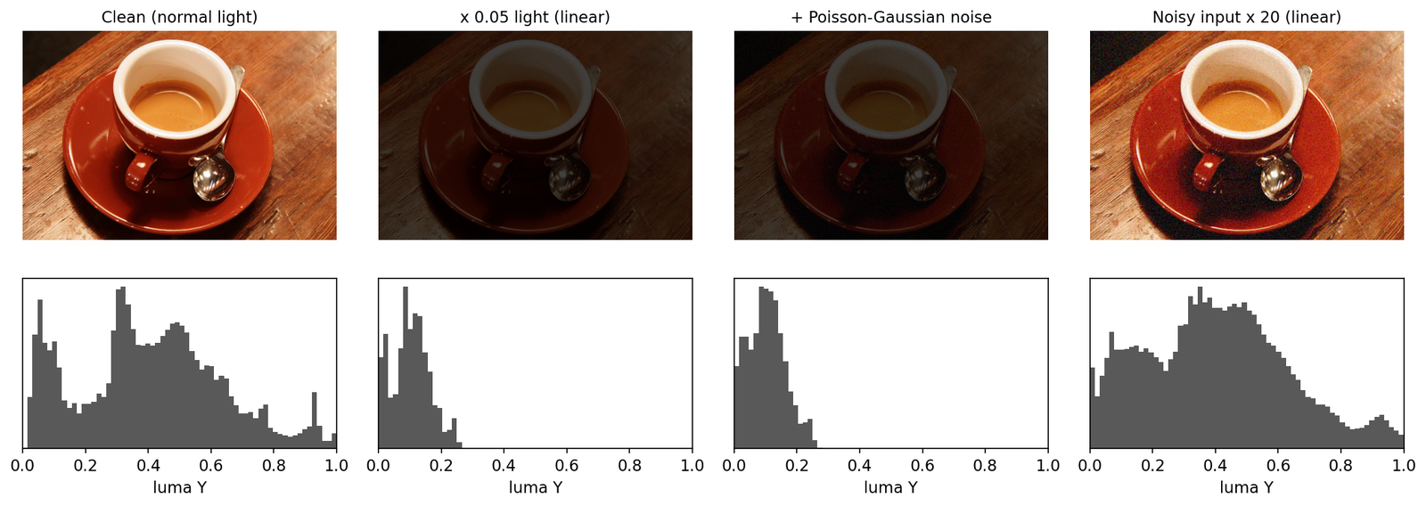
The right panel is the most important picture in this tutorial: even the ideal brightness correction leaves the noise, which is why LLIE is a restoration problem (see DLCV 09 · Image Restoration) and not only a tone-mapping problem.
Non-deep-learning LLIE and the characteristics of low-light images
Plain version. Histogram methods redistribute intensity; Retinex methods estimate and adjust illumination. Statistical assumptions determine how each behaves.
Low-light images in color space
Many color spaces separate a “how bright” channel from “what color” channels. Different spaces call it value, intensity, luma or lightness, and each defines it differently. With (see IP 06 for the spaces themselves):
Here are gamma-encoded values; is linear-light luminance and that of the reference white; above a small threshold and linear below it. Some remarks:
- is the “bright channel”. It is the per-pixel maximum, the counterpart of the dark channel (a per-patch minimum) used in dehazing [3]. In a dark image, is the channel least damaged by the darkness, which is why LIME [4] uses it to initialize the illumination.
- The luma weights. ITU-R BT.601 [5] defines luma as . That full-range form is what JPEG/JFIF uses. For 8-bit limited-range (“studio”) video, BT.601 places black at 16 and white at 235: . With this becomes , because . Both formulas describe the same luma; they differ only in range and offset.
- is designed to be perceptually uniform, so equal steps look roughly equal to a person. That makes it a good channel for contrast enhancement.
The practical lesson: since brightness can be separated from color, you can enhance only the brightness channel and keep the chroma. Figure 2 shows that the choice of channel matters a lot.
Code · Python · 6 lines
R, G, B = dark[..., 0], dark[..., 1], dark[..., 2]
V = dark.max(axis=2)                          # HSV value
I = dark.mean(axis=2)                         # HSI intensity
Y = 0.299 * R + 0.587 * G + 0.114 * B         # BT.601 luma, full range (JPEG/JFIF)
Y_limited = 16 + 219 * Y                      # 8-bit limited ("studio") range, 16..235
print(np.allclose(Y_limited, 16 + (65.481 * R + 128.553 * G + 24.966 * B)))  # True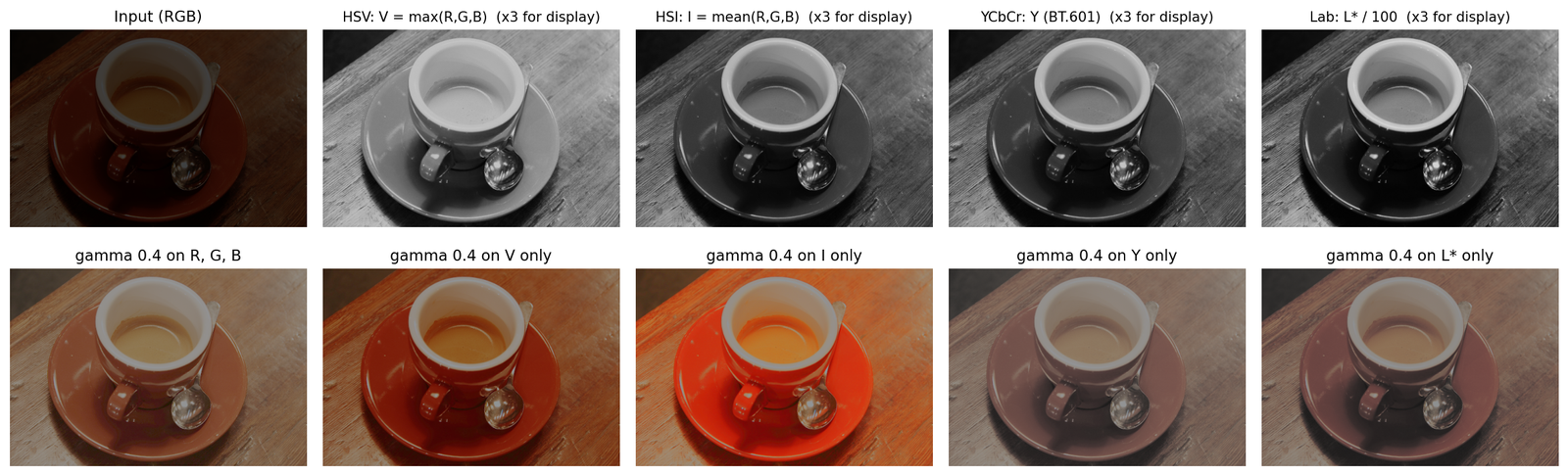
Two effects are visible. Scaling RGB by a common factor (HSV, HSI) preserves hue and keeps the ratio between channels, so HSV saturation is unchanged before clipping; their perceived colorfulness can still increase with brightness. Changing only or while keeping Cb/Cr or a*/b* fixed adds brightness without adding color, so the image looks washed out. This coupling of tone and color is exactly what later methods such as HVI-CIDNet [6] try to handle with a learned color space.
Histogram equalization and CLAHE
Plain version. Histogram equalization redistributes intensity values across the available range, expanding dark images’ concentrated values but potentially amplifying noise.
Precise version. For an image with levels, normalized histogram , HE uses the scaled cumulative distribution function as the mapping:
where is the number of pixels at level and the image size. The slope of is proportional to the histogram, so heavily populated gray levels get pulled apart. The derivation is in IP 03. For color images, the usual recipe is to convert to a space with a brightness channel, equalize that channel only, and convert back, for example RGB → Lab → equalize → RGB.
Global HE has two problems in low light: it over-stretches large flat regions (including their noise), and one mapping cannot serve both a dark corner and a bright lamp. Adaptive HE computes a mapping per tile, and CLAHE (contrast-limited AHE) clips each tile’s histogram at a limit before computing the CDF, which caps the slope of and therefore the noise gain, then interpolates between neighboring tiles to avoid seams [7], [8].
Optional: CLAHE: equalizing locally without amplifying noise (in the Supplementary notes). The clipping step and the tile blending written out as formulas, with a small experiment on noise gain.
Gamma correction
A power law with lifts shadows more than highlights; its slope is large near . It is cheap and monotonic but global: one for the whole picture, no denoising, and the same desaturation-or-oversaturation choice as above depending on where it is applied.
Code · Python · 10 lines
from skimage import color, exposure

gamma_out = dark ** 0.4                                     # power-law curve on every channel
lab = color.rgb2lab(dark)
L = lab[..., 0] / 100                                       # L* scaled to [0, 1]
he = lab.copy();    he[..., 0] = 100 * exposure.equalize_hist(L)
clahe = lab.copy(); clahe[..., 0] = 100 * exposure.equalize_adapthist(L, clip_limit=0.01)
he_out, clahe_out = color.lab2rgb(he), color.lab2rgb(clahe)
for name, im in [("gamma", gamma_out), ("HE", he_out), ("CLAHE", clahe_out)]:
    print(f"{name:6s} mean {im.mean():.3f}   std {im.std():.3f}")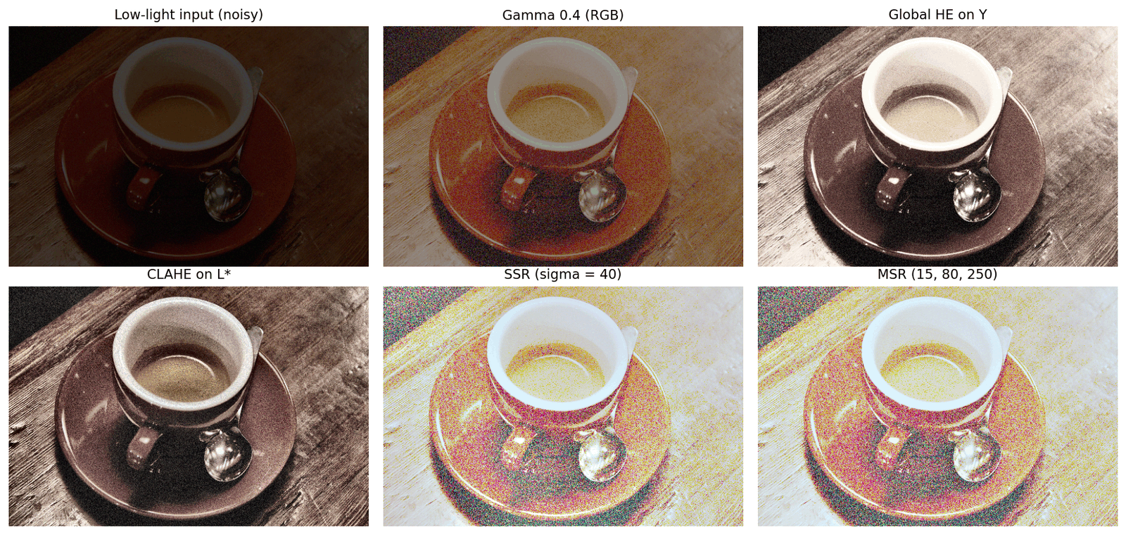
Retinex theory
Plain version. Retinex says that what the eye (or camera) receives is “the object’s own colors” multiplied by “the light falling on it”. If we can estimate the light, we can divide it out and see the object as it really is, then put back a better light.
Precise version. Land’s Retinex theory [9] models an observed image as
where is the pixel position, is the reflectance (a simplified surface-related component, assumed consistent across the paired lighting conditions), is the illumination (the light falling on the scene, which varies smoothly in space except at shadow boundaries), and is element-wise multiplication. Note the word: is illumination, not luminance. “Luminance” usually refers to a brightness channel of a color space, such as above.
Recovering two unknowns from one product is ill-posed, so every Retinex method adds a prior. The classic one is “illumination is smooth”.
Single-scale Retinex (SSR) [10] estimates with a Gaussian blur and works in the log domain, where the product becomes a sum:
for each color channel , with convolution and the surround scale. Small gives strong local contrast and halos at edges; large gives better tone but weaker detail. Multi-scale Retinex (MSR) [11] averages SSR outputs at several scales (typically three) with weights :
Because SSR and MSR work per channel, they tend to gray out the colors. MSRCR (MSR with color restoration) [11] multiplies the result by a color-restoration factor based on each channel’s share of ; other variants apply MSR to an intensity channel only and keep the input’s chromaticity.
Code · Python · 10 lines
from scipy import ndimage as ndi

def ssr(img, sigma=40.0, eps=1e-3):
    log_s = np.log(img + eps)
    log_l = np.log(ndi.gaussian_filter(img, sigma=(sigma, sigma, 0)) + eps)  # L ~ Gaussian blur
    r = log_s - log_l                                       # log R = log S - log L
    lo, hi = np.percentile(r, [1, 99])                      # robust stretch for display
    return np.clip((r - lo) / (hi - lo), 0, 1)

msr = np.mean([ssr(dark, s) for s in (15, 80, 250)], axis=0)   # MSR, equal weights (simplified)
For enhancement we usually do not want alone, which looks flat and unnatural. We want to brighten and recombine: with, for example, and . This “decompose, adjust , recombine” pattern is the template for most Retinex-based deep networks.

LIME: Retinex as optimization
LIME [4] estimates only the illumination. It initializes it with the bright channel, , then refines it by solving a structure-aware smoothing problem: keep close to , but make it smooth except where the image has strong structure. The enhanced image is (equivalently when ), and because dividing amplifies noise, LIME optionally denoises afterward. LIME’s images (often called the LIME set) became a standard test set, and the method is a good example of the classical recipe: a physical model, a hand-designed prior, and an optimization.
Another model: dehazing an inverted image
The Retinex model is not the only image-formation model. Dehazing uses the atmospheric scattering model, written out in DLCV 09: a hazy observation is the haze-free scene radiance attenuated by a transmission , plus a global atmospheric light . This model cannot be applied to a dark image directly, because a dark image does not look like a hazy one.
Dong et al. observed that an inverted low-light image, , does look hazy: dark regions become bright and low-contrast, like fog. They therefore invert the image, run a dehazing algorithm (in the spirit of the dark channel prior [3]), and invert the result back [12]. With the hazy image and the haze-free result, the inversions are
From the “what is reliable” angle, dehazing assumes the dark channel marks haze-free content; in a low-light image the dark channel is mostly damaged pixels, so attention shifts to the bright channel, the region least affected by the darkness. The LIME paper [4] analyzes this inversion approach and shows that it can be rewritten in Retinex form, so the two models make essentially the same assumption, with Retinex being the simpler statement.
Statistical approaches
Many classical methods add statistics or priors on top of these models: naturalness constraints that keep the lightness order of a scene (NPE [13]), layered or two-dimensional histogram models (the method behind the DICM set [14]), and fusion of several synthetic exposures. They are hand-crafted, need no training data, and generalize in a predictable way; their weak point is noise, which they usually ignore or hand to a separate denoiser.
Deep-learning LLIE
Two axes: learning signal and design lineage
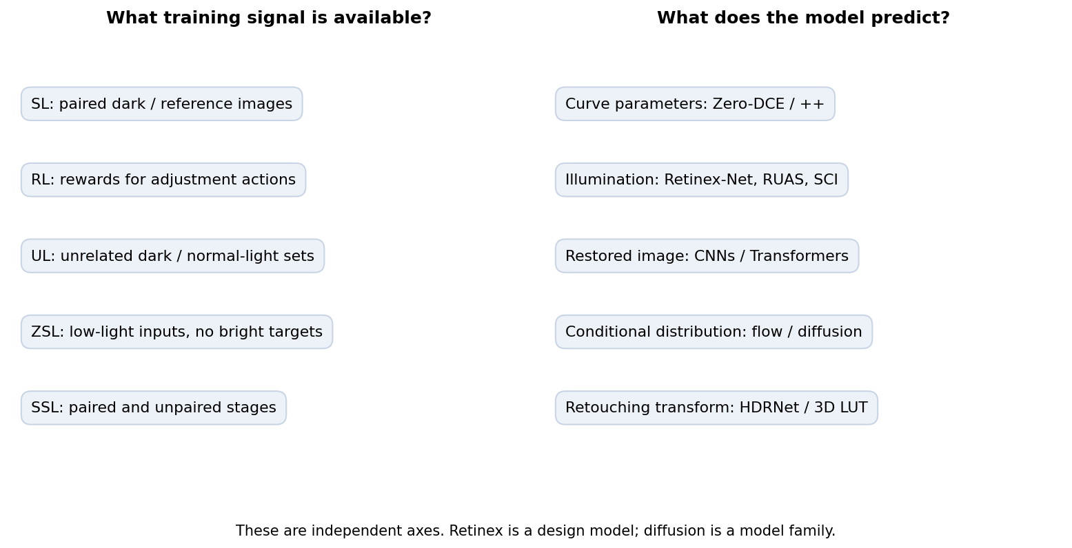
A model’s architecture and its supervision are separate choices. Following Li et al.’s survey [15], supervised learning (SL) uses paired dark/reference images; reinforcement learning (RL) uses rewards for a sequence of adjustments; unsupervised learning (UL) uses unpaired dark and normal-light sets; zero-shot learning (ZSL) in that survey uses low-light data alone, sometimes optimizing on the test image; and semi-supervised learning (SSL) combines paired and unpaired stages. Here SSL means semi-supervised, not self-supervised. Other papers use “unsupervised,” “zero-reference” and “self-supervised” differently, so inspect their actual data requirements.
The design axis asks what is predicted: curve parameters, illumination, image residuals, a generative denoising trajectory, or a compact retouching transform. Retinex can appear under several learning strategies; diffusion is a model family, not a supervision category.
| Method | Design and learning signal | Quality mechanism | Published cost and scope |
|---|---|---|---|
| Retinex-Net [16] | Decomposition and illumination adjustment; paired images, no intrinsic-image labels | Reflectance consistency and structure-aware smoothness | Several learned stages plus optional reflectance denoising; measure the complete pipeline |
| EnlightenGAN [17] | Image generator; unrelated dark/normal-light sets | Global/local adversarial and self-feature constraints | Discriminators are training components; deploy the generator |
| Zero-DCE [18] | Spatially varying curves; no reference images | Exposure, color, local-contrast and parameter-smoothness priors | 79,416 parameters; 84.99 G FLOPs at 1200 × 900 in [19], Table 4 |
| Zero-DCE++ [19] | Shared curves estimated on a thumbnail; no references | Same family of priors with less flexible curve prediction | 10,561 parameters; 0.115 G FLOPs at 1200 × 900 in [19], Table 4 |
| RUAS [20] | Searched unrolled illumination/denoising modules; reference-free losses | Retinex structure plus a separate noise-removal stage | Illumination-only 0.001 M parameters versus illumination-plus-denoising 0.003 M, as rounded in its Table 2 |
| SCI [21] | Illumination estimation; unsupervised training cascade | Self-calibration during training; one basic block at inference | 0.0003 M parameters, rounded in its Table 4; calibration module is not deployed |
| Retinexformer [22] | Illumination-guided Transformer; paired images | Noise/artifact restoration guided by illumination features | 1.61 M parameters, 15.57 G FLOPs at 256 × 256, Table 4 |
| LLFlow and diffusion methods [23], [24], [25], [26], [27] | Conditional generative restoration; supervision varies | Learned conditional distribution or image prior | Count all network evaluations, image encoding and decoding; not comparable from parameter count alone |
| HDRNet [28] | Local affine bilateral grid; paired photographic edits | Local/global context chooses a spatially varying transform | Thumbnail prediction plus full-resolution guide, slicing and application |
| Image-adaptive 3D LUT [29] | Basis color tables; paired or unpaired retouching data | Image-dependent global color transform | 1.66 ms at 3840 × 2160 on one Titan RTX, its Table 7 |
These rows use different resolutions, counting conventions and timing hardware. They explain design choices, not a common speed ranking. The LUT timing is a photographic-retouching result; it does not establish denoising quality on a dark phone capture. For a first comparison, run a fixed gamma baseline, inspect the photon experiment, then try the curve toy. Read detailed architectures after the image and evaluation problems are clear.
Supervised methods (paired data)
Training on pairs of low-light and normal-light images follows the general recipe of DLCV 09: fit with a reconstruction loss, typically plus perceptual or structural terms (see DLCV 09 for these losses). Paired data is expensive (two exposures of a static scene, or synthesis), and the network learns the specific brightness and color style of the reference images, which matters for evaluation later.
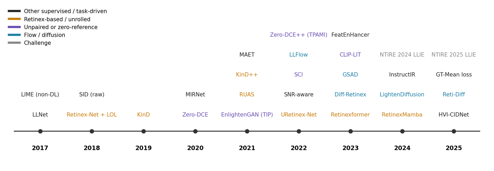
Representative examples: LLNet [30] (2017), one of the first deep LLIE models, learned brightening and denoising jointly with a denoising autoencoder; Tao et al. [31] (2017) denoised with a CNN and then enhanced contrast with a bright-channel model; MIRNet [32] (2020) is a general multi-resolution restoration backbone; SNR-aware [33] (2022) estimates a per-pixel signal-to-noise map and uses long-range attention where the local neighborhood is too noisy to trust; and HVI-CIDNet [6] (2025) learns a color space that decouples color from intensity, attacking the problem of Figure 2.
Optional: More deep LLIE methods (in the Supplementary notes). How each of these five networks is built.
Efficient end-to-end designs
A direct network can learn restoration as well as tone adjustment, at a cost that grows with its spatial feature maps. IAT [34] combines local multiply/add maps with global color-matrix and gamma prediction. Thin convolutions, depthwise filtering and a small global branch reduce computation, while a compact network can still fail on noise patterns absent from training.
Structural re-parameterization trains several linear branches and merges them into one convolution for inference [35]. It changes deployment structure, whereas weight sharing changes stored parameters. Neither guarantees faster execution on every device. Measure the exported model, including its full-resolution operations.
Optional: Efficient network building blocks and Structural re-parameterization step by step (in the Supplementary notes). Architectural details and an executed fusion-equivalence check.
Retinex-based networks
Retinex-Net [16] (2018) changed the goal from “estimate ” to “both the input and the output have their own and ”. The pipeline is: decompose the low and normal images, enhance to , recombine with . It also introduced the LOL dataset (below). Its paired-image training enforces reconstruction, reflectance consistency across exposures and structure-aware illumination smoothness. There are no measured intrinsic reflectance/illumination targets: the components are useful learned representations, not uniquely identified physical quantities. A separate illumination-adjustment network changes brightness, and reflectance denoising addresses amplified noise.
Optional: Retinex-Net (in the Paper guides). The complete cross-reconstruction objective, architecture and qualitative ablations.
The pattern spread quickly. KinD [36] (2019) and KinD++ [37] (2021) add a reflectance-restoration step, because the dark image’s reflectance is noisy and color-shifted; Retinexformer [22] (2023) adds perturbation terms for noise and artifacts to the Retinex model, trains in one stage, uses the illumination estimate to guide self-attention, and became a common baseline; RetinexMamba [38] (2024 preprint) swaps attention for Mamba state-space blocks. “Retinex decomposition plus a new backbone” has been a stable design pattern for years. A less common route builds lightweight networks on the atmospheric scattering model instead (CPGA-Net [39], CPGA-Net+ [40]).
Optional: More deep LLIE methods (in the Supplementary notes). Retinexformer’s perturbed Retinex model and the prior-guided CPGA-Net line in more detail.
Quality and cost within the same lineage
Predicting a smooth transform on a thumbnail can preserve full-resolution detail because the original pixels are still available when the transform is applied. It cannot recover information that clipping or noise removed. If the desired operation is denoising or deblurring, a pointwise transform alone is insufficient; a network that predicts that transform from a neighborhood can still use context, so “curve-based” does not imply that the complete system has no spatial reasoning.
For illumination models, division by a small illumination estimate amplifies both detail and noise. A separate reflectance-restoration module costs more but addresses a different problem from tone adjustment. The experiment below contrasts resizing a smooth illumination map with resizing the already enhanced image. Its reference is the same toy operator run at full resolution, not a real normal-light ground truth.
It estimates the illumination in a simple classical way: the bright channel (the per-pixel maximum of R, G and B), which LIME [4] uses as its initial estimate, smoothed here with a plain Gaussian instead of LIME’s structure-aware refinement. It does so once at full resolution and once on an 8× smaller copy (1/64 of the pixels), and compares two ways of producing the full-resolution result.
Code · Python · 26 lines
import numpy as np
from scipy.ndimage import gaussian_filter
from skimage import data, img_as_float
from skimage.metrics import peak_signal_noise_ratio as psnr
from skimage.transform import resize

dark = (0.15 * img_as_float(data.coffee()) ** 2.2) ** (1 / 2.2)   # 400 x 600, 15% of the light

def illumination(x, sigma):
    """A simple illumination estimate: the bright channel (max of R, G, B), smoothed."""
    return np.clip(gaussian_filter(x.max(axis=-1), sigma), 0.02, 1)

def relight(x, L, gamma=0.4):
    """Retinex relighting: O = R * L**gamma = I * L**(gamma - 1)."""
    return np.clip(x * L[..., None] ** (gamma - 1), 0, 1)

reference = relight(dark, illumination(dark, sigma=15))           # estimate L at full resolution
small = resize(dark, (50, 75), anti_aliasing=True)                # 8x smaller in each direction
L_small = illumination(small, sigma=15 / 8)                       # estimate L on 1/64 of the pixels
results = {
    "L at 1/8 size, resized up": relight(dark, resize(L_small, dark.shape[:2], order=1)),
    "relight at 1/8 size, resize output": resize(relight(small, L_small), dark.shape, order=1),
}
print(f"mean brightness {dark.mean():.2f} -> {reference.mean():.2f}")
for name, out in results.items():
    print(f"{name:36s} PSNR vs full-resolution estimate {psnr(reference, out, data_range=1):5.2f} dB")
Output
mean brightness 0.16 -> 0.35
L at 1/8 size, resized up            PSNR vs full-resolution estimate 54.57 dB
relight at 1/8 size, resize output   PSNR vs full-resolution estimate 22.87 dB
Resizing the map is almost indistinguishable from the full-resolution estimate (above 54 dB on our toy), while resizing the output loses about 31.7 dB, because the image’s detail is gone. It works because this light map is very smooth; one with sharp shadow boundaries suffers more, which is why some methods upsample it with an edge-aware step.
Retinex-inspired unrolling
Unrolling (or unfolding) takes an iterative optimization algorithm for the Retinex problem and turns each iteration into a network stage with learnable parameters. The architecture inherits the algorithm’s structure and interpretability, and training replaces hand-tuned priors.
- RUAS [20] (2021) unrolls optimization models for illumination estimation and noise removal, searches the architecture of the prior modules, and is trained with a cooperative reference-free strategy, so it also belongs in the unsupervised column. It is very small and fast.
- URetinex-Net [41] (2022) unfolds a Retinex decomposition optimization into a network with learned modules for initialization, the unfolded updates of and , and illumination adjustment.
Unpaired training: EnlightenGAN
EnlightenGAN [17] (2021) uses a generative adversarial network (GAN) so that it needs only a set of dark images and an unrelated set of well-lit images. A U-Net generator, guided by a self-regularized attention map derived from the input’s illumination, produces the enhanced image. A global discriminator judges the whole image and a local discriminator judges random patches, so the output looks like a well-lit photo both overall and in detail. A self-feature-preserving loss compares VGG features of input and output, keeping content in place since there is no ground truth to do so.
Zero-reference methods and curve estimation
Plain version. Zero-DCE does not output a new image. It outputs a brightening curve per pixel, applies it, and is trained with losses that judge the result without any reference photo: “is it well exposed, is the color balanced, is the curve smooth, is local contrast kept?”
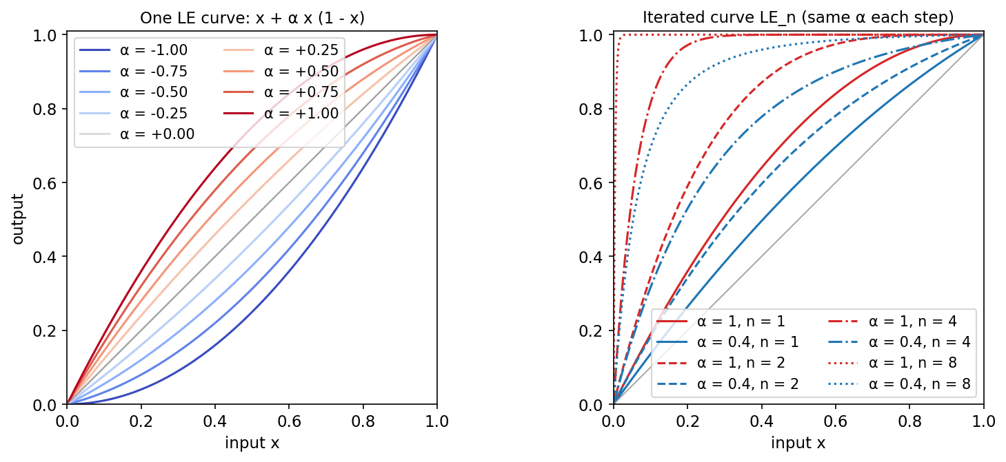
The LE curve. Zero-DCE [18] (2020) defines a quadratic light-enhancement curve
where is a pixel value. The curve has three useful properties: and , so the range is preserved and no clipping is needed; it is monotonic for , because , so a fixed curve preserves order; different spatial parameter maps need not preserve ordering between pixels; and it is differentiable, so it can be trained by backpropagation. One quadratic is not flexible enough, so it is applied iteratively:
with the input, , and a per-pixel, per-channel parameter map instead of a single . A seven-layer CNN (DCE-Net, 32 channels per layer, about 79k parameters, no downsampling) predicts maps with a tanh output. Each pixel thus gets its own high-order curve, which is how local adjustment arises from a global-looking formula.
Code · Python · 10 lines
def le_iterate(x, alphas):
    """Zero-DCE curve: LE_n = LE_{n-1} + a_n * LE_{n-1} * (1 - LE_{n-1})."""
    y = x.copy()
    for a in alphas:              # a can be a scalar or a per-pixel map
        y = y + a * y * (1 - y)
    return y

x = np.array([0.0, 0.02, 0.1, 0.3, 0.6, 1.0])
print(le_iterate(x, [1.0] * 8).round(3))   # [0. 0.994 1. 1. 1. 1.]
print(le_iterate(x, [0.4] * 8).round(3))   # [0. 0.245 0.695 0.93 0.985 1.]
The first line shows the danger: for small , each step multiplies by about , so eight steps with give a gain near . Whatever noise sits in the shadows is amplified by the same factor.
Non-reference losses. Training uses four complementary priors: retain local contrast, move patch-mean brightness toward a selected exposure target, discourage global RGB color imbalance, and smooth the parameter maps. None is a measured normal-light target. Gray-world balance can damage a colorful scene; the exposure target is a preference; smooth curves can still amplify noise. The original paper uses exposure target 0.6 and eight iterations [18].
Optional: Zero-DCE and Zero-DCE++ (in the Paper guides). Full architecture, objectives, quantitative ablations and the distinction between a fixed monotonic curve and spatially varying parameters.
Follow-ups refined the idea:
- Zero-DCE++ [19] (2022) uses depthwise separable convolutions, predicts only 3 curve maps and reuses them across all iterations, and estimates them on a downsampled input before resizing them back. This cuts the model to about 10k parameters and makes it fast enough to run at interactive rates even on a CPU.
- SCI [21] (2022) learns illumination with a cascade of weight-sharing stages and a self-calibrated module that makes the stages’ outputs converge during training, so that at test time a single basic block suffices. It is trained with unsupervised losses.
- CLIP-LIT [42] (2023) targets backlit images. It uses the vision-language model CLIP and learns a pair of text prompts, one for backlit and one for well-lit images, then refines the prompts and the enhancement network iteratively, so the CLIP similarity to the “well-lit” prompt acts as the training signal.
A zero-reference toy in PyTorch
To see these losses at work, the code below trains a tiny Zero-DCE-style network for about half a minute on CPU. It trains on random crops of four skimage images, each darkened by a random factor in linear light, and is tested on the coffee image, which it never sees during training. No ground truth is used. (The loss weights differ from the paper’s because the terms are normalized differently: squared rather than absolute exposure error and mean rather than summed gradients.)
Code · Python · 58 lines
import numpy as np
import torch
torch.set_num_threads(1)
import torch.nn as nn
import torch.nn.functional as F
from skimage import data, img_as_float
from skimage.transform import resize

torch.manual_seed(0); rng = np.random.default_rng(0)
darken = lambda x, k: (k * x ** 2.2) ** (1 / 2.2)          # less light, in linear units
train = [resize(img_as_float(f()), (256, 256), anti_aliasing=True)
         for f in (data.astronaut, data.chelsea, data.rocket, data.immunohistochemistry)]

def batch(n=4, size=64):                                  # random crops, random darkness
    xs = []
    for _ in range(n):
        img = train[rng.integers(len(train))]
        i, j = rng.integers(0, 256 - size, 2)
        xs.append(darken(img[i:i + size, j:j + size], rng.uniform(0.02, 0.3)))
    return torch.tensor(np.stack(xs), dtype=torch.float32).permute(0, 3, 1, 2)

class TinyDCE(nn.Module):
    def __init__(self, n_iter=8, w=16):
        super().__init__()
        self.n_iter = n_iter
        self.body = nn.Sequential(
            nn.Conv2d(3, w, 3, padding=1), nn.ReLU(), nn.Conv2d(w, w, 3, padding=1), nn.ReLU(),
            nn.Conv2d(w, w, 3, padding=1), nn.ReLU(), nn.Conv2d(w, 3 * n_iter, 3, padding=1), nn.Tanh())
    def forward(self, x):
        alphas = self.body(x).chunk(self.n_iter, dim=1)    # 8 maps of shape B x 3 x H x W
        y = x
        for a in alphas:
            y = y + a * y * (1 - y)                         # the LE curve
        return y, torch.cat(alphas, 1)

def L_exp(y, E=0.6, p=16):   # mean brightness of 16x16 patches should be near E
    return (F.avg_pool2d(y.mean(1, keepdim=True), p) - E).pow(2).mean()
def L_col(y):                # gray-world: channel means should agree
    r, g, b = y.mean((2, 3)).unbind(1)
    return ((r - g) ** 2 + (r - b) ** 2 + (g - b) ** 2).mean()
def L_tv(a):                 # curve parameters should vary smoothly in space
    return (a[..., 1:, :] - a[..., :-1, :]).pow(2).mean() + (a[..., :, 1:] - a[..., :, :-1]).pow(2).mean()
def L_spa(y, x, p=4):        # keep the contrast between neighbouring 4x4 regions
    Y, X = (F.avg_pool2d(t.mean(1, keepdim=True), p) for t in (y, x))
    return sum(((torch.diff(Y, dim=d) - torch.diff(X, dim=d)) ** 2).mean() for d in (2, 3))

net = TinyDCE()
opt = torch.optim.Adam(net.parameters(), lr=1e-3)
for step in range(600):                                   # small CPU training experiment
    x = batch()
    y, a = net(x)
    loss = L_spa(y, x) + 10 * L_exp(y) + 5 * L_col(y) + 200 * L_tv(a)
    opt.zero_grad(); loss.backward(); opt.step()

test = darken(img_as_float(data.coffee()), 0.05)          # an image never used in training
with torch.no_grad():
    out, _ = net(torch.tensor(test, dtype=torch.float32).permute(2, 0, 1)[None])
print(f"mean brightness: {test.mean():.3f} -> {out.mean():.3f}")   # about 0.10 -> 0.50
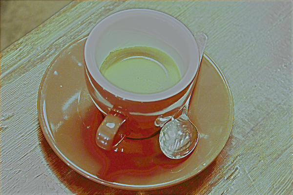
Drag the slider to compare the dark input and the toy’s output:

 Dark inputZero-reference toy
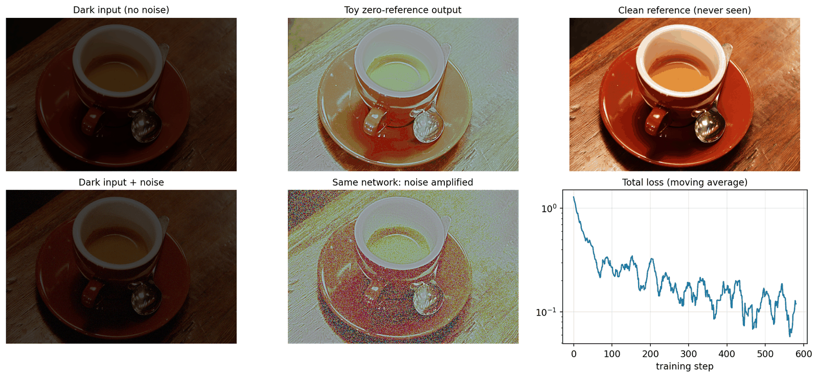
The toy shows the strengths and the limits of the zero-reference idea in one picture. Without a single reference image, the network learns a sensible brightening that transfers to an unseen photo. But each loss is a prior, and priors can be wrong: gray-world fails for scenes that really are red or brown, a fixed exposure target flattens deliberately dark regions, and nothing in the losses asks for denoising. Real zero-reference methods are trained on many more images, and some add explicit noise handling, but these failure modes are visible in published results too.
Normalizing flows and diffusion models
LLFlow [23] (2022) observes that one dark image has many acceptable bright versions, and a pixel-wise loss averages them into a blurry compromise. It learns a conditional normalizing flow: an invertible network that maps normal-light images to a Gaussian distribution, conditioned on features of the dark input. Those features are guided by priors that echo the classical methods: a histogram-equalized version of the input, a color map (close to the Retinex reflectance) and a noise map.
From 2023, diffusion models entered LLIE. They generate the output by iteratively denoising random noise, conditioned on the dark image, and so can synthesize plausible detail that regression networks blur out. Diff-Retinex [24] generates the Retinex reflectance and illumination with diffusion, LightenDiffusion [26] decomposes in a latent space and trains on unpaired data, Reti-Diff [27] uses latent diffusion only to produce compact priors for a restoration transformer, and GSAD [25] regularizes the diffusion trajectory with the image structure. The trade-off is cost and fidelity: many denoising steps make inference slow, and generated details may look right without being true.
Optional: More deep LLIE methods (in the Supplementary notes). What each diffusion model adds, and a survey taxonomy of the sub-field.
Real-time photographic transforms
HDRNet [28] and image-adaptive 3D LUTs [29] originated in photographic retouching. They predict a compact transform from a thumbnail and apply it to the original pixels. This can retain input detail at high resolution, but a fast tone/color edit is not a complete sensor-noise restoration pipeline.
A bilateral grid stores spatially varying affine transforms. A full-resolution guide supplies the third coordinate, allowing pixels near an edge to select different transforms. After interpolating eight nearby nodes, apply the resulting 3 × 4 matrix to RGB plus a constant bias. HDRNet learns the guide and coefficients from paired edits; the optional experiment instead fits coefficients by weighted least squares, so it is a conceptual toy rather than the original learned model.
A 3D LUT is indexed by RGB rather than spatial position. It stores a transform on an color lattice, with three output values per node. Trilinear interpolation combines eight enclosing colors. An image-adaptive model predicts coefficients for basis tables and forms
Here is the number of bases and is the image’s combined table. Fusing the tables once and interpolating once per pixel equals interpolating every basis and combining the outputs, because interpolation is linear in table values. A global LUT maps identical RGB values identically everywhere in one image; it cannot independently brighten one of two same-colored regions.
The default adaptive LUT uses three 33-node bases [29]. Table size grows as values, so finer lattices trade memory for accuracy near steep dark-region curves. Learned nonuniform nodes and spatial/context extensions change that trade-off [43], [44], [45], [46], [47]. The full method and measured results are in the paper introductions.
Optional: Bilateral grids and color-table mathematics, A bilateral-grid experiment and Implementing and checking trilinear LUTs (in the Supplementary notes). Definitions, original toy code and interpolation checks.
Raw-domain low light
Everything above works on processed sRGB images, where the camera’s pipeline (demosaicking, white balance, denoising, tone curve, compression) has already discarded information. Learning to See in the Dark [48] (2018) instead feeds raw sensor data to a U-Net that replaces the whole pipeline. Its SID dataset has 5,094 short-exposure raw images paired with 424 distinct long-exposure references, from a Sony α7S II (Bayer sensor) and a Fujifilm X-T2 (X-Trans sensor), with exposure ratios of ×100, ×250 and ×300. Raw data keeps the linear relation between photons and values and has more bits, so extreme low light that is hopeless in sRGB becomes recoverable. The cost is that the model is tied to one sensor.
All-in-one restoration
Low-light enhancement is also one task inside all-in-one restoration models, for example InstructIR [49] (2024), which restores an image according to a natural-language instruction such as “make this photo brighter”. The all-in-one family as a whole is described in DLCV 09.
Low light for downstream tasks
If the goal is detection rather than pretty pictures, the usual baseline is “enhance, then detect” (see DLCV 03 · Object Detection). But enhancement tuned for people is not necessarily what a detector needs. MAET [50] (2021) models the low-light degradation physically and trains the detector to also predict the degradation parameters, so that features become aware of it. FeatEnHancer [51] (2023) enhances hierarchical features inside the network, trained directly with the downstream loss, instead of enhancing pixels.
Measuring efficiency honestly
Plain version. Efficiency claims are easy to make and hard to compare. A fair comparison of lightweight designs says exactly what was counted, at which resolution, on which hardware, and includes every step from input frame to output frame.
Dehghani et al. show that parameters, FLOPs, throughput and latency can disagree, and that reporting only one of them gives a misleading picture [52]. For enhancement:
- Count at the deployment resolution, and also report MACs per megapixel so that readers can rescale. A FLOP count at 256 × 256 says nothing about 4K for a full-resolution network, and the opposite is true for thumbnail-based designs.
- Include the full-resolution step. Slicing, LUT interpolation, curve iteration, guided-filter upsampling and resizing are often custom operators that automatic FLOP counters skip. They are the part of a predict-then-apply design that grows with resolution.
- Say what a “parameter” includes. A 33-node 3D LUT is about 108K values, more than the whole of Zero-DCE++ at about 10K parameters [19] or IAT at about 90K [34].
- Time the whole path on the target device: fixed device, runtime, numeric precision, batch size 1, resolution and thread count, warm-up, percentiles, GPU synchronization, and color conversion and memory transfers included (the protocol of ML 11). Challenges that time on real phones make this concrete: the Mobile AI 2022 learned-ISP challenge, for example, measured runtime on a Snapdragon 8 Gen 1 GPU with TensorFlow Lite [53]. A GPU number from a paper (such as the Titan RTX or V100 timings above) tells you about relative speed on that GPU, not about your phone.
- Judge quality at full resolution, with the metrics of DLCV 09 and the low-light specifics of DLCV 09C, because halos and banding from coarse grids or tables may vanish when the output is downsampled for scoring.
Optional: Counting resolution, arithmetic and memory (in the Supplementary notes). A numerical comparison of three toy architectures. For pruning, quantization and distillation, continue to DLCV 01C.
Failure modes
| Symptom | Why it happens | What to check |
|---|---|---|
| Bright grain and false texture | Shadow gain amplifies sensor noise | Flat-region crops and a noise-aware restoration stage |
| Posterized gradients | A few quantized dark levels are spread far apart | Input bit depth and near-black ramps |
| Halos | A coarse illumination map or bilateral cell spans a sharp boundary | Full-resolution edges, grid size and guide behavior |
| Unnatural color | Gray-world priors, clipping or sparsely trained LUT regions | Skin, neon lights and strongly colored scenes |
| Flickering video | Per-frame parameters change abruptly | Temporal parameter traces and moving scenes |
| Good scores, poor recognition | The metric objective differs from the downstream task | A fixed, disclosed task protocol as well as visual evaluation |
A global LUT cannot map identical colors differently by position, and a fixed pointwise transform cannot average independent spatial noise. Spatially predicted curve parameters can use neighboring evidence, so diagnose the complete architecture rather than assuming every curve model has the same limits.
Optional: Banding, halos and temporal stability (in the Supplementary notes). A tested bit-depth example and detailed failure analysis.
Evaluation
Plain version. The general evaluation toolkit (full-reference and no-reference metrics, learned and vision-language assessors, user studies, and the pitfalls and reporting practice that go with them) is explained once, in DLCV 09. This section does not repeat it. It covers what is different for dark images: why no-reference scores matter so much here, how the common ones mislead on exposure and color, measures made for enhancement, the GT-mean pitfall, and task-driven evaluation.
Full-reference metrics
On paired sets, LLIE papers report PSNR, SSIM [54] and LPIPS [55] exactly as defined in DLCV 09. The one low-light-specific caution is brightness: a small global exposure difference from the reference costs a lot of PSNR, which is the subject of the GT-mean pitfall below.
No-reference metrics: why low light depends on them
Plain version. A no-reference (NR) metric looks at one image and guesses how good it is, with no “correct answer” to compare against. Low-light papers need these metrics because their most realistic test photos have no correct answer, and because even when one exists, it is only one of many acceptable brightness levels.
Precise version. Two facts push LLIE toward NR evaluation:
- Real test sets are unpaired. LIME [4], MEF [56], NPE [13], DICM [14] and VV [57] are small sets of real, often non-uniformly lit photos with no ground truth. Paired sets such as LOL [16] exist, but they were captured under controlled conditions (a static scene, two exposures), and a model can do well on them without generalizing (the generalization gap reported in [15]). Results on the unpaired sets are therefore shown in almost every LLIE paper, and only NR metrics and human judgments can score them.
- The “correct” brightness is ambiguous. Even with a reference, the normal-light image is one photographer’s choice of exposure and color. An output that is a little brighter or warmer can look as good, yet lose several dB of PSNR (this is the reason for the GT-mean protocol below). An NR metric at least does not punish a different but valid exposure.
The price is that an NR metric is a model of human preference, and every model has blind spots. The general theory of no-reference image quality assessment (IQA), including how NIQE, BRISQUE, MUSIQ and CLIP-IQA are built and how NR metrics are validated against human opinion, is covered in DLCV 09. The subsections below do not repeat it; they focus on how each family behaves on enhanced low-light images.
Classical natural-scene-statistics metrics: NIQE, BRISQUE and PI
NIQE [58], BRISQUE [59] and the Perceptual Index (PI) [60], [61] are natural-scene-statistics (NSS) metrics: they measure how far the statistics of an image (its MSCN coefficients) are from those of clean photos, and lower is better for all three. The MSCN coefficients and the BRISQUE and NIQE constructions are given in DLCV 09, together with a runnable snippet showing how blur, noise and over-sharpening move the features; the definition of PI is in the DLCV 09 notes. Low-light papers use these metrics heavily; Zero-DCE [18], for example, reports PI on the unpaired sets alongside a user study.
What they reward, and how they mislead on exposure. All three were designed for structural distortions (blur, noise, compression, ringing), not for exposure or color:
- MSCN normalization divides out local mean and contrast by construction, so a global brightness change barely moves the features. An under-enhanced image and a well-exposed one can get similar scores.
- Grayscale features ignore color casts and saturation, the very errors of Figure 2.
- Noise and over-sharpening add high-frequency energy, which can make a smooth, noise-amplified output look “more natural” to these statistics than a clean but slightly soft one. HE and CLAHE outputs, with strong local contrast, are a typical case.
- The pristine corpus and training distortions contain few dark, night or backlit scenes, so “natural” means “daylight-like”.
No-reference measures need complementary checks
A low-light metric can reward the wrong change. Lightness order error (LOE) measures how often relative brightness ordering changes [13]; it does not check whether the result is bright enough. Colorfulness [62] measures opponent-color variation and can rise when chroma noise is amplified. Noise estimates depend on separating texture from noise [63]. Learned quality models discussed in the optional note inherit their training domains, which may contain few severely dark images.
Use several metric families, show full-resolution crops, and specify the preprocessing and implementation. For human comparisons, randomize order and state the viewing conditions and question; photographic preference and task usefulness are distinct outcomes. A source image is available at test time, but its brightness is not the desired brightness target.
Optional: Understanding no-reference low-light metrics (in the Supplementary notes). Precise LOE/colorfulness/noise definitions, tested counterexamples, learned assessors and a reporting protocol.
The GT-mean pitfall
Plain version. On paired benchmarks, a small difference in overall brightness changes PSNR a lot. Some papers rescale each output so its average brightness matches the ground truth before scoring. That is information you never have in practice.
Precise version. “GT-mean” evaluation scales the output by and computes the metric on , where is the image mean. Because LLIE is ambiguous about the “right” brightness, this can raise PSNR substantially. The Retinexformer authors provide this mode in their code for comparability with methods such as LLFlow and KinD and recent diffusion models, while explicitly saying they do not recommend it, because it uses the ground truth to correct the output [22]. Liao et al. [64] (2025) study the brightness mismatch between outputs and references and propose a GT-mean loss for training, reporting both standard and GT-mean metrics. When reading tables: check which setting is used, never mix the two, and prefer methods that are good under the standard protocol.
Task-driven evaluation
Since LLIE is often a preprocessing step, another test is to run a detector or segmenter on the enhanced images (on ExDark [65], for example) and report its accuracy. Liu and Fan’s 2025 review [66] finds a disconnect: supervised methods often produce images with high perceptual quality but only modest gains for vision tasks, while zero-shot methods, despite lower image-quality scores, give more consistent gains across tasks. The benchmark of Liu et al. [67] also evaluates face detection in low light. A complete evaluation reports fidelity, no-reference quality, task performance, and runtime.
Benchmark datasets
Plain version. Datasets differ in whether they have pairs, whether the darkness is real or synthetic, whether they are raw or sRGB, and whether they carry labels for detection.
| Dataset | Type | Content and what it is for |
|---|---|---|
| LOL (v1) [16] | Paired, real, sRGB | 500 low/normal pairs captured by changing exposure (485 train / 15 test), 400×600. The most common LLIE benchmark; small test set. |
| LOL-v2 [68] | Paired, real + synthetic subsets | A larger Real subset of captured pairs and a Synthetic subset of synthesized pairs. Report the two subsets separately. |
| LSRW [69] | Paired, real | 5,650 pairs from a Nikon D7500 (3,170) and a Huawei P40 Pro (2,480); 5,600 train, 50 test. Tests generalization across devices. |
| SDSD [70] | Paired video | Dynamic indoor and outdoor scenes captured twice with a mechatronic system for alignment; often split into frames for image tests. |
| SID [48] | Paired, raw | 5,094 short-exposure raw images with 424 long-exposure references (Sony and Fuji). Extreme low light, raw-to-sRGB. |
| MIT-Adobe FiveK [71] | Paired, retouching | 5,000 raw photos, each retouched by five experts. Used for tone and color enhancement (photo retouching). |
| SICE [72] | Multi-exposure sequences | Under- to over-exposed captures of each scene with a reference; used to train exposure correction (e.g. Zero-DCE). |
| VE-LOL [67] | Paired + detection | VE-LOL-L for enhancement and VE-LOL-H with face annotations for high-level evaluation. |
| ExDark [65] | Unpaired, labeled | 7,363 low-light images, 12 object classes, 10 lighting conditions. Task-driven evaluation (detection). |
| LIME [4], MEF [56], NPE [13], DICM [14], VV [57] | Unpaired test sets | Small collections of real low-light or non-uniformly lit photos for visual comparison and no-reference metrics. |
Challenges: NTIRE 2024 and 2025
The NTIRE workshop at CVPR (see DLCV 09 for the series in general) ran LLIE challenges in consecutive years. The NTIRE 2024 challenge [73] covered ultra-high-resolution (4K and beyond), non-uniform illumination, backlighting, extreme darkness and night scenes; it had 428 registered participants and 22 teams with valid submissions. The NTIRE 2025 challenge [74] had 762 registered participants and 28 teams with valid entries. The reports summarize the winning designs and are a good snapshot of what works under a fixed, fair protocol.
Modern view
Li et al. [15] provide the learning-strategy taxonomy used above and compare generalization, cost and image quality under a common protocol. Their review includes real-phone image/video data and warns that a result on a paired benchmark need not transfer to a noisy phone capture. Zheng et al. [75] add mixed-exposure and video perspectives; VE-LOL [67] and the later task-oriented study [66] distinguish appearance from downstream utility. The diffusion review [76] organizes generative enhancement into six families, which differ in conditioning, representation and inference procedure. Read each survey as a dated map, then verify a recent method through its primary paper.
Efficient enhancement in 2026. The NTIRE efficient low-light challenge [77] uses a model-size constraint and rank aggregation over several quality metrics. A small file is not a measured phone latency. Its report illustrates compact encoder–decoders, color/illumination priors and re-parameterization under that particular protocol. HDRNet and LUT models instead originated in photographic retouching; they need separate low-light validation.
State of the art (2023–2026). Three directions dominate. First, Retinex-guided backbones: transformers (Retinexformer [22]) and state-space models (RetinexMamba [38]) that keep a light-versus-reflectance structure. Second, generative models: diffusion (Diff-Retinex [24], GSAD [25], LightenDiffusion [26], Reti-Diff [27]) and flows (LLFlow [23]). Third, better representations and protocols: learned color spaces (HVI-CIDNet [6]), brightness-mismatch-aware training and evaluation (GT-Mean loss [64]), language-guided and all-in-one restoration (CLIP-LIT [42], InstructIR [49]), and task-aware enhancement (MAET [50], FeatEnHancer [51]).
Open problems.
- Real noise. Most sRGB methods train on data whose noise does not match real sensors after a camera pipeline. Better noise models [2], raw-domain training [48], or joint enhancement and denoising remain central.
- Video consistency. Frame-by-frame enhancement flickers. Paired video data (SDSD [70]) is scarce, and temporal consistency is still hard, especially with generative models.
- Evaluation. The ill-posed brightness target, GT-mean protocols, unreliable no-reference metrics for exposure, and the gap between perceptual and task metrics make comparisons fragile.
- Efficiency on edge devices. Phones and cars need real-time, low-power models. Curve methods (Zero-DCE++ [19], SCI [21]) and lightweight prior-based networks [39] show that tiny models can work, while iterative diffusion models require careful accounting of all inference steps.
- Generalization. Models trained on one dataset or camera often fail on another (the generalization gap reported in [15]); mixed over- and under-exposure, backlight and colored artificial light are still difficult.
Optional: KinD (in the Paper guides). Start with separate reflectance cleanup and controllable illumination.
Optional: IAT, Multinex (in the Paper guides). Compare lightweight parameter prediction with analytic-prior residual fusion.
Optional: CPGA-Net, CPGA-Net+ (in the Paper guides). Then examine channel priors, gamma fusion and the accuracy–efficiency choices in BDSF/stronger variants.
Key takeaways
- Brightening changes tone; restoration must also address noise, damaged detail and color.
- Brightness-channel choices affect color and saturation; state the encoding and value range.
- Retinex decomposition depends on illumination/reflectance assumptions, not a uniquely observed physical separation.
- Keep supervision separate from design: paired, unpaired or zero-reference training can support different architectures.
- Spatially varying enhancement can change pixel ordering; exposure and smoothness priors can fail on noise or colorful scenes.
- Keep GT-mean and standard protocols separate, and evaluate downstream tasks rather than assuming brighter is better.
- Use complementary quality metrics and user studies; no single score captures exposure, color, noise and fidelity.
Exercises
- Monotonic curves. Show that is monotonically non-decreasing on if and only if . What goes wrong for ?
Hint
The derivative is , which is linear in , so its minimum on is at an endpoint: at or at . Both are exactly when . For the slope at is , so near-white pixels would get darker as the input gets brighter, reversing the brightness order and creating artifacts in highlights.
- Gain of the iterated curve. For a small input , show that eight iterations with a constant multiply by approximately . Use this to explain why zero-reference curve methods amplify shadow noise, and suggest one change to the losses or architecture that would reduce the problem.
Hint
For small , , so each step gives . With that is . Noise with standard deviation becomes . Possible fixes: add a denoising branch or a noise-aware loss, limit where the estimated SNR is low (in the spirit of SNR-aware), or penalize high-frequency energy in the output that is not present in a smoothed input.
- Two luma formulas. A pixel has in 8 bits. Compute its full-range BT.601 luma and its limited-range luma. Show that they encode the same quantity.
Hint
Full range: . Limited range: . Converting back: . The only differences are the scale and the offset 16.
- Retinex losses without ground truth. In Retinex-Net, why is needed? Describe a trivial decomposition that zeroes the self-reconstruction terms of and but is useless, and explain how rules it out.
Hint
Set (perfectly smooth) and . Then each image is reconstructed exactly and the smoothness loss is zero, but nothing has been decomposed. Since , this gives , so is large. Requiring equal reflectances forces the brightness difference between the pair into the illumination.
- GT-mean by hand. Your model outputs an image with mean 0.40; the ground truth has mean 0.50, and otherwise the output is perfect up to that global scale. What is the GT-mean scale factor, and what is the PSNR before and after rescaling if the image is a constant? Why is the rescaled number not a fair comparison with a method evaluated normally?
Hint
. Before: MSE , PSNR dB. After rescaling the output equals the reference, so the error is 0 and PSNR is unbounded. A real method never has the ground-truth mean at test time, so GT-mean numbers reward the right structure while ignoring the hardest part of the task, choosing the brightness.
- Change the color prior. In the PyTorch toy, replace the gray-world loss with a loss that keeps the chromaticity of the input, for example . Train again and compare the coffee result with Figure 7. When is each prior preferable?
Hint
Add a small epsilon to the sums. Preserving input chromaticity keeps the red-brown cup red, but it also keeps any color cast of the light source (for example a sodium lamp). Gray world removes casts but desaturates scenes that are genuinely colorful. Real methods often combine a weak color prior with learned color correction from data.
References
- Shyandram, “簡介Deep Learning Low-Light Image Enhancement (LLIE)” (Introduction to deep-learning low-light image enhancement, in Chinese), Medium post, 2024; updated 2026. link
- A. Foi, M. Trimeche, V. Katkovnik and K. Egiazarian, “Practical Poissonian-Gaussian noise modeling and fitting for single-image raw-data,” IEEE Transactions on Image Processing, vol. 17, no. 10, pp. 1737–1754, 2008. doi
- K. He, J. Sun and X. Tang, “Single image haze removal using dark channel prior,” IEEE Transactions on Pattern Analysis and Machine Intelligence, vol. 33, no. 12, pp. 2341–2353, 2011. doi
- X. Guo, Y. Li and H. Ling, “LIME: Low-light image enhancement via illumination map estimation,” IEEE Transactions on Image Processing, vol. 26, no. 2, pp. 982–993, 2017. doi
- ITU-R, “Recommendation BT.601-7: Studio encoding parameters of digital television for standard 4:3 and wide-screen 16:9 aspect ratios,” 2011. ITU
- Q. Yan, Y. Feng, C. Zhang, et al., “HVI: A new color space for low-light image enhancement,” in Proc. IEEE/CVF CVPR, 2025. arXiv
- S. M. Pizer, E. P. Amburn, J. D. Austin, et al., “Adaptive histogram equalization and its variations,” Computer Vision, Graphics, and Image Processing, vol. 39, no. 3, pp. 355–368, 1987. doi
- K. Zuiderveld, “Contrast limited adaptive histogram equalization,” in Graphics Gems IV, Academic Press, 1994, pp. 474–485. doi
- E. H. Land, “The retinex theory of color vision,” Scientific American, vol. 237, no. 6, pp. 108–128, 1977. doi
- D. J. Jobson, Z. Rahman and G. A. Woodell, “Properties and performance of a center/surround retinex,” IEEE Transactions on Image Processing, vol. 6, pp. 451–462, 1997. doi
- D. J. Jobson, Z. Rahman and G. A. Woodell, “A multiscale retinex for bridging the gap between color images and the human observation of scenes,” IEEE Transactions on Image Processing, vol. 6, no. 7, pp. 965–976, 1997. doi
- X. Dong, Y. Pang and J. Wen, “Fast efficient algorithm for enhancement of low lighting video,” ACM SIGGRAPH 2010 Posters, 2010. SIGGRAPH history doi
- S. Wang, J. Zheng, H.-M. Hu and B. Li, “Naturalness preserved enhancement algorithm for non-uniform illumination images,” IEEE Transactions on Image Processing, vol. 22, no. 9, pp. 3538–3548, 2013. doi
- C. Lee, C. Lee and C.-S. Kim, “Contrast enhancement based on layered difference representation of 2D histograms,” IEEE Transactions on Image Processing, vol. 22, no. 12, pp. 5372–5384, 2013. doi
- C. Li, C. Guo, L. Han, J. Jiang, M.-M. Cheng, J. Gu and C. C. Loy, “Low-light image and video enhancement using deep learning: A survey,” IEEE Transactions on Pattern Analysis and Machine Intelligence, vol. 44, no. 12, pp. 9396–9416, 2022. arXiv
- C. Wei, W. Wang, W. Yang and J. Liu, “Deep retinex decomposition for low-light enhancement,” in Proc. British Machine Vision Conference (BMVC), 2018. arXiv project
- Y. Jiang, X. Gong, D. Liu, et al., “EnlightenGAN: Deep light enhancement without paired supervision,” IEEE Transactions on Image Processing, vol. 30, pp. 2340–2349, 2021. arXiv
- C. Guo, C. Li, J. Guo, et al., “Zero-reference deep curve estimation for low-light image enhancement,” in Proc. IEEE/CVF CVPR, 2020, pp. 1777–1786. arXiv
- C. Li, C. Guo and C. C. Loy, “Learning to enhance low-light image via zero-reference deep curve estimation,” IEEE Transactions on Pattern Analysis and Machine Intelligence, vol. 44, no. 8, 2022. arXiv
- R. Liu, L. Ma, J. Zhang, X. Fan and Z. Luo, “Retinex-inspired unrolling with cooperative prior architecture search for low-light image enhancement,” in Proc. IEEE/CVF CVPR, 2021, pp. 10556–10565. arXiv
- L. Ma, T. Ma, R. Liu, X. Fan and Z. Luo, “Toward fast, flexible, and robust low-light image enhancement,” in Proc. IEEE/CVF CVPR, 2022, pp. 5627–5636. arXiv
- Y. Cai, H. Bian, J. Lin, H. Wang, R. Timofte and Y. Zhang, “Retinexformer: One-stage Retinex-based transformer for low-light image enhancement,” in Proc. IEEE/CVF ICCV, 2023. arXiv code
- Y. Wang, R. Wan, W. Yang, H. Li, L.-P. Chau and A. C. Kot, “Low-light image enhancement with normalizing flow,” in Proc. AAAI Conference on Artificial Intelligence, vol. 36, no. 3, pp. 2604–2612, 2022. arXiv
- X. Yi, H. Xu, H. Zhang, L. Tang and J. Ma, “Diff-Retinex: Rethinking low-light image enhancement with a generative diffusion model,” in Proc. IEEE/CVF ICCV, 2023. arXiv
- J. Hou, Z. Zhu, J. Hou, H. Liu, H. Zeng and H. Yuan, “Global structure-aware diffusion process for low-light image enhancement,” in Advances in Neural Information Processing Systems (NeurIPS), 2023. arXiv
- H. Jiang, A. Luo, X. Liu, S. Han and S. Liu, “LightenDiffusion: Unsupervised low-light image enhancement with latent-Retinex diffusion models,” in Proc. European Conference on Computer Vision (ECCV), 2024. arXiv
- C. He, C. Fang, Y. Zhang, et al., “Reti-Diff: Illumination degradation image restoration with Retinex-based latent diffusion model,” in Proc. International Conference on Learning Representations (ICLR), 2025. proceedings
- M. Gharbi, J. Chen, J. T. Barron, S. W. Hasinoff and F. Durand, “Deep bilateral learning for real-time image enhancement,” ACM Transactions on Graphics (Proc. SIGGRAPH), vol. 36, no. 4, art. 118, 2017. doi arXiv
- H. Zeng, J. Cai, L. Li, Z. Cao and L. Zhang, “Learning image-adaptive 3D lookup tables for high performance photo enhancement in real-time,” IEEE Transactions on Pattern Analysis and Machine Intelligence, vol. 44, no. 4, 2022. doi arXiv
- K. G. Lore, A. Akintayo and S. Sarkar, “LLNet: A deep autoencoder approach to natural low-light image enhancement,” Pattern Recognition, vol. 61, pp. 650–662, 2017. doi
- L. Tao, C. Zhu, J. Song, T. Lu, H. Jia and X. Xie, “Low-light image enhancement using CNN and bright channel prior,” in Proc. IEEE International Conference on Image Processing (ICIP), 2017, pp. 3215–3219. doi
- S. W. Zamir, A. Arora, S. Khan, et al., “Learning enriched features for real image restoration and enhancement,” in Proc. European Conference on Computer Vision (ECCV), 2020, pp. 492–511. arXiv
- X. Xu, R. Wang, C.-W. Fu and J. Jia, “SNR-aware low-light image enhancement,” in Proc. IEEE/CVF CVPR, 2022, pp. 17693–17703. doi
- Z. Cui, K. Li, L. Gu, S. Su, P. Gao, Z. Jiang, Y. Qiao and T. Harada, “You only need 90K parameters to adapt light: A light weight transformer for image enhancement and exposure correction,” in Proc. British Machine Vision Conference (BMVC), 2022. paper arXiv
- X. Ding, X. Zhang, N. Ma, J. Han, G. Ding and J. Sun, “RepVGG: Making VGG-style ConvNets great again,” in Proc. IEEE/CVF CVPR, 2021, pp. 13728–13737. doi arXiv
- Y. Zhang, J. Zhang and X. Guo, “Kindling the darkness: A practical low-light image enhancer,” in Proc. ACM International Conference on Multimedia (ACM MM), 2019, pp. 1632–1640. doi
- Y. Zhang, X. Guo, J. Ma, W. Liu and J. Zhang, “Beyond brightening low-light images,” International Journal of Computer Vision, vol. 129, no. 4, pp. 1013–1037, 2021. doi
- J. Bai, Y. Yin, Q. He, Y. Li and X. Zhang, “RetinexMamba: Retinex-based Mamba for low-light image enhancement,” arXiv:2405.03349, 2024. arXiv
- S.-E. Weng, S.-G. Miaou and R. Christanto, “A lightweight low-light image enhancement network via channel prior and gamma correction,” International Journal of Pattern Recognition and Artificial Intelligence, vol. 39, no. 12, art. 2554013, 2025. doi code manuscript
- S.-E. Weng, C.-Y. Hsiao, L.-W. Lu, et al., “Rethinking theoretical illumination for efficient low-light image enhancement” (CPGA-Net+), arXiv:2409.05274, 2024. arXiv
- W. Wu, J. Weng, P. Zhang, X. Wang, W. Yang and J. Jiang, “URetinex-Net: Retinex-based deep unfolding network for low-light image enhancement,” in Proc. IEEE/CVF CVPR, 2022, pp. 5891–5900. doi
- Z. Liang, C. Li, S. Zhou, R. Feng and C. C. Loy, “Iterative prompt learning for unsupervised backlit image enhancement,” in Proc. IEEE/CVF ICCV, 2023. arXiv
- C. Yang, M. Jin, X. Jia, Y. Xu and Y. Chen, “AdaInt: Learning adaptive intervals for 3D lookup tables on real-time image enhancement,” in Proc. IEEE/CVF CVPR, 2022, pp. 17522–17531. CVF arXiv
- C. Yang, M. Jin, Y. Xu, R. Zhang, Y. Chen and H. Liu, “SepLUT: Separable image-adaptive lookup tables for real-time image enhancement,” in Proc. European Conference on Computer Vision (ECCV), 2022, pp. 201–217. doi arXiv
- T. Wang, Y. Li, J. Peng, Y. Ma, X. Wang, F. Song and Y. Yan, “Real-time image enhancer via learnable spatial-aware 3D lookup tables,” in Proc. IEEE/CVF ICCV, 2021, pp. 2471–2480. CVF arXiv
- C. Liu, H. Yang, J. Fu and X. Qian, “4D LUT: Learnable context-aware 4D lookup table for image enhancement,” IEEE Transactions on Image Processing, vol. 32, pp. 4742–4756, 2023. doi arXiv
- W. Kim and N. I. Cho, “Image-adaptive 3D lookup tables for real-time image enhancement with bilateral grids,” in Proc. European Conference on Computer Vision (ECCV), 2024, pp. 91–108. doi ECCV
- C. Chen, Q. Chen, J. Xu and V. Koltun, “Learning to see in the dark,” in Proc. IEEE/CVF CVPR, 2018, pp. 3291–3300. arXiv
- M. V. Conde, G. Geigle and R. Timofte, “InstructIR: High-quality image restoration following human instructions,” in Proc. European Conference on Computer Vision (ECCV), 2024. arXiv
- Z. Cui, G.-J. Qi, L. Gu, S. You, Z. Zhang and T. Harada, “Multitask AET with orthogonal tangent regularity for dark object detection,” in Proc. IEEE/CVF ICCV, 2021. arXiv
- K. A. Hashmi, G. Kallempudi, D. Stricker and M. Z. Afzal, “FeatEnHancer: Enhancing hierarchical features for object detection and beyond under low-light vision,” in Proc. IEEE/CVF ICCV, 2023. arXiv
- M. Dehghani, A. Arnab, L. Beyer, A. Vaswani and Y. Tay, “The efficiency misnomer,” in Proc. International Conference on Learning Representations (ICLR), 2022. ICLR arXiv
- A. Ignatov, R. Timofte, S. Liu, et al., “Learned smartphone ISP on mobile GPUs with deep learning, Mobile AI & AIM 2022 challenge: Report,” in Proc. European Conference on Computer Vision (ECCV) Workshops, 2023, pp. 44–70. doi arXiv
- Z. Wang, A. C. Bovik, H. R. Sheikh and E. P. Simoncelli, “Image quality assessment: From error visibility to structural similarity,” IEEE Transactions on Image Processing, vol. 13, no. 4, pp. 600–612, 2004. doi
- R. Zhang, P. Isola, A. A. Efros, E. Shechtman and O. Wang, “The unreasonable effectiveness of deep features as a perceptual metric,” in Proc. IEEE/CVF CVPR, 2018. arXiv
- K. Ma, K. Zeng and Z. Wang, “Perceptual quality assessment for multi-exposure image fusion,” IEEE Transactions on Image Processing, vol. 24, no. 11, pp. 3345–3356, 2015. doi
- V. Vonikakis, “Datasets” (source of the VV test images), personal web page. link
- A. Mittal, R. Soundararajan and A. C. Bovik, “Making a ‘completely blind’ image quality analyzer,” IEEE Signal Processing Letters, vol. 20, no. 3, pp. 209–212, 2013. doi
- A. Mittal, A. K. Moorthy and A. C. Bovik, “No-reference image quality assessment in the spatial domain,” IEEE Transactions on Image Processing, vol. 21, no. 12, pp. 4695–4708, 2012. doi
- Y. Blau, R. Mechrez, R. Timofte, T. Michaeli and L. Zelnik-Manor, “The 2018 PIRM challenge on perceptual image super-resolution,” in Proc. European Conference on Computer Vision (ECCV) Workshops, 2018. arXiv
- C. Ma, C.-Y. Yang, X. Yang and M.-H. Yang, “Learning a no-reference quality metric for single-image super-resolution,” Computer Vision and Image Understanding, vol. 158, pp. 1–16, 2017. doi arXiv
- D. Hasler and S. E. Süsstrunk, “Measuring colorfulness in natural images,” in Proc. SPIE 5007, Human Vision and Electronic Imaging VIII, 2003. doi
- J. Immerkær, “Fast noise variance estimation,” Computer Vision and Image Understanding, vol. 64, no. 2, pp. 300–302, 1996. doi
- J. Liao, S. Hao, R. Hong and M. Wang, “GT-Mean loss: A simple yet effective solution for brightness mismatch in low-light image enhancement,” in Proc. IEEE/CVF ICCV, 2025. arXiv
- Y. P. Loh and C. S. Chan, “Getting to know low-light images with the Exclusively Dark dataset,” Computer Vision and Image Understanding, vol. 178, pp. 30–42, 2019. arXiv
- F. Liu and L. Fan, “A review of advancements in low-light image enhancement using deep learning,” Neurocomputing, vol. 652, art. 131052, 2025. arXiv
- J. Liu, D. Xu, W. Yang, M. Fan and H. Huang, “Benchmarking low-light image enhancement and beyond,” International Journal of Computer Vision, vol. 129, no. 4, pp. 1153–1184, 2021. doi project
- W. Yang, W. Wang, H. Huang, S. Wang and J. Liu, “Sparse gradient regularized deep Retinex network for robust low-light image enhancement,” IEEE Transactions on Image Processing, vol. 30, pp. 2072–2086, 2021. doi
- J. Hai, Z. Xuan, R. Yang, et al., “R2RNet: Low-light image enhancement via Real-low to Real-normal Network,” Journal of Visual Communication and Image Representation, vol. 90, art. 103712, 2023. arXiv
- R. Wang, X. Xu, C.-W. Fu, et al., “Seeing dynamic scene in the dark: A high-quality video dataset with mechatronic alignment,” in Proc. IEEE/CVF ICCV, 2021, pp. 9680–9689. doi code
- V. Bychkovsky, S. Paris, E. Chan and F. Durand, “Learning photographic global tonal adjustment with a database of input/output image pairs,” in Proc. IEEE CVPR, 2011, pp. 97–104. dataset
- J. Cai, S. Gu and L. Zhang, “Learning a deep single image contrast enhancer from multi-exposure images,” IEEE Transactions on Image Processing, vol. 27, no. 4, pp. 2049–2062, 2018. doi
- X. Liu, Z. Wu, A. Li, et al., “NTIRE 2024 challenge on low light image enhancement: Methods and results,” in Proc. IEEE/CVF CVPR Workshops, 2024. arXiv
- X. Liu, Z. Wu, F.-A. Vasluianu, et al., “NTIRE 2025 challenge on low light image enhancement: Methods and results,” in Proc. IEEE/CVF CVPR Workshops, 2025. arXiv
- S. Zheng, Y. Ma, J. Pan, C. Lu and G. Gupta, “Low-light image and video enhancement: A comprehensive survey and beyond,” arXiv:2212.10772, 2022. arXiv
- E. Adhikarla, Y. Liu and B. D. Davison, “Diffusion models for low-light image enhancement: A multi-perspective taxonomy and performance analysis,” arXiv:2510.05976, 2025. arXiv
- J. Yan, C. Tu, W. Zhang, Z. Wang, P. Cao, Q. Lin, Y. Fang, X. Liu, Z. Wu, Z. Zhou and R. Timofte, “NTIRE 2026 challenge on efficient low light image enhancement: Methods and results,” NTIRE 2026 workshop report, arXiv:2605.02212, 2026. arXiv
- O. Ronneberger, P. Fischer and T. Brox, “U-Net: Convolutional networks for biomedical image segmentation,” in Proc. Medical Image Computing and Computer-Assisted Intervention (MICCAI), 2015, pp. 234–241. doi arXiv
- J. Chen, A. Adams, N. Wadhwa and S. W. Hasinoff, “Bilateral guided upsampling,” ACM Transactions on Graphics (Proc. SIGGRAPH Asia), vol. 35, no. 6, 2016. doi project
- K. He, J. Sun and X. Tang, “Guided image filtering,” IEEE Transactions on Pattern Analysis and Machine Intelligence, vol. 35, no. 6, pp. 1397–1409, 2013. doi
- C. Chen and J. Mo, “IQA-PyTorch: PyTorch toolbox for image quality assessment,” software (pip package
pyiqa). GitHub - J. Ke, Q. Wang, Y. Wang, P. Milanfar and F. Yang, “MUSIQ: Multi-scale image quality transformer,” in Proc. IEEE/CVF ICCV, 2021. arXiv
- J. Wang, K. C. K. Chan and C. C. Loy, “Exploring CLIP for assessing the look and feel of images,” in Proc. AAAI Conference on Artificial Intelligence, 2023. arXiv
- V. Kannan, S. Malik, N. C. Babu and R. Soundararajan, “Quality assessment of low-light restored images: A subjective study and an unsupervised model,” IEEE Access, vol. 11, pp. 68216–68230, 2023. doi arXiv
- ITU-R, “Recommendation BT.500-15: Methodologies for the subjective assessment of the quality of television images,” 2023. ITU
- R. A. Bradley and M. E. Terry, “Rank analysis of incomplete block designs: The method of paired comparisons,” Biometrika, vol. 39, no. 3–4, pp. 324–345, 1952. doi
- H. Talebi and P. Milanfar, “NIMA: Neural image assessment,” IEEE Transactions on Image Processing, 2018. arXiv
- S. Yang, T. Wu, S. Shi, et al., “MANIQA: Multi-dimension attention network for no-reference image quality assessment,” in Proc. IEEE/CVF CVPR Workshops, 2022, pp. 1190–1199. doi arXiv
- H. Wu, Z. Zhang, W. Zhang, C. Chen, et al., “Q-Align: Teaching LMMs for visual scoring via discrete text-defined levels,” in Proc. International Conference on Machine Learning (ICML), PMLR 235, 2024. arXiv
- A. G. Howard, M. Zhu, B. Chen, D. Kalenichenko, W. Wang, T. Weyand, M. Andreetto and H. Adam, “MobileNets: Efficient convolutional neural networks for mobile vision applications,” arXiv:1704.04861, 2017. arXiv
- M. Sandler, A. Howard, M. Zhu, A. Zhmoginov and L.-C. Chen, “MobileNetV2: Inverted residuals and linear bottlenecks,” in Proc. IEEE/CVF CVPR, 2018, pp. 4510–4520. doi arXiv
- W.-S. Lai, J.-B. Huang, O. Wang, E. Shechtman, E. Yumer and M.-H. Yang, “Learning blind video temporal consistency,” in Proc. European Conference on Computer Vision (ECCV), 2018, pp. 179–195. doi arXiv
- S. W. Hasinoff, D. Sharlet, R. Geiss, A. Adams, J. T. Barron, F. Kainz, J. Chen and M. Levoy, “Burst photography for high dynamic range and low-light imaging on mobile cameras,” ACM Transactions on Graphics (Proc. SIGGRAPH Asia), vol. 35, no. 6, 2016. doi
- J. Chen, S. Paris and F. Durand, “Real-time edge-aware image processing with the bilateral grid,” ACM Transactions on Graphics (Proc. SIGGRAPH), vol. 26, no. 3, art. 103, 2007. doi
- C. Tomasi and R. Manduchi, “Bilateral filtering for gray and color images,” in Proc. IEEE International Conference on Computer Vision (ICCV), 1998, pp. 839–846. doi
- S. Paris and F. Durand, “A fast approximation of the bilateral filter using a signal processing approach,” International Journal of Computer Vision, vol. 81, no. 1, pp. 24–52, 2009. doi
- H. Wu, S. Zheng, J. Zhang and K. Huang, “Fast end-to-end trainable guided filter,” in Proc. IEEE/CVF CVPR, 2018, pp. 1838–1847. doi arXiv
- R. Wang, Q. Zhang, C.-W. Fu, X. Shen, W.-S. Zheng and J. Jia, “Underexposed photo enhancement using deep illumination estimation,” in Proc. IEEE/CVF CVPR, 2019, pp. 6842–6850. doi CVF
- Y. Lin, Z. Fu, K. Wen, T. Ye, S. Chen, G. Meng, Y. Wang, et al., “DPLUT: Unsupervised low-light image enhancement with lookup tables and diffusion priors,” in Proc. AAAI Conference on Artificial Intelligence, vol. 39, no. 5, pp. 5316–5324, 2025. doi arXiv
- K. Dabov, A. Foi, V. Katkovnik and K. Egiazarian, “Image denoising by sparse 3-D transform-domain collaborative filtering,” IEEE Transactions on Image Processing, 2007. doi
- K. Simonyan and A. Zisserman, “Very deep convolutional networks for large-scale image recognition,” ICLR, 2015. arXiv
- J. Deng, W. Dong, R. Socher, L.-J. Li, K. Li and L. Fei-Fei, “ImageNet: A large-scale hierarchical image database,” CVPR, 2009. doi
- A. Brateanu, T. Mu, C. O. Ancuti and C. Ancuti, “Multinex: Lightweight Low-light Image Enhancement via Multi-prior Retinex,” in Proc. IEEE/CVF CVPR, 2026. paper supplement
Check your understanding
This tutorial has 6 exercises. Can you solve them without opening the hints?
Go to the exercises ↑Next DLCV 10 · Image Fusion: Complementary Images, Useful Outputs · 47 min