DLCV 11A · Depth Estimation and Optical Flow
Needs: DLCV 11 · 3D Reconstruction: From Multi-View Geometry to NeRF and Gaussian Splatting
Navigate: this page and this track: Navigate: this page and this track
On this page
- What you’ll learn1 min
- The big picture2 min
- Three dense correspondence problems1 min
- Stereo geometry: rectification and disparity2 min
- Classical stereo matching6 min
- Learned stereo matching3 min
- Monocular depth estimation5 min
- Self-supervised depth from stereo pairs and video2 min
- Optical flow as a learning problem5 min
- Scene flow in brief1 min
- Evaluation3 min
- Failure modes1 min
- Modern view2 min
- Key takeaways1 min
- Exercises3 min
- Supplementary notes
- Paper guides
- References
Deep Learning for Computer Vision
Explore this chapter 1 interactive experiment
Run block matching on a synthetic stereo pair with known disparity, and see small windows turn noisy while large windows fatten the foreground.
What you’ll learn
- Distinguish stereo correspondence, temporal flow and monocular depth inference.
- Relate disparity to calibrated camera geometry and depth error.
- Compare matching costs, cost volumes and iterative refinement.
- Separate relative depth, metric depth and view-synthesis supervision.
- Evaluate with explicit alignment, visibility masks, units and dataset splits.
The big picture
A depth map gives, for every pixel, how far away the surface is. An optical flow field gives, for every pixel, where that point moves in the next frame. Robots, cars, phones and video editors need both: depth to know where things are, flow to know how they move. Both are answers to the same question: which pixel in the other image shows the same point?
Why it matters. Stereo depth lets robots and cars measure distance without a laser scanner; single-image depth blurs portrait backgrounds on phones and places objects into video; optical flow drives video super-resolution, frame interpolation and stabilization.
How this tutorial relates to others. DLCV 11 covers camera geometry, triangulation and multi-view stereo; DLCV 09A.3 introduces brightness constancy and warping; long-range point tracking is in DLCV 07 and sparse keypoint matching in IP 12. We link to them instead of repeating them. Our focus is the dense case: one answer per pixel.
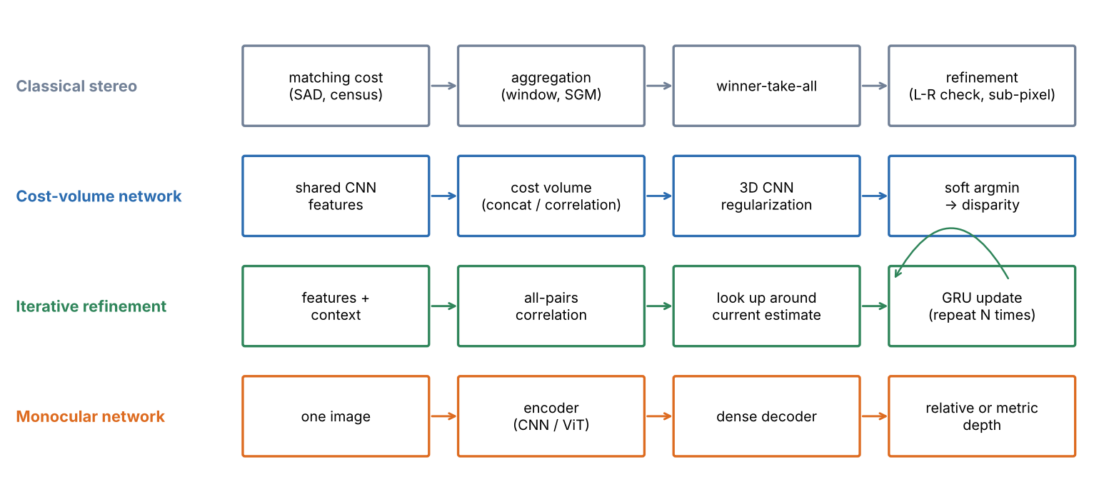
Figure 1 shows the four model families of this tutorial: three match two images, the fourth relies on what it has learned.
Three dense correspondence problems
Plain version. Rectified stereo matches pixels along the same row. Optical flow matches across frames; monocular depth estimates geometry without a second image.
Precise version. Let be two images of pixels and a pixel, with column and row .
- Optical flow is a vector field such that the point seen at in is seen at in . Two unknowns per pixel; the cameras and the scene may both move.
- Stereo disparity is the special case of two cameras that see the scene at the same instant and have been rectified (next section), so that every match lies on the same row: . One unknown per pixel, the disparity , which converts to depth.
- Monocular depth asks for a depth map from alone. No correspondence is available, so the answer comes from learned regularities, and it is only defined up to an unknown scale unless the network has learned metric cues.
- Scene flow asks for the 3D motion of the point seen at each pixel; it combines depth at two times with optical flow (see Scene flow below).
The two-image problems share one structure: a cost that scores a candidate match, a search over candidates, and a way to resolve pixels where the cost is ambiguous.
Stereo geometry: rectification and disparity
Plain version. In a calibrated rectified pair, nearby points have larger disparity. Focal length and camera baseline convert that disparity into depth.
Rectification
For a general pair of cameras, the match of a pixel lies on its epipolar line in the other image (DLCV 11, epipolar geometry). Rectification warps both images with a homography each so that all epipolar lines become horizontal and corresponding lines have the same row index [1]. After rectification the two virtual cameras have the same intrinsics, parallel optical axes and a purely horizontal baseline. Stereo rigs are calibrated once, and every frame is rectified before matching; all the stereo benchmarks below distribute rectified pairs. In the rest of this tutorial the pair is always rectified.
Disparity and depth
Place the left camera centre at the origin and the right camera at distance along the axis (Figure 2a). A point at depth and horizontal position projects to column in the left image and in the right image, both measured from the principal point. Subtracting gives
where is the focal length in pixels, is the baseline (distance between the camera centres, in metres), is the depth along the optical axis and is the disparity in pixels. Depth and disparity are inversely proportional: disparity is an inverse depth, scaled by . Large disparities belong to near objects, and a disparity of zero means a point at infinity.
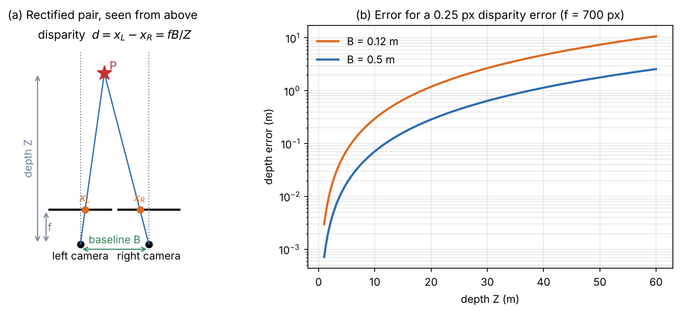
Because , a small disparity error becomes a depth error of about , the same relation that DLCV 11, Triangulation derives. The snippet puts numbers on it for a hypothetical camera with px.
Code · Python · 9 lines
import numpy as np

f = 700.0                                    # focal length in pixels (a hypothetical rig)
for B in [0.12, 0.5]:                        # baselines in metres
    print(f"baseline {B} m: depth at a disparity of 1 px = {f * B:.0f} m")
    for Z in [2, 10, 30, 60]:
        d = f * B / Z                        # disparity in pixels
        dZ = Z ** 2 * 0.25 / (f * B)         # depth error for a 0.25 px disparity error
        print(f"   Z = {Z:2d} m  d = {d:6.2f} px  depth error for 0.25 px: {dZ:6.3f} m ({100 * dZ / Z:4.1f}%)")
Output
baseline 0.12 m: depth at a disparity of 1 px = 84 m
   Z =  2 m  d =  42.00 px  depth error for 0.25 px:  0.012 m ( 0.6%)
   Z = 10 m  d =   8.40 px  depth error for 0.25 px:  0.298 m ( 3.0%)
   Z = 30 m  d =   2.80 px  depth error for 0.25 px:  2.679 m ( 8.9%)
   Z = 60 m  d =   1.40 px  depth error for 0.25 px: 10.714 m (17.9%)
baseline 0.5 m: depth at a disparity of 1 px = 350 m
   Z =  2 m  d = 175.00 px  depth error for 0.25 px:  0.003 m ( 0.1%)
   Z = 10 m  d =  35.00 px  depth error for 0.25 px:  0.071 m ( 0.7%)
   Z = 30 m  d =  11.67 px  depth error for 0.25 px:  0.643 m ( 2.1%)
   Z = 60 m  d =   5.83 px  depth error for 0.25 px:  2.571 m ( 4.3%)
At 10 m, a quarter-pixel disparity error costs 30 cm with a 12 cm baseline and 7 cm with a 50 cm baseline. At 60 m, the short baseline sees a disparity of only 1.4 px and its depth is uncertain by 18%. This is why stereo cameras for driving use wide baselines and high resolution, and why sub-pixel accuracy matters: the last fraction of a pixel decides the far range.
Classical stereo matching
Plain version. Classical block matching searches candidate disparities, compares local patches and refines unreliable matches.
Scharstein and Szeliski organized dense two-frame stereo algorithms into four steps that most methods perform in some form [2]:
- Matching cost computation: a per-pixel, per-disparity dissimilarity.
- Cost (support) aggregation: combine costs over a neighbourhood to reduce noise.
- Disparity computation or optimization: choose a disparity per pixel, either locally or by optimizing an energy over the whole image.
- Disparity refinement: sub-pixel estimates, consistency checks, filling and smoothing.
The Middlebury stereo website, which accompanies that paper, still hosts an online evaluation [2], [3]. The plane sweep in DLCV 11 is exactly steps 1–3 with windowed SSD; here we look at each step more closely and add the refinement.
Matching costs and the cost volume
The simplest cost compares intensities in a small window. The sum of absolute differences (SAD) at pixel and disparity is
where are the left and right images, is the set of offsets of a window centred on the pixel, and ranges over integer hypotheses . Squared differences give SSD. Computing for every pixel and every fills a cost volume of size . The winner-take-all (WTA) rule picks .
SAD assumes both cameras record the same brightness for the same point. Real cameras differ in gain and exposure, so practical systems use zero-mean normalized cross-correlation (ZNCC) or the census transform, which encodes which neighbours are darker than the pixel as a bit string and compares bit strings [4].
Optional: Robust matching costs: ZNCC and census (in the Supplementary notes). The definitions, and a test in which a brightness change between the views breaks SAD but not the other two.
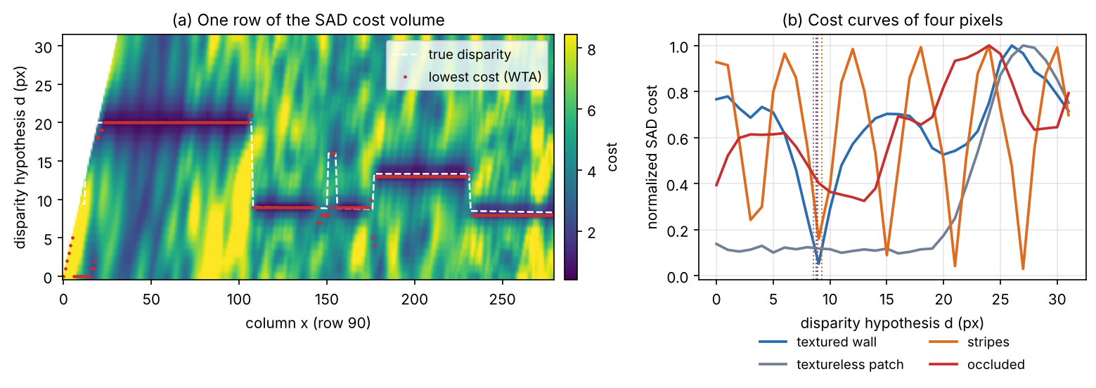
Figure 3a shows one row of a cost volume: dark valleys trace the surfaces. Figure 3b shows four typical cost curves. A textured pixel has one sharp minimum; a textureless pixel a flat curve; a repetitive pattern several equal minima, one per period; and an occluded pixel, hidden in the right image, no correct minimum at all.
Code: block matching with a left–right check
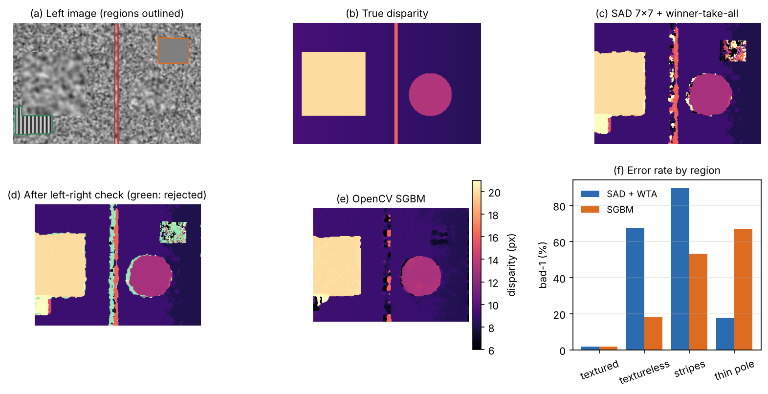
The snippet ray-casts a rectified pair of a synthetic scene with known depth: a slanted textured wall, a box, a disc and a thin pole in front of it, plus a textureless patch and a patch of fine stripes on the wall. It builds the SAD cost volume, takes the WTA disparity, and runs the left–right consistency check: match again with the right image as reference, and reject pixels where the two answers disagree by more than one pixel. Occluded pixels usually fail this check, because their “match” in the right image belongs to a different surface whose own match points elsewhere. For comparison it also runs OpenCV’s semi-global matcher (next subsection). Errors are reported as bad-1, the percentage of pixels whose disparity is off by more than 1 px, separately for each kind of region.
Code · Python · 68 lines
import numpy as np
import cv2
from scipy import ndimage as ndi

rng = np.random.default_rng(0)
H, W, f, B = 180, 280, 320.0, 0.25                    # image size, focal length (px), baseline
tex = ndi.gaussian_filter(rng.random((700, 700)), 1.2)
tex = (tex - tex.min()) / np.ptp(tex)                 # random texture painted on every surface

def render(cx):
    """Ray-cast a rectified camera at (cx, 0, 0) looking down +Z: image, depth Z, region labels."""
    v, u = np.mgrid[0:H, 0:W].astype(float)
    dx, dy = (u - W / 2) / f, (v - H / 2) / f            # ray direction (dx, dy, 1)
    Z = (9 + 0.15 * cx) / (1 - 0.15 * dx)                # slanted wall Z = 9 + 0.15 X
    lab = np.zeros((H, W), int)                          # 0 wall, 1 box, 2 disc, 3 thin pole
    for k, z, inside in [(2, 6.0, lambda X, Y: (X - 1.2) ** 2 + (Y - 0.3) ** 2 < 0.36),
                         (3, 5.0, lambda X, Y: np.abs(X - 0.2) < 0.04),
                         (1, 4.0, lambda X, Y: (np.abs(X + 1.0) < 0.6) & (np.abs(Y) < 0.6))]:
        hit = inside(cx + z * dx, z * dy) & (z < Z)
        Z, lab = np.where(hit, z, Z), np.where(hit, k, lab)
    X, Y = cx + Z * dx, Z * dy
    img = ndi.map_coordinates(tex, [350 + 40 * Y + 60 * lab, 350 + 40 * X], order=1)
    flat = (lab == 0) & (X > 2.2) & (X < 3.6) & (Y > -2.0) & (Y < -0.9)
    rep = (lab == 0) & (X > -3.6) & (X < -2.2) & (Y > 0.9) & (Y < 2.0)
    img[flat] = 0.5                                                  # textureless patch: label 4
    img[rep] = 0.5 + 0.4 * np.sin(2 * np.pi * X[rep] / 0.15)        # repetitive stripes: label 5
    lab[flat], lab[rep] = 4, 5
    return img + rng.normal(0, 0.01, img.shape), Z, lab

left, Z_left, lab = render(0.0)
right, Z_right, _ = render(B)
d_true = f * B / Z_left                                # ground-truth disparity of the left view
rows, cols = np.mgrid[0:H, 0:W]
xr = np.round(cols - d_true).astype(int)               # where each left pixel lands in the right view
occluded = (xr < 0) | (np.abs(Z_right[rows, np.clip(xr, 0, W - 1)] - Z_left) > 0.05)

def sad_volume(ref, other, D, win, sign):
    """cost[d](y, x) = sum over a win x win window of |ref(y, x) - other(y, x - sign*d)|."""
    cost = np.full((D, H, W), np.inf)
    for d in range(D):
        c = ndi.uniform_filter(np.abs(ref - np.roll(other, sign * d, axis=1)), win) * win ** 2
        if sign > 0: c[:, :d] = np.inf                 # no partner pixel exists there
        else:        c[:, W - d:] = np.inf
        cost[d] = c
    return cost

D, win = 32, 7
d_left = sad_volume(left, right, D, win, +1).argmin(0)     # winner-take-all, left image as reference
d_right = sad_volume(right, left, D, win, -1).argmin(0)    # winner-take-all, right image as reference
lr_ok = np.abs(d_left - d_right[rows, np.clip(cols - d_left, 0, W - 1)]) <= 1   # left-right check

sgbm = cv2.StereoSGBM_create(minDisparity=0, numDisparities=D, blockSize=5,
                             P1=8 * 25, P2=32 * 25, uniquenessRatio=0, disp12MaxDiff=-1)
u8 = lambda a: np.clip(a * 255, 0, 255).astype(np.uint8)
d_sgbm = sgbm.compute(u8(left), u8(right)).astype(float) / 16    # OpenCV stores 16 x disparity

valid = ~occluded & (cols >= D)                        # visible in both views, away from the left strip
regions = {"textured": valid & np.isin(lab, [0, 1, 2]), "textureless": valid & (lab == 4),
           "stripes": valid & (lab == 5), "thin pole": valid & (lab == 3)}
bad = lambda d, m: 100 * np.mean(np.abs(d - d_true)[m] > 1)      # % of pixels off by > 1 px
print(f"disparity {d_true.min():.1f}-{d_true.max():.1f} px; occluded: {100 * occluded.mean():.1f}% of pixels")
print("bad-1 (%)          " + "".join(f"{k:>12s}" for k in regions))
for name, d in [("SAD + WTA", d_left), ("OpenCV SGBM", d_sgbm)]:
    print(f"{name:19s}" + "".join(f"{bad(d, m):12.1f}" for m in regions.values()))
print(f"left-right check: keeps {100 * lr_ok[valid].mean():.1f}% of visible pixels, "
      f"rejects {100 * (~lr_ok[occluded]).mean():.1f}% of occluded ones")
kept = valid & lr_ok
print(f"SAD + WTA bad-1 on all visible pixels: {bad(d_left, valid):.1f}% -> after the check {bad(d_left, kept):.1f}%")
Output
disparity 8.3-20.0 px; occluded: 7.7% of pixels
bad-1 (%)              textured textureless     stripes   thin pole
SAD + WTA                   1.8        67.7        89.6        17.4
OpenCV SGBM                 1.7        18.2        53.3        67.2
left-right check: keeps 96.6% of visible pixels, rejects 93.0% of occluded ones
SAD + WTA bad-1 on all visible pixels: 6.1% -> after the check 3.6%
These numbers come from this synthetic scene only. On textured surfaces, SAD block matching is right on 98% of the pixels; in the textureless patch it is wrong on two thirds of them and on the stripes on nine out of ten, as the cost curves predicted. The left–right check rejects 93% of the occluded pixels while keeping 96.6% of the visible ones, and bad-1 on the kept pixels drops from 6.1% to 3.6%. Rejected pixels are holes, not errors: later stages know not to trust them and can fill them from neighbours.
Cost aggregation and semi-global matching
Plain version. Window matching decides each pixel alone. A better rule lets neighbouring pixels “vote”: a pixel in a blank region should take the disparity of its textured neighbours, unless there is good evidence for a depth jump.
The classical way to say this is an energy over the whole disparity map ,
where the second sum runs over pairs of neighbouring pixels , is 1 when the condition holds and 0 otherwise, is a small penalty for a change of one disparity level (slanted surfaces) and is a larger penalty for a jump (depth edges) [5], [6]. Minimizing this energy exactly over a 2D image is intractable in general.
Semi-global matching (SGM) by Hirschmüller [5] approximates it by minimizing the energy along many straight 1D paths through each pixel, each of which can be solved exactly by dynamic programming, and summing the results. Along a path with direction the aggregated cost is
where is the previous pixel on the path and the last term only keeps the numbers bounded [6]. The costs of all directions are summed and WTA picks the disparity, so each pixel receives evidence from far away in many directions at a cost linear in the size of the cost volume. OpenCV’s StereoSGBM is a modified version: by default 5 directions instead of the full algorithm’s 8, small blocks instead of single pixels, and the Birchfield–Tomasi cost instead of mutual information [7].
The snippet shows SGM’s trade-off. In the textureless patch, bad pixels drop from 67.7% to 18.2%, because the smoothness term carries the wall’s disparity into it. But the thin pole, about five pixels wide, is mostly erased (17.4% → 67.2%): it costs two jumps for little evidence (Figure 4e). Neither method resolves the stripes, a genuine ambiguity of the data. Smoothness priors bet that the world is made of large surfaces, and that bet loses on thin structures.
Optional: Semi-global matching step by step (in the Supplementary notes). The recursion along one scanline in code, why , and how two opposite paths fill a textureless gap without blurring a depth step.
Refinement: sub-pixel disparity and post-processing
WTA returns integer disparities, but Figure 2b showed that fractions of a pixel matter. The usual fix fits a parabola through the cost at the best integer disparity and its two neighbours and takes the parabola’s minimum. Further post-processing steps include the left–right check, a median filter and filling of rejected pixels from their neighbours; MC-CNN’s pipeline, for example, combines cross-based aggregation, SGM, a left–right check, sub-pixel enhancement, a median filter and a bilateral filter [6].
Optional: Sub-pixel disparity and the soft argmin (in the Supplementary notes). The parabola formula, and why a learned soft argmin can land between two surfaces at a depth edge.
Learned stereo matching
Plain version. Every step of the classical pipeline has a hand-made rule. Deep stereo replaces them, one at a time, by learned ones: first the cost, then the aggregation, and finally the whole pipeline trained end to end on large synthetic datasets.
The surveys of Laga et al. [8] and Tosi et al. [9] follow the same order as this section: learned parts of the pipeline, then end-to-end networks, then the architectures of the 2020s.
Learning the matching cost
MC-CNN by Žbontar and LeCun [6] trains a convolutional network to decide whether two small patches show the same point, using pairs built from ground-truth disparities as a binary classification set. The network’s output replaces SAD as the matching cost, and the rest of the classical pipeline (cross-based aggregation, SGM, left–right check, sub-pixel enhancement, filtering) follows. The lesson: a learned similarity is far more discriminative than raw intensities, but the hand-made aggregation remained.
End-to-end networks with cost volumes
End-to-end training needs dense ground truth for many images, which real scans rarely give. Mayer et al. [10] rendered three datasets (FlyingThings3D, Monkaa, Driving); FlyingThings3D alone has about 25,000 stereo frames of random objects flying along random 3D paths, and with it they trained DispNet, an encoder–decoder that regresses disparity [10]. Together these “Scene Flow” datasets became the usual pre-training data for stereo networks.
GC-Net by Kendall et al. [11] made the cost volume explicit and learnable. A shared 2D CNN extracts features from both images. For every disparity level the left feature is concatenated with the right feature shifted by that level, which gives a 4D volume of size height × width × (max disparity + 1) × feature size [11]. 3D convolutions over this volume learn the aggregation, using context in space and in disparity. Finally, a soft argmin turns the regularized costs into a sub-pixel disparity:
where is the softmax over the disparity dimension and the largest disparity [11]. Unlike the argmin it is differentiable, so the network trains end to end with a regression loss on . PSMNet [12] added a spatial pyramid pooling module that gathers context at several scales before the cost volume and a stacked-hourglass 3D CNN with intermediate supervision to regularize it, trained with the smooth L1 loss [12]. Both target ill-posed regions such as occlusions, repeated patterns, textureless and reflective surfaces, where local patches carry no answer [12].
The price of 3D convolutions is memory and computation proportional to , so these networks work at reduced resolution and a fixed maximum disparity.
Iterative refinement and zero-shot stereo
RAFT-Stereo [13] adapts the RAFT optical flow network (described in the optical flow section below) to rectified stereo: it replaces RAFT’s 4D all-pairs volume by a 3D volume that only compares pixels on the same row, and refines a disparity field step by step with recurrent units that look up the volume around the current estimate, adding multi-level GRUs that pass information across the image more efficiently [13]. There is no 3D convolution and no fixed disparity range to regularize. Tosi et al. call this design “a game changer”, noting that it brought much higher robustness to domain shift and that most recent frameworks follow it [9]. IGEV-Stereo [14] combines the two ideas: a geometry encoding volume that encodes geometry and context gives the recurrent updates a good starting point and is indexed by them at every iteration [14].
The open problem these surveys emphasized was generalization: networks fine-tuned on one benchmark often fail on another [9], [15]. FoundationStereo [16] targets zero-shot use: it is trained on a large synthetic dataset of about one million stereo pairs with automatic removal of ambiguous samples, and it adapts features from a monocular vision foundation model through a side-tuning backbone to narrow the gap between synthetic and real images [16].
Monocular depth estimation
Plain version. With one image there is nothing to match. A network has to recognize depth the way people do with one eye closed: from perspective, the known sizes of things, occlusion, shading, haze and texture that gets finer with distance. These cues tell you which things are nearer, but they cannot tell a toy car from a real one.
Why one image is not enough: scale ambiguity
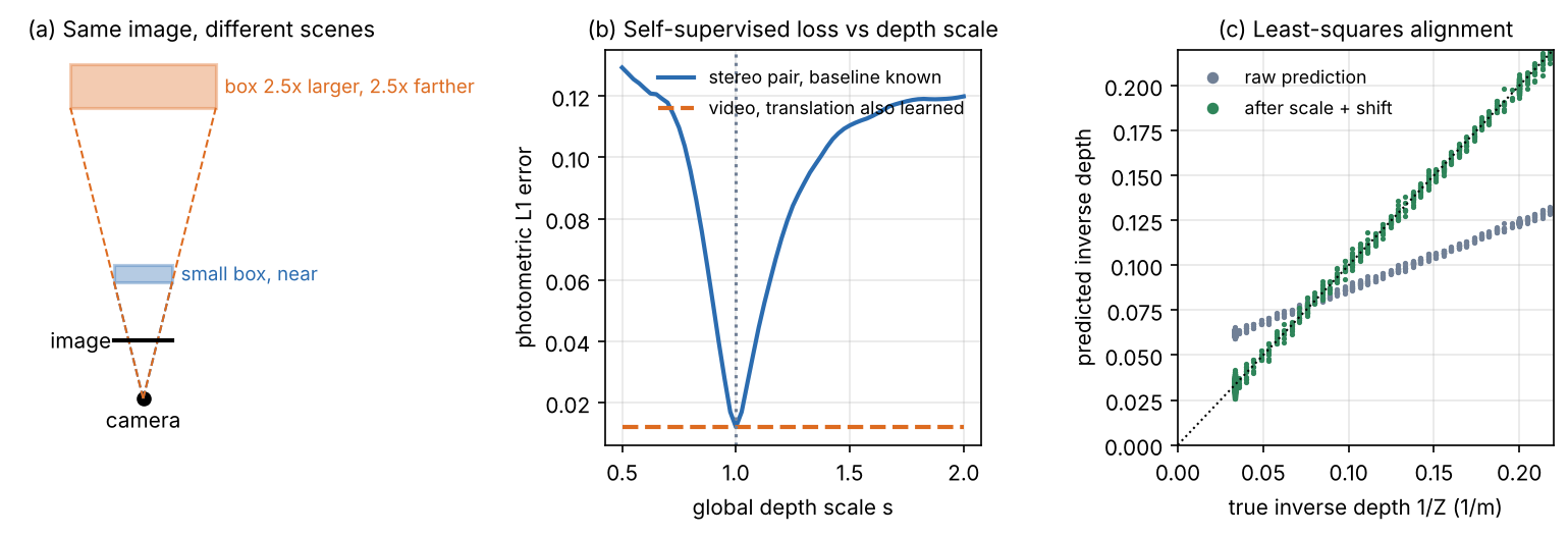
Scale the whole scene by a factor and the image does not change, because projection divides by depth (Figure 5a; see also DLCV 11 and, for 3D detection, DLCV 03B). Eigen et al. called the global scale “a fundamental ambiguity in depth prediction” and showed that much of their error came from the mean depth alone [17].
A network can still learn metric cues, such as typical object sizes or the camera height of a driving dataset, but they fail when the camera or scene type changes. So two kinds of output are used:
- Relative (affine-invariant) depth. The prediction is correct up to an unknown scale and shift. Many such models, MiDaS and Depth Anything among them, predict inverse depth (disparity-like values) [18], [19], so the output satisfies for unknown and . This is enough for ordering, segmentation, editing and many robot tasks when combined with a few metric measurements.
- Metric depth. The prediction is in metres. It requires either a known camera or a model that estimates the camera from the image.
Losses that ignore scale and shift
To train on datasets whose depth is known only up to scale, or in different units, the loss must ignore the unknown factors. Eigen et al. introduced a scale-invariant log error [17]:
where and are the predicted and true depths at pixel , is the number of pixels with ground truth, and is the log-scale offset that best aligns the two maps; multiplying by any constant leaves unchanged [17]. For training they used a blend of this error and the ordinary log-space L2 error, weighted by , which they found gave good absolute-scale predictions [17].
MiDaS by Ranftl et al. [18] went one step further: it predicts inverse depth (disparity) up to scale and shift, and aligns each prediction to the ground truth before computing the loss. With the predicted disparities and the ground truth at the valid pixels, the alignment solves
which is an ordinary least-squares fit of a line with a closed-form solution [18]. The scale-and-shift-invariant loss is then with a per-pixel loss , here the squared error [18]. MiDaS also has a robust variant (median-based alignment, trimmed absolute loss), a gradient-matching term that keeps depth edges sharp, and mixes five training datasets, including one built from 3D films [18]. It is evaluated by zero-shot cross-dataset transfer, on datasets never seen in training [18].
Optional: MiDaS (Ranftl et al., 2022) (in the Paper guides). The problem the paper poses, how its tables are aligned, and what to check before comparing its numbers with others.
The snippet builds a toy depth map (a ground plane, a far wall and a box), simulates a relative model whose output is inverse depth with an unknown scale and shift, and compares three ways of reading it.
Code · Python · 28 lines
import numpy as np

rng = np.random.default_rng(1)
H, W, f, cam_h = 120, 160, 150.0, 1.5
v, u = np.mgrid[0:H, 0:W].astype(float)
Z = np.full((H, W), 30.0)                                      # far wall
below = v > H / 2 + 1
Z[below] = np.minimum(30.0, f * cam_h / (v[below] - H / 2))    # ground plane seen by a camera 1.5 m high
box = (np.abs(u - 50) < 15) & (v > 45) & (v < 80)
Z[box] = 5.0                                                   # an object 5 m away

# A "relative" network outputs inverse depth up to an unknown scale and shift, plus some noise.
pred = 0.37 / Z + 0.05 + rng.normal(0, 0.001, Z.shape)

def metrics(Zp, Zt):
    absrel = np.mean(np.abs(Zp - Zt) / Zt)
    rmse = np.sqrt(np.mean((Zp - Zt) ** 2))
    delta1 = np.mean(np.maximum(Zp / Zt, Zt / Zp) < 1.25)
    return f"AbsRel {absrel:6.3f}   RMSE {rmse:6.2f} m   delta<1.25 {100 * delta1:5.1f}%"

Z_raw = 1 / pred                                               # read the output as if it were metric
Z_med = Z_raw * np.median(Z) / np.median(Z_raw)                # median scaling (scale only)
A = np.c_[pred.ravel(), np.ones(pred.size)]                    # least squares for (s, t) in inverse depth
s, t = np.linalg.lstsq(A, (1 / Z).ravel(), rcond=None)[0]
Z_ssi = 1 / (s * pred + t)
print("raw output        ", metrics(Z_raw, Z))
print("median scaling    ", metrics(Z_med, Z))
print("scale+shift (LSQ) ", metrics(Z_ssi, Z), f"  s = {s:.3f}, t = {t:.4f}")
Output
raw output         AbsRel  0.460   RMSE  10.46 m   delta<1.25  10.2%
median scaling     AbsRel  0.785   RMSE   7.24 m   delta<1.25  54.8%
scale+shift (LSQ)  AbsRel  0.043   RMSE   1.84 m   delta<1.25  99.5%   s = 2.699, t = -0.1348
These are toy numbers. Read as metric depth, the output is useless (δ < 1.25 on 10% of the pixels). Median scaling multiplies the depth by one factor; it helps δ but makes AbsRel worse, because no single factor can undo a shift in inverse depth. The least-squares fit finds , , almost exactly the simulated , and the map becomes nearly perfect. The same prediction can look poor or excellent depending on the alignment, so always check which one a paper used.
From relative to metric foundation models
Modern monocular models use standard dense-prediction networks; the progress came from training data and from how scale is handled. On the relative side, DPT [20] brought a Vision Transformer encoder to dense prediction, Depth Anything [19], [21] scaled training with tens of millions of pseudo-labelled images, and Marigold [22] turned an image diffusion model into a depth estimator. On the metric side, ZoeDepth [23] adds metric heads to a relative model, while Metric3D [24], [25], UniDepth [26] and Depth Pro [27] handle the camera explicitly, by mapping images to a canonical focal length or by estimating the camera from the image. The one idea to remember: relative depth is now robust across many kinds of images, and metric depth becomes usable once the model knows, or can infer, the camera. Dense pointmap models such as DUSt3R and VGGT, which predict geometry and cameras jointly, are covered in DLCV 11, Feed-forward reconstruction.
Optional: Monocular depth foundation models: data and the camera (in the Supplementary notes). What each of these seven models changes, model by model.
Self-supervised depth from stereo pairs and video
Plain version. Instead of ground-truth depth, use a second view as the teacher. If the network’s depth were right, you could warp the second view onto the first and get the same picture. The difference between the warped and the real image is the training signal.
View synthesis as supervision
Garg et al. [28] trained a monocular network on stereo pairs with a known, small camera displacement: the predicted depth of the left image, together with the known baseline, warps the right image into the left view, and the photometric error of this reconstruction is the loss, with no depth labels at all [28]. Godard et al. [29] added a left–right consistency loss that makes the disparities predicted for the two views agree, which improved quality [29]. Zhou et al. [30] removed the second camera: from unlabelled monocular video they trained a depth network and a pose network together, with view synthesis between neighbouring frames as the only supervision [30].
For a target frame and a source frame , each target pixel (in homogeneous coordinates) is mapped to the source by
where is the camera intrinsic matrix, is the predicted depth of the pixel, is the predicted relative camera pose (rotation and translation) and means equality up to the homogeneous scale. Sampling at with a bilinear sampler (DLCV 09A.3) gives the synthesized image ; gradients flow through it into both networks.
Monodepth2
Monodepth2 by Godard et al. [31] showed that a simple model with careful design choices beats more complex ones. Its photometric error between two images combines SSIM (DLCV 09, full-reference metrics) and L1:
where are the target image and a synthesized image, compared per pixel [31], [32]. Three ideas make it robust [31]:
- Per-pixel minimum reprojection. With several source frames (previous and next), take the minimum error over sources instead of the average, , because a pixel occluded in one source is usually visible in the other.
- Auto-masking. Ignore pixels whose error without warping is already lower than with warping. This removes a static camera, and objects that move with the camera, which would otherwise teach the network “infinite depth” for cars driving ahead.
- Full-resolution multi-scale loss. Upsample lower-resolution depth predictions to the input size before computing the error, which reduces artefacts.
An edge-aware smoothness term, weighted by , discourages depth changes where the image itself is smooth [31].
Scale, again
Trained from monocular video, a depth network never sees a metric quantity: depth and translation can be scaled together without changing . Figure 5b shows it on the synthetic stereo scene: with the baseline fixed, the photometric loss has a sharp minimum at the true scale; if the translation scales with the depth, the loss is flat. This is why Monodepth2 reports monocular-trained results after per-image median ground-truth scaling, following SfMLearner, but not for stereo-trained ones, “as scale can be inferred from the known camera baseline” [31]. The other limits are those of matching itself: textureless and reflective surfaces, moving objects and occlusions.
Optical flow as a learning problem
Plain version. Flow is stereo without the rulebook: the match can move in any direction, by a fraction of a pixel or by a hundred pixels, and objects move independently. Classical methods solved an energy for every image pair; deep methods learn to match and refine from synthetic videos.
From energies to networks
The classical methods start from brightness constancy, , which gives one equation for two unknowns per pixel, and add an assumption to resolve it: global smoothness of the flow field (Horn and Schunck [33]), constant flow in a small window solved by least squares (Lucas and Kanade [34]), or a local polynomial model of the image (Farnebäck [35]). DLCV 04B introduces these ideas and the aperture problem.
Optional: Brightness constancy and the classical flow solvers (in DLCV 04B’s Supplementary notes). The linearized flow equation, the Horn–Schunck energy and the polynomial expansion behind Farnebäck’s method.
Hur and Roth [36] describe the move to deep learning in two families: CNNs used as feature extractors inside classical energy formulations, and end-to-end networks that regress the flow directly. The second family won. Four milestones lead to RAFT:
- FlowNet [37] regressed flow end to end with a CNN. Lacking real training data, its authors built Flying Chairs, 22,872 image pairs of rendered 3D chair models moved by random affine transformations over photographs, and found that networks trained on it still generalized to Sintel and KITTI [37]. Its FlowNetC variant added a correlation layer that compares the two images’ features at a range of displacements.
- FlowNet 2.0 [38] stacked several FlowNets, each warping the second image with the current estimate, and showed that the order of the training datasets matters a lot [38].
- SPyNet [39] used a classical image pyramid: at each level one image is warped by the current flow and a small network predicts an update of less than a pixel [39].
- PWC-Net [40] combined pyramid, warping and cost volume on learned features, and is 17 times smaller than FlowNet2 [40].
RAFT: all-pairs correlation and iterative updates
Plain version. RAFT compares every pixel of the first image with every pixel of the second, once. Then it starts from zero motion and, like a person adjusting a sketch, repeatedly looks at the match scores near its current guess and nudges the guess, the same small update applied again and again.
RAFT by Teed and Deng [41] has three parts [41]:
- Features. A CNN encoder maps both images to features at 1/8 resolution with channels; a separate context network encodes the first image only.
- All-pairs correlation. The correlation volume holds the dot product of every feature pair,
where is channel of the feature at row , column , and at feature resolution. Average pooling of the last two dimensions with kernels 1, 2, 4 and 8 gives a four-level correlation pyramid, which keeps full resolution for the first image and covers large displacements in the coarse levels. 3. Iterative updates. Starting from , a convolutional GRU (gated recurrent unit) repeatedly reads the correlation values in a small neighbourhood (radius ) around the position each pixel currently points to, at all pyramid levels, together with the context features and the current flow, and outputs an update: . The weights are shared across iterations. A learned convex upsampling turns the 1/8-resolution flow into full resolution.
The loss supervises every iterate with exponentially increasing weight,
where is the upsampled flow after update , is the number of updates and the ground truth [41]. RAFT unrolls 12 updates in training and can run more at test time; the paper evaluates after 32 updates on Sintel and 24 on KITTI [41]. Training follows the standard schedule: Flying Chairs, then FlyingThings3D, then fine-tuning on the target benchmark [41].
Why did this design win? The all-pairs volume avoids a weakness of coarse-to-fine schemes, which can lose a small fast object at a coarse level for good [41]; the shared update behaves like a learned optimizer; and the recipe transferred to stereo [13] and scene flow [42].
Optional: RAFT (Teed and Deng, 2020) (in the Paper guides). How to read RAFT’s ablations and its benchmark tables.
After RAFT
Later models change one part of the recipe. GMFlow [43] and Unimatch [44] replace iterative lookups by global matching with Transformer features: every pixel is compared with all pixels of the other image and the flow is the softmax-weighted average position; Unimatch uses one model for flow, stereo and depth from posed images [44]. FlowFormer [45] encodes RAFT’s cost volume with transformer layers. SEA-RAFT [46] keeps RAFT but adds a mixture-of-Laplace loss, a directly regressed initial flow and rigid-motion pre-training, for speed and better generalization [46].
Code: measuring flow errors
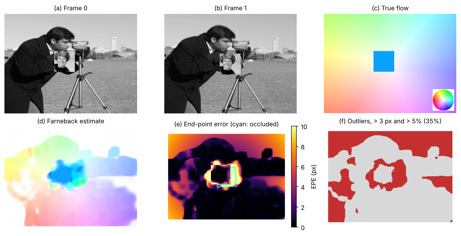
The snippet builds a pair of frames with known flow: the background (the camera test image) rotates by 2° and zooms by 3% about the centre, and a textured patch moves by (14, 6) pixels on top of it. It runs OpenCV’s Farnebäck flow with one and with four pyramid levels and reports the end-point error (EPE, the length of the error vector) and the Fl outlier rate used by KITTI (defined in Evaluation) on different kinds of pixels.
Code · Python · 49 lines
import numpy as np
import cv2
from scipy import ndimage as ndi
from skimage import color, data, transform

I0 = transform.resize(data.camera() / 255.0, (240, 320), anti_aliasing=True)
H, W = I0.shape
rows, cols = np.mgrid[0:H, 0:W].astype(float)
cy, cx = H / 2, W / 2

# Ground-truth motion from frame 0 to frame 1: the background rotates by 2 degrees and zooms by 3 %
# about the image centre; a 50 x 50 textured patch moves by (dx, dy) = (14, 6) pixels.
a, s = np.deg2rad(2.0), 1.03
bx = cx + s * (np.cos(a) * (cols - cx) - np.sin(a) * (rows - cy))     # where each background pixel goes
by = cy + s * (np.sin(a) * (cols - cx) + np.cos(a) * (rows - cy))
flow = np.stack([bx - cols, by - rows], -1)
patch = transform.resize(color.rgb2gray(data.astronaut())[30:230, 150:350], (50, 50), anti_aliasing=True)
obj0 = (rows >= 90) & (rows < 140) & (cols >= 120) & (cols < 170)
flow[obj0] = (14.0, 6.0)

# Render frame 1 by backward mapping (inverse rotation and zoom), then paste the moved patch.
xs = cx + (np.cos(a) * (cols - cx) + np.sin(a) * (rows - cy)) / s
ys = cy + (-np.sin(a) * (cols - cx) + np.cos(a) * (rows - cy)) / s
I1 = ndi.map_coordinates(I0, [ys, xs], order=3, mode="reflect")
I0 = I0.copy(); I0[90:140, 120:170] = patch
I1[96:146, 134:184] = patch
# occluded: background points of frame 0 that land under the patch in frame 1
occ = ~obj0 & (by >= 96) & (by < 146) & (bx >= 134) & (bx < 184)

def evaluate(est, mask):
    epe = np.linalg.norm(est - flow, axis=-1)[mask]
    mag = np.linalg.norm(flow, axis=-1)[mask]
    fl = np.mean((epe > 3) & (epe > 0.05 * mag))       # KITTI outlier: > 3 px and > 5 % of the true motion
    return f"EPE {epe.mean():5.2f} px  Fl {100 * fl:5.1f}%"

u8 = lambda im: (np.clip(im, 0, 1) * 255).round().astype(np.uint8)
inner = np.zeros((H, W), bool); inner[10:-10, 10:-10] = True
grad = ndi.gaussian_filter(np.hypot(ndi.sobel(I0, 0), ndi.sobel(I0, 1)), 4)
bg = inner & ~obj0 & ~occ
flat = grad < 0.05                                     # almost no texture (mostly the sky)
for levels in [1, 4]:
    est = cv2.calcOpticalFlowFarneback(u8(I0), u8(I1), None, pyr_scale=0.5, levels=levels, winsize=15,
                                       iterations=5, poly_n=7, poly_sigma=1.5, flags=0)
    print(f"Farneback, {levels} pyramid level(s):")
    for name, m in [("background, textured", bg & ~flat), ("background, flat", bg & flat),
                    ("moving patch", obj0), ("occluded", occ), ("all (Fl-all)", inner)]:
        print(f"   {name:21s} {evaluate(est, m)}")
print(f"true motion: background up to {np.linalg.norm(flow[~obj0], axis=-1).max():.1f} px, patch "
      f"{np.hypot(14, 6):.1f} px; occluded pixels: {occ.sum()}")
Output
Farneback, 1 pyramid level(s):
   background, textured  EPE  0.87 px  Fl   9.3%
   background, flat      EPE  5.51 px  Fl  90.3%
   moving patch          EPE 18.24 px  Fl 100.0%
   occluded              EPE  5.07 px  Fl  68.0%
   all (Fl-all)          EPE  2.86 px  Fl  35.6%
Farneback, 4 pyramid level(s):
   background, textured  EPE  1.18 px  Fl  11.9%
   background, flat      EPE  5.52 px  Fl  90.5%
   moving patch          EPE  2.30 px  Fl  30.4%
   occluded              EPE 12.20 px  Fl  99.8%
   all (Fl-all)          EPE  2.55 px  Fl  35.2%
true motion: background up to 9.3 px, patch 15.2 px; occluded pixels: 871
These numbers are from this toy pair only. With one level, the patch’s 15 px motion is out of reach and every patch pixel is an outlier; with four levels the patch is found (EPE 2.30 px), the coarse-to-fine idea of SPyNet and PWC-Net in classical form. Two failures remain. In flat regions (mostly the sky) 90% of the pixels are outliers: there is nothing to match. On occluded pixels, the strip the patch covers in frame 1, the pyramid makes things worse (EPE 12.2 px), because the coarse levels drag them along with the patch (Figure 6). Learned methods are trained to handle both cases from data, but neither disappears.
Scene flow in brief
Plain version. Optical flow says how a point moves in the image. Scene flow says how it moves in 3D: closer, farther, left or right, in metres.
Scene flow is the dense 3D motion field of the scene, a term that goes back to Vedula et al. [47]; optical flow is its projection onto the image. RAFT-3D states the task as: given a pair of stereo or RGB-D video frames, estimate the 3D motion of every pixel [42]. With a stereo camera it can be estimated from the disparity at two times plus the optical flow between them. The KITTI 2015 benchmark by Menze and Geiger [48] evaluates exactly these parts: D1 (disparity in the first frame), D2 (disparity in the second frame), Fl (optical flow) and SF, which counts a pixel as wrong if any of the three is wrong [49]. Menze and Geiger modelled the scene as a small number of rigidly moving objects, with each superpixel a 3D plane assigned to one of them [48]; RAFT-3D [42] instead estimates a dense field of rigid 3D motions with RAFT-style iterations and groups pixels softly into rigid objects with learned embeddings [42]. Dynamic reconstruction (DLCV 11) and point tracking (DLCV 07) are its long-range relatives.
Evaluation
Plain version. All three tasks are scored per pixel against ground truth, with an average error and a “percentage of bad pixels”. The details, especially how monocular predictions are aligned and which pixels count, change the numbers more than you would expect.
Depth metrics
The standard set goes back to Eigen et al. [17]. With the predicted and the true depth at the evaluated pixels,
plus RMSE of [17]. AbsRel, SqRel and RMSE are errors (lower is better); with are accuracies (higher is better). AbsRel weights near and far pixels by their relative error; RMSE is dominated by far pixels; counts pixels within 25% of the truth.
State three conventions with every result: the alignment (none for metric models, per-image median scaling for self-supervised monocular ones [31], least-squares scale and shift for affine-invariant ones [18]); the depth cap (80 m is standard on KITTI [31]); and the split (often that of Eigen et al. on KITTI [17], [31]). The alignment snippet showed how much the first one alone changes.
Stereo metrics
- EPE (mean absolute disparity error, in pixels).
- bad-τ: percentage of pixels with a disparity error larger than pixels. Middlebury’s Version 3 evaluation reports bad 2.0 by default, on all or only non-occluded pixels [3]; KITTI 2012 reports the percentage of erroneous pixels at thresholds from 2 to 5 pixels, in non-occluded areas (Out-Noc) and in total (Out-All) [50].
- D1 (KITTI 2015): a pixel’s disparity is correct if its error is below 3 px or below 5% of the true value; D1 is the percentage of outliers, reported over background, foreground or all pixels (D1-bg, D1-fg, D1-all) [49]. The relative clause keeps near objects, with large disparities, from being judged too harshly.
Flow metrics
- EPE: the mean Euclidean distance between estimated and true flow vectors, , where and are the estimated and true flow at pixel ; FlowNet calls it the standard error measure for optical flow and also trains with it [37]. Sintel results are reported as average EPE (often written AEPE).
- Fl-all (KITTI 2015): the percentage of pixels whose end-point error is at least 3 px and at least 5% of the true flow length, over all pixels with ground truth [49]. The snippet’s
evaluatefunction computes exactly this.
Datasets and benchmarks
| Dataset | Task | What it contains | Ground truth |
|---|---|---|---|
| KITTI 2012 [51], [50] | stereo, flow | 194 training and 195 test pairs of real road scenes | sparse, from a laser scanner |
| KITTI 2015 [48], [49] | stereo, flow, scene flow | 200 training and 200 test scenes with moving cars | sparse, semi-automatic, with 3D CAD models fitted to moving vehicles |
| Middlebury 2014 [52] | stereo | 33 high-resolution indoor scenes; 20 used in the Version 3 evaluation (10 training, 10 test) | dense, subpixel-accurate |
| ETH3D [53] | stereo, multi-view stereo | indoor and outdoor scenes with DSLR images and low-resolution stereo videos; includes a low-resolution two-view benchmark | high-precision laser scans |
| MPI Sintel [54] | flow (also stereo, depth) | frames of an open-source animated film; “clean” and “final” passes, the final one with motion blur and atmospheric effects | dense, rendered |
| Flying Chairs [37] | flow (training) | 22,872 synthetic image pairs | dense, rendered |
| FlyingThings3D [10] | stereo, flow, scene flow (training) | about 25,000 synthetic stereo frames at 960 × 540 | dense, rendered |
| NYU Depth v2 [55] | monocular depth (indoor) | Kinect video of 464 indoor scenes; 1,449 densely labelled RGB-D pairs | dense, from the Kinect depth camera, missing values filled in |
Sizes and ground-truth types come from the cited pages and papers; the description of Sintel’s two passes is from [37], and KITTI 2015’s semi-automatic ground truth from [49], [48]. The synthetic sets are used for pre-training, the real ones for fine-tuning and testing.
Failure modes
Plain version. Every method in this tutorial relies on one of two things: something to match, or a prior learned from training data. Each failure below breaks one of them.
- Textureless regions (white walls, sky, road): flat matching costs (Figure 3b), filled by smoothness or learned context, both possibly wrong.
- Repetitive patterns (fences, tiles): several disparities fit equally well, as the stripes showed.
- Reflective and transparent surfaces: the matched content is a reflection or the scene behind. Tosi et al. count transparent and reflective objects among the four main open challenges of deep stereo, with domain shift, over-smoothing and asymmetric stereo pairs [9].
- Occlusions: no correct match exists; they need detection (left–right check) and filling, and in flow they are dragged along with neighbouring motion.
- Thin structures and depth edges: windows fatten foreground objects, smoothness erases poles and wires, and a soft argmin over a two-peaked cost lands between surfaces.
- Large motion of small objects: coarse-to-fine schemes can lose them; RAFT’s all-pairs volume targets this [41].
- Domain gap: models pre-trained on synthetic data and fine-tuned on one benchmark degrade on new cameras, weather and scenes [9], [36].
- Scale and the camera (monocular): relative depth has no scale, and metric depth fails when the focal length is unknown or the image has been cropped unexpectedly.
- Moving objects in self-supervision break the static-scene assumption; auto-masking handles only the simplest cases [31]. Rajapaksha et al. add thin, small and distant objects to the open gaps of monocular depth [56].
Modern view
What the surveys say
Five reviews cover the ground of this tutorial. Laga et al. [8] survey deep stereo (two-view and multi-view) up to about 2019, split into methods that learn parts of the classical pipeline and end-to-end pipelines, with datasets and supervision modes; monocular depth is outside their scope. Poggi et al. [15] stress that learning and stereo help each other: learning improves stereo, and stereo supervises monocular networks; they also cover confidence estimation and domain shift. Tosi et al. [9] review the 2020s: architectures grouped into cost volume aggregation, neural architecture search, iterative optimization, Vision Transformers and Markov random fields, and four open challenges (domain shift, over-smoothing, transparent and reflective objects, asymmetric stereo); in 2024 they noted that a stereo foundation model was still missing. Rajapaksha et al. [56] organize monocular depth by input and output, architecture and degree of supervision. Hur and Roth [36] trace optical flow from energy minimization to CNNs and name domain overfitting and complex training schedules as the main limits.
Optional: Guide to the Modern view surveys (in the Paper guides). Which survey to read for which question, and what each one does not cover.
The state of the art, 2023–2026
- Foundation models for monocular depth. Large-scale data (Depth Anything [19], [21]), generative priors (Marigold [22]) and explicit camera handling (Metric3D [24], [25], UniDepth [26], Depth Pro [27]) made zero-shot depth from arbitrary photos practical, first relative and now increasingly metric.
- Iterative matching for stereo and flow. The RAFT recipe of a correlation volume plus recurrent updates dominates both tasks [9]; recent variants add geometry volumes (IGEV-Stereo [14]), global matching with attention (GMFlow, Unimatch [43], [44]) or simpler training (SEA-RAFT [46]).
- Zero-shot stereo. FoundationStereo [16] answered the missing-foundation-model point of Tosi et al. by combining a million synthetic pairs with monocular priors.
- Convergence with 3D reconstruction. Feed-forward models that predict pointmaps and cameras (DLCV 11) blur the line between depth estimation, stereo and structure from motion.
Open problems
- Metric depth in the wild: unknown, cropped or unusual cameras, and a reliable uncertainty for each prediction.
- Non-Lambertian scenes: glass, mirrors and water for both stereo and flow [9].
- Sharp boundaries and thin structures without over-smoothing or “flying pixels” between surfaces.
- Temporal consistency: per-frame depth flickers in video; flow and depth over long sequences should agree with each other.
- Evaluation: sparse or semi-automatic ground truth, differing alignment conventions and benchmark saturation make small differences hard to interpret.
Key takeaways
- Rectified stereo constrains matches to image rows; flow searches across time; monocular depth relies on learned or geometric assumptions.
- Depth sensitivity increases as disparity shrinks; calibration, baseline and sub-pixel precision limit usable range.
- Cost aggregation and regularization fill uncertain regions but can erase thin structures.
- Distinguish relative from metric depth and state any scale or shift alignment used in evaluation.
- Photometric supervision depends on visibility and scene assumptions; moving or occluded content needs special handling.
- Report error units, evaluated pixels, depth caps and splits; comparable model names do not imply comparable protocols.
Exercises
- Choose a baseline. A stereo camera with px must measure depth at 40 m with an error below 1 m, assuming a disparity error of 0.3 px. What is the smallest baseline? What disparity does a point at 40 m then have, and what happens at 80 m?
Hint
From : m. The disparity at 40 m is px. At 80 m the error is four times larger (about 4 m) and the disparity is 6 px.
- Window size and fattening. In the block-matching snippet, change
winto 3, 7 and 15 and compare bad-1 on the four regions. Why does a large window help in one place and hurt in another?
Hint
In our run, textureless bad-1 fell from 84.4% (3 × 3) to 67.7% (7 × 7) and 39.9% (15 × 15), while the thin pole rose from 15.3% to 17.4% and 74.6%. A large window gathers texture from outside the flat patch, but near depth edges it mixes two surfaces and spreads the foreground disparity into the background (“foreground fattening”), which swallows the pole.
- Stripes and the period. The stripes on the wall have a period of 0.15 world units, and the wall there is about 8.6 units away. Estimate their period in pixels (use px), then explain why block matching gives wrong disparities there. Which change to the scene would make the stripes matchable, and which change to the algorithm might help?
Hint
The period is about px, smaller than the true disparity there (about 9.3 px), so shifts that differ by one period fit equally well. A wider search does not help. Non-periodic texture would; a smoothness term that prefers the surrounding wall’s disparity reduces the errors (in our run SGBM’s bad-1 on the stripes was 53.3% against 89.6% for block matching) but does not remove them.
- Scale-invariant losses by hand. Show that Eigen’s error does not change when is multiplied by a constant . Then show that MiDaS’s least-squares makes unchanged under for any and .
Hint
, and absorbs , so every residual is unchanged. For MiDaS, if is optimal for , then gives the same aligned values for .
- Pyramids and large motion. In the flow snippet, move the patch by (24, 10) instead of (14, 6) and run with 1, 4 and 6 pyramid levels; then move it by only (2, 1). Update the pasted position in frame 1 and the occlusion mask too. When does the pyramid help?
Hint
In our run, at (24, 10) the patch was lost with every setting (EPE about 26 px), and 6 levels gave exactly the same result as 4, so the extra levels added nothing here. At (2, 1) all three settings gave a patch EPE of 0.27 px. A pyramid helps only for motions that its coarse levels can bring within reach of the local model; beyond that, a different search is needed, such as RAFT’s all-pairs correlation.
References
- R. Hartley and A. Zisserman, Multiple View Geometry in Computer Vision, 2nd ed., Cambridge University Press, 2004. doi
- D. Scharstein and R. Szeliski, “A taxonomy and evaluation of dense two-frame stereo correspondence algorithms,” International Journal of Computer Vision, vol. 47, no. 1–3, pp. 7–42, 2002. doi
- D. Scharstein, R. Szeliski and H. Hirschmüller, “Middlebury Stereo Evaluation — Version 3,” official benchmark page (bad 2.0 metric, non-occluded and all masks). link · stereo home page
- R. Zabih and J. Woodfill, “Non-parametric local transforms for computing visual correspondence,” in Computer Vision — ECCV ‘94 (Lecture Notes in Computer Science), pp. 151–158, Springer, 1994. doi
- H. Hirschmüller, “Stereo processing by semiglobal matching and mutual information,” IEEE Transactions on Pattern Analysis and Machine Intelligence, vol. 30, no. 2, pp. 328–341, 2008. doi
- J. Žbontar and Y. LeCun, “Stereo matching by training a convolutional neural network to compare image patches,” Journal of Machine Learning Research, vol. 17, no. 65, pp. 1–32, 2016. JMLR · arXiv
- OpenCV contributors, “cv::StereoSGBM class documentation,” OpenCV source,
modules/calib3d/include/opencv2/calib3d.hpp(4.x branch). source - H. Laga, L. V. Jospin, F. Boussaid and M. Bennamoun, “A survey on deep learning techniques for stereo-based depth estimation,” IEEE Transactions on Pattern Analysis and Machine Intelligence, vol. 44, no. 4, pp. 1738–1764, 2022. doi · arXiv
- F. Tosi, L. Bartolomei and M. Poggi, “A survey on deep stereo matching in the twenties,” International Journal of Computer Vision, vol. 133, no. 7, pp. 4245–4276, 2025. doi · arXiv
- N. Mayer, E. Ilg, P. Häusser, P. Fischer, D. Cremers, A. Dosovitskiy and T. Brox, “A large dataset to train convolutional networks for disparity, optical flow, and scene flow estimation,” in Proc. IEEE CVPR, pp. 4040–4048, 2016. CVF · doi
- A. Kendall, H. Martirosyan, S. Dasgupta, P. Henry, R. Kennedy, A. Bachrach and A. Bry, “End-to-end learning of geometry and context for deep stereo regression,” in Proc. IEEE ICCV, 2017. CVF
- J.-R. Chang and Y.-S. Chen, “Pyramid stereo matching network,” in Proc. IEEE/CVF CVPR, 2018. CVF
- L. Lipson, Z. Teed and J. Deng, “RAFT-Stereo: Multilevel recurrent field transforms for stereo matching,” in Proc. International Conference on 3D Vision (3DV), pp. 218–227, 2021. doi · arXiv
- G. Xu, X. Wang, X. Ding and X. Yang, “Iterative geometry encoding volume for stereo matching,” in Proc. IEEE/CVF CVPR, 2023. CVF
- M. Poggi, F. Tosi, K. Batsos, P. Mordohai and S. Mattoccia, “On the synergies between machine learning and binocular stereo for depth estimation from images: A survey,” IEEE Transactions on Pattern Analysis and Machine Intelligence, 2021. doi · arXiv
- B. Wen, M. Trepte, J. Aribido, J. Kautz, O. Gallo and S. Birchfield, “FoundationStereo: Zero-shot stereo matching,” in Proc. IEEE/CVF CVPR, 2025. CVF · arXiv
- D. Eigen, C. Puhrsch and R. Fergus, “Depth map prediction from a single image using a multi-scale deep network,” in Proc. NeurIPS, 2014. proceedings · arXiv
- R. Ranftl, K. Lasinger, D. Hafner, K. Schindler and V. Koltun, “Towards robust monocular depth estimation: Mixing datasets for zero-shot cross-dataset transfer,” IEEE Transactions on Pattern Analysis and Machine Intelligence, vol. 44, no. 3, pp. 1623–1637, 2022. doi · arXiv
- L. Yang, B. Kang, Z. Huang, X. Xu, J. Feng and H. Zhao, “Depth Anything: Unleashing the power of large-scale unlabeled data,” in Proc. IEEE/CVF CVPR, 2024. CVF · arXiv
- R. Ranftl, A. Bochkovskiy and V. Koltun, “Vision transformers for dense prediction,” in Proc. IEEE/CVF ICCV, 2021. CVF
- L. Yang, B. Kang, Z. Huang, Z. Zhao, X. Xu, J. Feng and H. Zhao, “Depth Anything V2,” in Proc. NeurIPS, 2024. proceedings · arXiv
- B. Ke, A. Obukhov, S. Huang, N. Metzger, R. C. Daudt and K. Schindler, “Repurposing diffusion-based image generators for monocular depth estimation,” in Proc. IEEE/CVF CVPR, 2024. CVF · arXiv
- S. F. Bhat, R. Birkl, D. Wofk, P. Wonka and M. Müller, “ZoeDepth: Zero-shot transfer by combining relative and metric depth,” arXiv:2302.12288, 2023. arXiv
- W. Yin, C. Zhang, H. Chen, Z. Cai, G. Yu, K. Wang, X. Chen and C. Shen, “Metric3D: Towards zero-shot metric 3D prediction from a single image,” in Proc. IEEE/CVF ICCV, 2023. CVF · arXiv
- M. Hu, W. Yin, C. Zhang, Z. Cai, X. Long, K. Wang, H. Chen, G. Yu, C. Shen and S. Shen, “Metric3D v2: A versatile monocular geometric foundation model for zero-shot metric depth and surface normal estimation,” IEEE Transactions on Pattern Analysis and Machine Intelligence, vol. 46, no. 12, pp. 10579–10596, 2024. doi · arXiv
- L. Piccinelli, Y.-H. Yang, C. Sakaridis, M. Segu, S. Li, L. Van Gool and F. Yu, “UniDepth: Universal monocular metric depth estimation,” in Proc. IEEE/CVF CVPR, 2024. CVF · arXiv
- A. Bochkovskii, A. Delaunoy, H. Germain, M. Santos, Y. Zhou, S. R. Richter and V. Koltun, “Depth Pro: Sharp monocular metric depth in less than a second,” in Proc. ICLR, 2025. OpenReview · arXiv
- R. Garg, V. Kumar B.G., G. Carneiro and I. Reid, “Unsupervised CNN for single view depth estimation: Geometry to the rescue,” in Proc. ECCV (Lecture Notes in Computer Science), pp. 740–756, 2016. doi · arXiv
- C. Godard, O. Mac Aodha and G. J. Brostow, “Unsupervised monocular depth estimation with left-right consistency,” in Proc. IEEE CVPR, 2017. CVF
- T. Zhou, M. Brown, N. Snavely and D. G. Lowe, “Unsupervised learning of depth and ego-motion from video,” in Proc. IEEE CVPR, 2017. CVF
- C. Godard, O. Mac Aodha, M. Firman and G. J. Brostow, “Digging into self-supervised monocular depth estimation,” in Proc. IEEE/CVF ICCV, 2019. CVF · arXiv
- Z. Wang, A. C. Bovik, H. R. Sheikh and E. P. Simoncelli, “Image quality assessment: From error visibility to structural similarity,” IEEE Transactions on Image Processing, vol. 13, no. 4, pp. 600–612, 2004. doi
- B. K. P. Horn and B. G. Schunck, “Determining optical flow,” Artificial Intelligence, vol. 17, no. 1–3, pp. 185–203, 1981. doi
- B. D. Lucas and T. Kanade, “An iterative image registration technique with an application to stereo vision,” in Proc. International Joint Conference on Artificial Intelligence (IJCAI), 1981. pdf
- G. Farnebäck, “Two-frame motion estimation based on polynomial expansion,” in Image Analysis (Lecture Notes in Computer Science), pp. 363–370, Springer, 2003. doi
- J. Hur and S. Roth, “Optical flow estimation in the deep learning age,” in Modelling Human Motion, N. Noceti, A. Sciutti and F. Rea, Eds., pp. 119–140, Springer, 2020. doi · arXiv
- A. Dosovitskiy, P. Fischer, E. Ilg, P. Häusser, C. Hazırbaş, V. Golkov, P. van der Smagt, D. Cremers and T. Brox, “FlowNet: Learning optical flow with convolutional networks,” in Proc. IEEE ICCV, 2015. CVF · arXiv
- E. Ilg, N. Mayer, T. Saikia, M. Keuper, A. Dosovitskiy and T. Brox, “FlowNet 2.0: Evolution of optical flow estimation with deep networks,” in Proc. IEEE CVPR, 2017. CVF
- A. Ranjan and M. J. Black, “Optical flow estimation using a spatial pyramid network,” in Proc. IEEE CVPR, 2017. CVF
- D. Sun, X. Yang, M.-Y. Liu and J. Kautz, “PWC-Net: CNNs for optical flow using pyramid, warping, and cost volume,” in Proc. IEEE/CVF CVPR, 2018. CVF
- Z. Teed and J. Deng, “RAFT: Recurrent all-pairs field transforms for optical flow,” in Proc. ECCV (Lecture Notes in Computer Science), pp. 402–419, 2020. doi · arXiv
- Z. Teed and J. Deng, “RAFT-3D: Scene flow using rigid-motion embeddings,” in Proc. IEEE/CVF CVPR, 2021. CVF · arXiv
- H. Xu, J. Zhang, J. Cai, H. Rezatofighi and D. Tao, “GMFlow: Learning optical flow via global matching,” in Proc. IEEE/CVF CVPR, 2022. CVF
- H. Xu, J. Zhang, J. Cai, H. Rezatofighi, F. Yu, D. Tao and A. Geiger, “Unifying flow, stereo and depth estimation,” IEEE Transactions on Pattern Analysis and Machine Intelligence, vol. 45, no. 11, pp. 13941–13958, 2023. doi · arXiv
- Z. Huang, X. Shi, C. Zhang, Q. Wang, K. C. Cheung, H. Qin, J. Dai and H. Li, “FlowFormer: A transformer architecture for optical flow,” in Proc. ECCV (Lecture Notes in Computer Science), pp. 668–685, 2022. doi · arXiv
- Y. Wang, L. Lipson and J. Deng, “SEA-RAFT: Simple, efficient, accurate RAFT for optical flow,” in Proc. ECCV (Lecture Notes in Computer Science), pp. 36–54, 2024. doi · arXiv
- S. Vedula, S. Baker, P. Rander, R. Collins and T. Kanade, “Three-dimensional scene flow,” in Proc. IEEE ICCV, vol. 2, pp. 722–729, 1999. doi
- M. Menze and A. Geiger, “Object scene flow for autonomous vehicles,” in Proc. IEEE CVPR, pp. 3061–3070, 2015. CVF · doi
- A. Geiger, P. Lenz, C. Stiller and R. Urtasun, “Scene flow evaluation 2015 (stereo 2015, flow 2015, scene flow 2015),” The KITTI Vision Benchmark Suite, official benchmark page (dataset size, D1, D2, Fl and SF outlier definitions). link
- A. Geiger, P. Lenz, C. Stiller and R. Urtasun, “Stereo evaluation 2012,” The KITTI Vision Benchmark Suite, official benchmark page (dataset size, Out-Noc and Out-All at 2–5 px). link
- A. Geiger, P. Lenz and R. Urtasun, “Are we ready for autonomous driving? The KITTI vision benchmark suite,” in Proc. IEEE CVPR, pp. 3354–3361, 2012. doi
- D. Scharstein, H. Hirschmüller, Y. Kitajima, G. Krathwohl, N. Nešić, X. Wang and P. Westling, “High-resolution stereo datasets with subpixel-accurate ground truth,” in Pattern Recognition (Proc. GCPR) (Lecture Notes in Computer Science), pp. 31–42, Springer, 2014. doi · datasets
- T. Schöps, J. L. Schönberger, S. Galliani, T. Sattler, K. Schindler, M. Pollefeys and A. Geiger, “A multi-view stereo benchmark with high-resolution images and multi-camera videos,” in Proc. IEEE CVPR, pp. 2538–2547, 2017. CVF · datasets
- D. J. Butler, J. Wulff, G. B. Stanley and M. J. Black, “A naturalistic open source movie for optical flow evaluation,” in Proc. ECCV (Lecture Notes in Computer Science), pp. 611–625, 2012. doi · project page
- N. Silberman, D. Hoiem, P. Kohli and R. Fergus, “Indoor segmentation and support inference from RGBD images,” in Proc. ECCV (Lecture Notes in Computer Science), pp. 746–760, 2012. doi · dataset page
- U. Rajapaksha, F. Sohel, H. Laga, D. Diepeveen and M. Bennamoun, “Deep learning-based depth estimation methods from monocular image and videos: A comprehensive survey,” ACM Computing Surveys, vol. 56, no. 12, 2024. doi · arXiv
Check your understanding
This tutorial has 5 exercises. Can you solve them without opening the hints?
Go to the exercises ↑Next DLCV 12 · Image Generation: From GANs to Text-to-Image Systems · 36 min