DLCV 09A.1 · Blind and Real-World Image Super-Resolution
Needs: DLCV 09A · Non-Blind Image Super-Resolution, DLCV 09B · Generative Image Restoration: Sampling a Plausible Answer
Navigate: this page and this track: Navigate: this page and this track
On this page
- What you’ll learn1 min
- The big picture2 min
- The problem: damage nobody measured2 min
- A map of the field3 min
- Explicit degradation modelling5 min
- Degradation representation learning1 min
- Implicit modelling by degradation synthesis3 min
- Real paired and unpaired data2 min
- Real-world SR with generative priors5 min
- Evaluation in the blind and real-world setting5 min
- Failure modes1 min
- Modern view3 min
- Key takeaways1 min
- Exercises3 min
- Supplementary notes
- Paper guides
- References
- SRMD: one network for many known degradations (CVPR 2018)
- IKC: iterative kernel correction (CVPR 2019)
- KernelGAN: kernel estimation with an internal GAN (NeurIPS 2019)
- DAN: unfolding the alternating optimization (NeurIPS 2020)
- DASR: contrastive degradation representations (CVPR 2021)
- BSRGAN: a practical degradation model (ICCV 2021)
- Real-ESRGAN: high-order degradation with pure synthetic data (ICCVW 2021)
- StableSR: a time-aware encoder for a frozen diffusion prior (IJCV 2024)
- DiffBIR: remove the degradation, then regenerate (ECCV 2024)
- SeeSR: degradation-aware semantic prompts (CVPR 2024)
- SUPIR: scaling up the prior, the data and the text (CVPR 2024)
Deep Learning for Computer Vision
What you’ll learn
- Distinguish unknown degradation parameters from an uncertain real-world degradation family.
- Compare explicit degradation estimates with implicit representations.
- Understand kernel mismatch, internal image statistics and synthetic training pipelines.
- Trace how generative priors use low-resolution and semantic conditions.
- Evaluate fidelity and perceived quality when a clean reference is unavailable.
The big picture
DLCV 09A treats super-resolution with a known degradation: we shrink HR images in a fixed way, train a network to undo exactly that, and measure the result against the original. Real photos do not come with a recipe. Their blur depends on the lens, the focus and a shaking hand; their noise depends on the sensor and the light; they were sharpened, resized and compressed by software we never saw. Blind and real-world SR is about making SR work anyway.
Why it matters: almost every SR model people actually use (phone zoom, old-photo restoration, upscaling of web images and video frames) faces unknown degradations. A model that is excellent on a bicubic benchmark can be useless on a real JPEG, and a model that looks excellent on a real JPEG can be inventing details. Knowing which family a method belongs to tells you what it assumes, what it can repair, and how it will fail.
Where this chapter sits. The degradation model, the perception–distortion trade-off and the standard benchmarks are introduced in DLCV 09A; generic diffusion-based restoration (posterior sampling, latent diffusion, hallucination) is in DLCV 09B; no-reference quality metrics are defined in DLCV 09. We link to them instead of repeating them. One-step and few-step diffusion SR has its own chapter, DLCV 09A.2. Selected key papers have detailed introductions in the Paper guides; the main text explains the families and their assumptions. All code uses NumPy, SciPy, scikit-image and OpenCV, runs on a CPU in seconds, and uses images from skimage.data.
The problem: damage nobody measured
Plain version. With unknown degradation, one observation must support estimates of both the sharp image and its damage process.
The degradation model, briefly
The classical model, introduced in DLCV 09A, writes the low-resolution (LR) image as
where is the high-resolution (HR) image, a blur kernel (lens, defocus, motion, pixel integration or an anti-aliasing filter), 2-D convolution applied per color channel, downsampling by the scale factor (keeping one pixel per block, or a bicubic resize), and additive noise. Real photos add steps that this model leaves out, most importantly JPEG compression at quality , whose position can vary in a processing chain, and camera processing (demosaicking, denoising, sharpening, tone curves) that makes the noise signal-dependent and spatially varying. A more complete but still simplified chain is .
What “blind” and “real-world” mean
The words are used loosely, so it helps to fix them:
- Non-blind SR: , and the noise level are known at test time, either fixed by the task or given to the method. The bicubic benchmark is the special case where they are the same for every image.
- Blind SR: at least one of them, usually and the noise level, is unknown and differs from image to image. Most blind-SR papers still assume the classical model with a Gaussian-like kernel and Gaussian noise; only the parameters are unknown.
- Real-world SR (often written Real-ISR): the input is a real photo whose degradation is not only unknown but also not of the assumed form: compression, processing, spatially varying blur and noise. There is usually no ground-truth HR image at all.
The distinction matters because methods that are excellent at blind SR in the narrow sense (the right family, unknown parameters) can fail completely in the real-world sense (the wrong family).
Why bicubic-trained models fail on real photos
Plain version. A network trained on one shrinking recipe learns to undo that recipe and nothing else. Feed it a different recipe and it applies the wrong correction with full confidence.
DLCV 09A shows the effect with a tiny linear model: trained on sharp inputs and tested on blurry ones it under-corrects; trained on blurry inputs and tested on sharp ones it over-sharpens. Two classical observations explain why this matters so much. Efrat et al. showed that an accurate blur model matters more for SR than a sophisticated image prior [1]. And a model trained without noise treats sensor noise and JPEG blocks as fine detail and amplifies them. The SRMD paper states the sign of the blur error precisely: if the assumed kernel is smoother (wider) than the true one, the result shows ringing; if it is sharper (narrower), the result is over-smoothed [2]. We reproduce both cases in the explicit-modelling section below.
A map of the field
Plain version. Ask whether degradation is represented explicitly or learned implicitly, and whether the evidence comes from external data or the input itself.
Liu et al. organize blind SR along exactly these two axes: explicit modelling (the classical kernel-and-noise model or a variant, with or without kernel estimation) versus implicit modelling (a degradation learned from data distributions), and external datasets versus a single input image; they note that the fourth cell, implicit modelling from a single image, was empty at the time [3]. Chen et al. group real-world SR into four families: degradation-modelling-based, image-pairs-based (captured data), domain-translation-based and self-learning-based (the test image itself) [4]. Both surveys predate the diffusion era, so the last row of the table adds the generative-prior family that has expanded since 2023 [5].
| Family | What is estimated or learned | Representative methods | Strengths | Typical failure modes |
|---|---|---|---|---|
| Explicit, kernel given (non-blind conditioning) | Nothing at test time; the network is conditioned on a supplied kernel and noise level | SRMD [2], UDVD [6], USRNet [7] | One model for many known degradations; interpretable controls | Needs the kernel from somewhere; a wrong one gives ringing or blur |
| Explicit, kernel estimated with external data | A kernel code, then the SR image, often in alternation | IKC [8], DAN [9], DCLS [10] | Accurate when the degradation really is Gaussian-like blur plus noise | Breaks on JPEG, camera processing and spatially varying blur |
| Explicit, single image (internal statistics) | The image’s own kernel, from recurrence of patches across scales | Michaeli–Irani [11], KernelGAN [12], ZSSR [13] | No training data; adapts to each image | Slow (training per image); weak prior; struggles with noise |
| Degradation representation learning | An abstract embedding that tells degradations apart | DASR [14], KDSR [15] | No kernel labels; one fast forward pass | Embedding only covers the training degradation family |
| Implicit, synthetic degradation pipelines | Nothing explicit; one network trained on a very wide random degradation distribution | BSRGAN [16], Real-ESRGAN [17], Liang et al.’s DASR [18] | Works on many real photos with one model | Over-smoothing or GAN artifacts; out-of-distribution damage is amplified |
| Implicit, captured real pairs | The mapping of one specific camera pair | RealSR [19], DRealSR [20], City100 [21] | Truly realistic training and test data | Small, camera-specific, alignment errors |
| Implicit, unpaired domain translation | A degradation generator or a real-to-clean translator learned with GANs | CinCGAN [22], Bulat et al. [23], FSSR [24], Ji et al. [25] | Learns from real LR images without HR partners | Unstable GAN training, fake textures |
| Generative priors (2023–2026) | A pretrained text-to-image diffusion prior steered by the LR image | StableSR [26], DiffBIR [27], PASD [28], SeeSR [29], SUPIR [30], ResShift [31] | Realistic texture on severely degraded photos | Hallucinated content, low PSNR, slow sampling, color shifts |
Two warnings about the map. First, the boundaries are porous: DAN is explicit but learns its estimator from external data; BSRGAN is “implicit” yet its pipeline is a hand-written explicit model, used only for training. Second, the name DASR belongs to two different papers: Wang et al.’s degradation-aware SR with contrastive embeddings [14], and Liang et al.’s efficient degradation-adaptive network [18]. Always check which one a comparison table means.
Explicit degradation modelling
Plain version. Keep the classical recipe and treat the kernel and the noise level as knobs. Either someone turns the knobs for the network, or the network learns to read the knob settings off the image.
Telling the network the kernel
One early approach is a single network that can serve many known degradations. SRMD reduces a blur kernel to a short vector with principal component analysis (PCA), appends the noise level, and “stretches” each number into a constant map of the LR image’s size; these maps are concatenated with the LR image as extra input channels, so one plain CNN learns instead of [2]. Because the maps can vary across the image, the same network also handles spatially varying blur and noise. UDVD replaces concatenation by dynamic convolutions whose filters depend on the degradation, to cope with variation both across and within images [6]. USRNet unfolds a classical maximum a posteriori (MAP) solver into a network: a data step that uses the given kernel, scale and noise level in closed form alternates with a learned denoising prior step, so one model serves arbitrary kernels and scale factors [7]. The plug-and-play splitting behind it is explained in DLCV 09.
What to remember: these models are non-blind. They move the problem from “learn to undo one degradation” to “be told the degradation”, which is only useful if a good estimate exists.
Optional: SRMD (in the Paper guides). Dimensionality stretching, the training degradations and the experiments that show what a mismatched model loses.
Estimating and correcting the kernel
Plain version. A wrong kernel leaves a recognizable signature in the output: too narrow gives blur, too wide gives ringing. So look at the output, read the signature, and fix the kernel.
IKC (iterative kernel correction) predicts an initial kernel code from the LR image, super-resolves with a kernel-conditioned network, and then repeatedly applies a corrector network that looks at the current SR result and the current kernel estimate and outputs a correction; its kernel-conditioned SR network, SFTMD, injects the kernel through spatial feature transform layers at every residual block instead of only at the input [8], [32]. DAN (deep alternating network) folds the alternation into one end-to-end network: an Estimator predicts the kernel from the LR image and the current SR image, a Restorer super-resolves with the current kernel, and the two alternate for a fixed number of rounds with shared weights; because the Restorer is trained on estimated rather than true kernels, it learns to tolerate the Estimator’s errors [9]. DCLS reformulates the degradation so that the kernel estimation and a least-squares deblurring step happen in LR feature space [10].
In the notation of the classical model, the alternation solves
where counts rounds, and are the current image and kernel estimates, and is an image prior; DAN writes it this way and replaces both minimizations by learned modules [9].
Optional: IKC and DAN (in the Paper guides). The predictor and corrector, SFTMD, the Gaussian8 test protocol, and why end-to-end alternation beats a two-step pipeline.
Estimating the kernel from the image itself
Plain version. Internal kernel estimation uses cross-scale patch recurrence: seek a downsampling kernel that preserves similar patch statistics across scales.
Michaeli and Irani turned this observation into a nonparametric kernel estimator: the correct SR kernel is the downscaling kernel that maximizes the similarity of patches across scales of the LR image [11]. KernelGAN learns that downscaler with an image-specific GAN trained only on the test image: a deep linear generator downscales the image by 2, a fully convolutional discriminator tries to tell its patches from patches of the original, and the kernel is read off the trained generator and handed to a non-blind SR method such as ZSSR or SRMD [12]. ZSSR itself is the internal-learning counterpart for the SR step: it trains a small CNN at test time on LR–lower-resolution pairs made from the input image alone [13]. The price is time: KernelGAN reports about a minute per image on a GPU, and the per-image training of ZSSR adds more.
Optional: KernelGAN (in the Paper guides). Why the generator is deep but linear, the four kernel regularizers, the DIV2KRK benchmark and the ×4-from-×2 trick.
Optional: Why the kernel is hard to identify (in the Supplementary notes). Two exact ambiguities, a shift and a blur trade, checked numerically.
What goes wrong: kernel mismatch
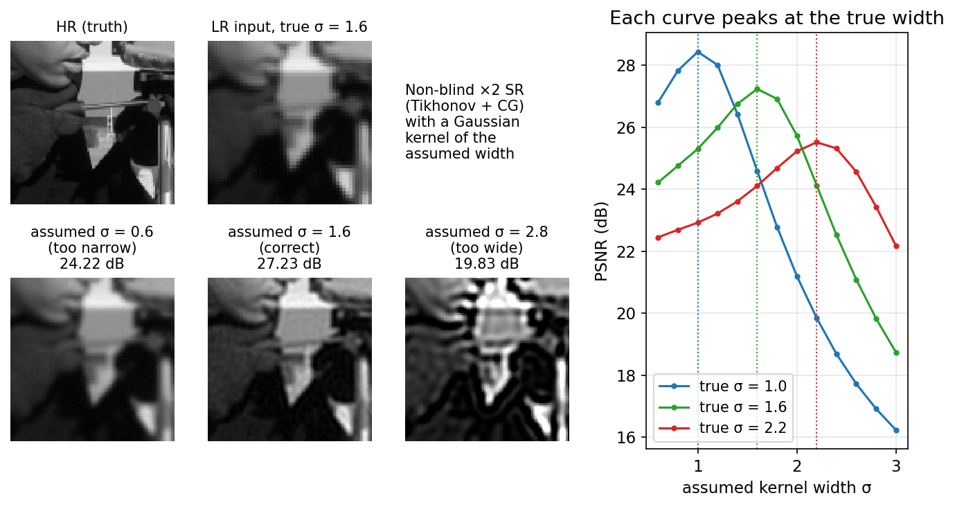
Plain version. Give a non-blind solver the wrong kernel and it does exactly what you asked: it undoes the wrong blur. Too little assumed blur leaves the image soft; too much assumed blur sharpens edges that were already sharp until they ring.
The snippet makes this concrete with the simplest possible non-blind ×2 SR: it solves
with conjugate gradients, where is a Gaussian kernel of the assumed width , was produced with a true width , is the image gradient (implemented through the Laplacian in the normal equations), and weights the smoothness prior.
Code · Python · 39 lines
import numpy as np
from scipy import ndimage as ndi
from scipy.sparse.linalg import LinearOperator, cg
from skimage import data, img_as_float64

s = 2                                                   # scale factor
x = img_as_float64(data.camera())[128:384, 128:384]     # HR test crop (256 x 256)
H, W = x.shape

def blur(z, sigma):                                     # circular Gaussian blur (self-adjoint)
    return ndi.gaussian_filter(z, sigma, mode="wrap")

def A(z, sigma):                                        # degradation: blur, then keep every s-th pixel
    return blur(z, sigma)[::s, ::s]

def At(r, sigma):                                       # its adjoint: zero-fill upsampling, then blur
    up = np.zeros((H, W)); up[::s, ::s] = r
    return blur(up, sigma)

def lap(z):                                             # discrete Laplacian (smoothness prior)
    return ndi.laplace(z, mode="wrap")

def nonblind_sr(y, sigma, lam=2e-3):
    """Solve min_x ||A_sigma x - y||^2 + lam ||grad x||^2 with conjugate gradients."""
    op = LinearOperator((H * W, H * W), dtype=float,
                        matvec=lambda v: (At(A(v.reshape(H, W), sigma), sigma) - lam * lap(v.reshape(H, W))).ravel())
    sol, _ = cg(op, At(y, sigma).ravel(), maxiter=200)
    return sol.reshape(H, W)

def psnr(a, b):
    return 10 * np.log10(1.0 / np.mean((a - np.clip(b, 0, 1)) ** 2))

rng = np.random.default_rng(0)
assumed = [0.6, 1.0, 1.6, 2.2, 2.8]
print("true \\ assumed " + "".join(f"{a:7.1f}" for a in assumed))
for true in [1.0, 1.6, 2.2]:
    y = A(x, true) + 0.003 * rng.standard_normal((H // s, W // s))   # LR observation
    row = [psnr(x, nonblind_sr(y, a)) for a in assumed]
    print(f"sigma = {true:.1f}      " + "".join(f"{p:7.2f}" for p in row))
Output
true \ assumed     0.6    1.0    1.6    2.2    2.8
sigma = 1.0        26.80  28.43  24.59  19.84  16.91
sigma = 1.6        24.22  25.30  27.23  24.13  19.83
sigma = 2.2        22.45  22.92  24.11  25.51  23.43
Every row peaks on the diagonal, where the assumed width equals the true one (our own toy numbers, in dB). The losses are asymmetric: assuming too wide a kernel is punished much harder than assuming too narrow a kernel (for true , assuming 2.8 costs 11.5 dB, assuming 0.6 costs 1.6 dB), because over-deblurring amplifies noise and creates ringing, while under-deblurring only leaves blur. Figure 1 shows the three cases for true . This is the signature IKC learns to read [8].
Degradation representation learning
Plain version. You do not need to know the kernel’s exact shape to fix it; you need to know which kind of damage this image has, well enough to tell it apart from other kinds. So learn a compact “fingerprint” of the damage, without ever being told the true kernel.
DASR (Wang et al.) learns such a fingerprint with contrastive learning [14]. Its assumption is that the degradation is the same everywhere in one image and differs between images. Two patches from the same LR image are therefore a positive pair, and patches from other images are negatives. An encoder maps each patch to a vector, and an InfoNCE loss with a queue of negatives (as in MoCo [33]) pulls positives together and pushes negatives apart; the resulting representation then predicts the weights of depth-wise convolutions and channel-wise scaling factors inside the SR network. KDSR keeps the “implicit representation” idea but trains a teacher that sees the HR–LR pair and distils its representation into a student that sees only the LR image, which lets the representation cover combinations of blur, noise and JPEG for which no explicit label exists [15]. The other DASR, by Liang et al., goes the opposite way: a tiny regression network predicts explicit degradation parameters and uses them to mix several convolutional experts into one efficient SR network [18].
What to remember: a degradation embedding replaces “estimate the kernel, pixel by pixel” with “recognize the kind of degradation”, which avoids explicit kernel labels but still depends on the degradation diversity of the training data and does not guarantee robustness to an unseen family.
Optional: DASR (in the Paper guides). The contrastive loss with every symbol, the degradation-aware convolution, and the ablation that removes each part.
Implicit modelling by degradation synthesis
Plain version. Stop trying to describe one image’s damage. Instead, write a damage generator that is wild enough to produce almost any damage a real photo could have, use it to make millions of training pairs, and train one network on all of them.
BSRGAN: shuffle the steps
BSRGAN argues that blur, downsampling and noise are the key factors, but that real images do not apply them in one fixed order [16]. Its practical degradation model widens each factor (two blurs, one isotropic and one anisotropic Gaussian; several downsamplers including nearest, bilinear, bicubic and a down-up resize; Gaussian noise, JPEG noise and processed camera sensor noise generated with a reverse-forward camera pipeline) and applies them in a randomly shuffled order, followed by a final JPEG compression. The bicubic and classical degradation models become special cases. The same ESRGAN-style network [34] is then trained on these pairs, first with an L1 loss (BSRNet) and then with added perceptual and adversarial losses (BSRGAN).
Real-ESRGAN: repeat the steps
Real-ESRGAN keeps the classical order but applies it twice, a “second-order” degradation, arguing that a real web image was typically degraded by a camera, then by editing, then by one or more rounds of compression and resizing [17]. Each round draws blur (Gaussian, generalized Gaussian, plateau-shaped or sinc kernels), a random resize, Gaussian or Poisson noise and JPEG compression with fresh parameters; a final resize and sinc filter are treated as a pair whose order relative to JPEG is randomly swapped. Its finite sinc kernels approximate an ideal low-pass filter and can produce ringing and overshoot, which real images acquire from sharpening and compression; training on it teaches the network to remove such halos instead of amplifying them. Because the degradation space is so large, Real-ESRGAN also replaces ESRGAN’s discriminator with a U-Net-shaped one [35] that judges every pixel, stabilized with spectral normalization [36].
Optional: The high-order degradation pipeline, step by step and Sinc filters and ringing (in the Supplementary notes). The full sampling procedure, and why an ideal low-pass filter rings.
Optional: BSRGAN and Real-ESRGAN (in the Paper guides). Every step and parameter range, the losses, the test sets and the ablations.
How training pairs are produced
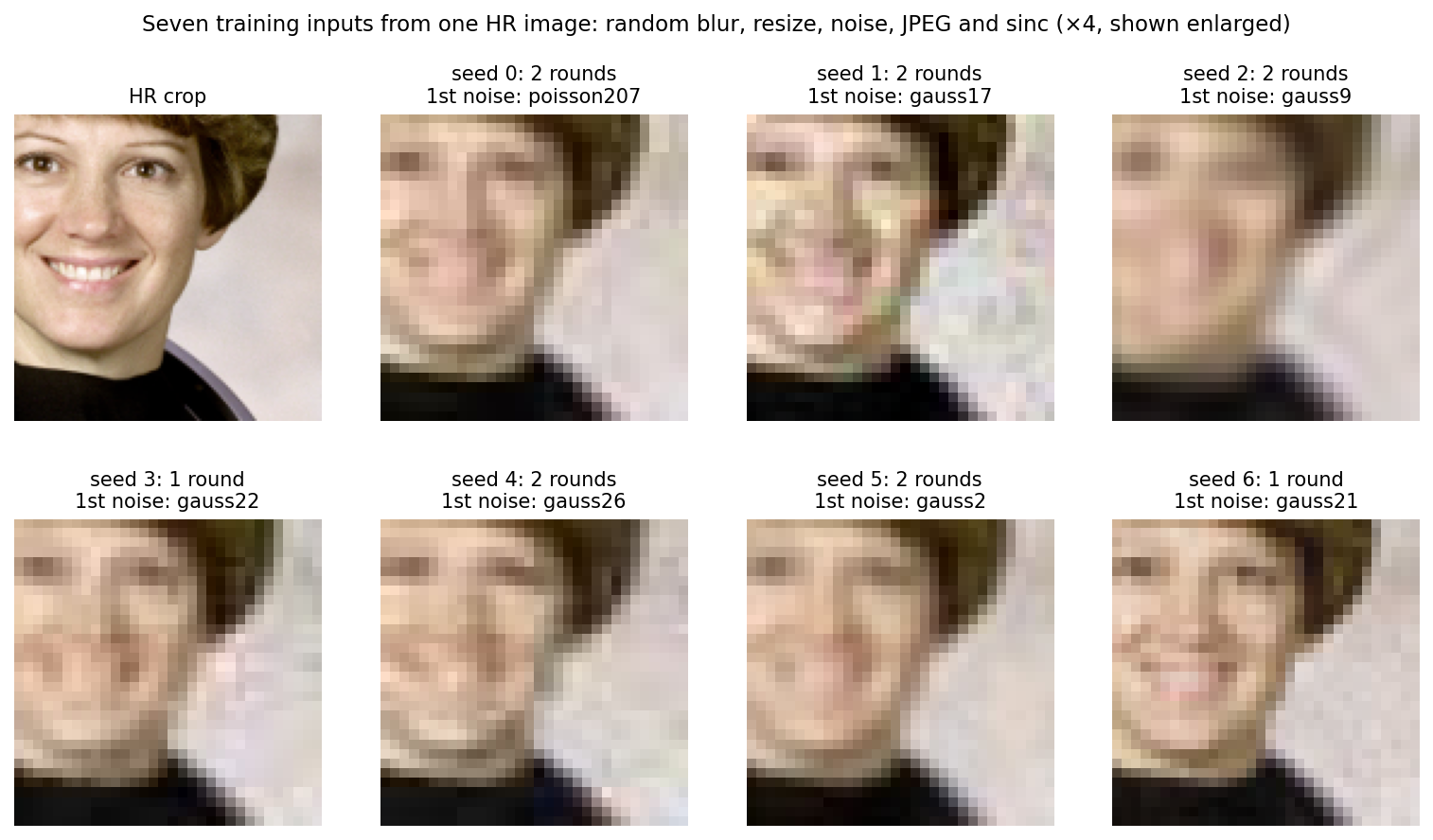
The snippet implements a compact second-order pipeline in the spirit of Real-ESRGAN: two rounds of blur, random resize, noise and JPEG, then swapping JPEG with a final resize-and-sinc pair. The blur sizes, the noise ranges of the first round and the JPEG qualities follow the paper [17]. This teaching version simplifies the resize distribution, shot-noise model and kernel family; it sometimes skips the whole second round, whereas the official pipeline skips only its blur. It is not a reproduction of the training recipe.
Code · Python · 76 lines
import numpy as np, cv2
from scipy import ndimage as ndi
from scipy.special import j1
from skimage import data, img_as_float32

def gaussian_kernel(rng, size, smax):
    """Random isotropic or anisotropic Gaussian: k(c) ~ exp(-0.5 c^T S^-1 c), normalized."""
    s1, s2 = rng.uniform(0.2, smax, 2)
    if rng.random() < 0.5:
        s2 = s1                                                     # isotropic half of the time
    th = rng.uniform(0, np.pi)
    R = np.array([[np.cos(th), -np.sin(th)], [np.sin(th), np.cos(th)]])
    S = R @ np.diag([s1**2, s2**2]) @ R.T
    ax = np.arange(size) - size // 2
    C = np.stack(np.meshgrid(ax, ax, indexing="ij"), -1)
    k = np.exp(-0.5 * np.einsum("...i,ij,...j", C, np.linalg.inv(S), C))
    return k / k.sum(), f"gauss({s1:.1f},{s2:.1f})"

def sinc_kernel(size, wc):
    """2-D sinc low-pass: k(r) = wc J1(wc r) / (2 pi r), with k(0) = wc^2 / (4 pi)."""
    ax = np.arange(size) - size // 2
    r = np.hypot(*np.meshgrid(ax, ax, indexing="ij"))
    with np.errstate(invalid="ignore", divide="ignore"):
        k = np.where(r == 0, wc**2 / (4 * np.pi), wc * j1(wc * r) / (2 * np.pi * r))
    return k / k.sum()

def jpeg(img, q):
    ok, buf = cv2.imencode(".jpg", (np.clip(img, 0, 1) * 255).round().astype(np.uint8)[..., ::-1],
                           [cv2.IMWRITE_JPEG_QUALITY, int(q)])
    return cv2.imdecode(buf, cv2.IMREAD_COLOR)[..., ::-1].astype(np.float32) / 255

def one_round(img, rng, log, smax, nmax):
    """blur -> random resize -> noise -> JPEG: one 'classical' degradation."""
    size = int(rng.choice(np.arange(7, 22, 2)))
    if rng.random() < 0.1:
        k, name = sinc_kernel(size, rng.uniform(np.pi / 3, np.pi)), "sinc"
    else:
        k, name = gaussian_kernel(rng, size, smax)
    img = np.stack([ndi.convolve(img[..., c], k, mode="reflect") for c in range(3)], -1)
    f = rng.uniform(0.3, 1.2)                                       # resize factor (illustrative range)
    interp = rng.choice([cv2.INTER_AREA, cv2.INTER_LINEAR, cv2.INTER_CUBIC])
    img = cv2.resize(img, None, fx=f, fy=f, interpolation=interp)
    if rng.random() < 0.5:                                          # Gaussian noise, sigma in 1..nmax (8-bit units)
        sig = rng.uniform(1, nmax) / 255
        shape = img.shape[:2] + ((1,) if rng.random() < 0.4 else (3,))   # gray or color noise
        img = img + sig * rng.standard_normal(shape); noise = f"gauss{sig * 255:.0f}"
    else:                                                           # shot noise with a random photon count
        peak = 10 ** rng.uniform(1.5, 3)
        img = rng.poisson(np.clip(img, 0, 1) * peak) / peak; noise = f"poisson{peak:.0f}"
    q = rng.uniform(30, 95)
    img = jpeg(img, q)
    log.append(f"{name} x{f:.2f} {noise} q{q:.0f}")
    return img

def degrade(hr, rng, scale=4):
    """Second-order pipeline in the spirit of Real-ESRGAN (parameter ranges partly our own)."""
    log = []
    img = one_round(hr, rng, log, smax=3.0, nmax=30)
    if rng.random() < 0.8:
        img = one_round(img, rng, log, smax=1.5, nmax=25)          # second, milder round
    h, w = hr.shape[0] // scale, hr.shape[1] // scale
    def resize_sinc(z):
        z = cv2.resize(z, (w, h), interpolation=cv2.INTER_AREA)
        k = sinc_kernel(15, rng.uniform(np.pi / 3, np.pi))  # same kernel for all color channels
        return np.stack([ndi.convolve(z[..., c], k, mode="reflect") for c in range(3)], -1)
    final = [lambda z: jpeg(z, rng.uniform(30, 95)), resize_sinc]
    if rng.random() < 0.5:
        final = final[::-1]                                         # swap JPEG with the resize-and-sinc pair
    for op in final:
        img = op(img)
    return np.clip(img, 0, 1), log

hr = img_as_float32(data.astronaut())                               # (512, 512, 3)
for seed in range(3):
    lr, log = degrade(hr, np.random.default_rng(seed))
    print(f"seed {seed}: LR {lr.shape} | " + " ; ".join(log))
Output
seed 0: LR (128, 128, 3) | gauss(0.3,0.2) x0.85 poisson207 q64 ; gauss(0.9,0.9) x0.84 gauss5 q90
seed 1: LR (128, 128, 3) | gauss(0.6,0.6) x1.04 gauss17 q71 ; gauss(1.4,0.6) x0.40 poisson42 q40
seed 2: LR (128, 128, 3) | gauss(2.5,0.5) x0.47 gauss9 q67 ; gauss(0.3,1.1) x1.04 gauss19 q50
Each line is one training input: two rounds with different kernels (gauss(σ1,σ2) lists the two axis widths), resize factors, noise types and JPEG qualities. In training, the HR patch is paired with its LR version and a fresh degradation is drawn every time, so the network repeatedly encounters newly sampled damage. Figure 2 shows seven such inputs from one face; they differ much more than the bicubic inputs of DLCV 09A would. Real-ESRGAN generates its pairs on the GPU and keeps a pool of 180 recent pairs from which batches are drawn, because a batch produced in one call would otherwise share one resize factor [17].
Later refinements
Synthetic degradation is an important data source for the real-world SR methods discussed here. StableSR, SeeSR, SUPIR and ResShift all train on the Real-ESRGAN pipeline [26], [29], [30], [31]. Two lessons came later. Range can matter more than complexity: DiffBIR trains the restoration stage that produces its diffusion model’s conditions on a classical first-order model with wide parameter ranges, and reports better no-reference scores than with the Real-ESRGAN pipeline, which it describes as complex but with smaller ranges [27]. GAN artifacts need their own treatment: LDL computes an artifact map from local residual statistics and uses it to penalize artifact regions during GAN training, improving both fidelity and perceptual quality [37].
Real paired and unpaired data
Plain version. Instead of imitating camera damage, photograph it. Either capture the same scene at two zoom levels to get true LR–HR pairs, or, if pairs are impossible, learn from unpaired collections of real low-quality and high-quality images.
Captured pairs
RealSR photographs each scene with a DSLR at several focal lengths; the long-focal-length shot is the HR image and the short one, after registration and color correction, is the LR image [19]. DRealSR extends the capture to five DSLR cameras for more diverse degradations [20]. City100 collects pairs for both a DSLR and a smartphone by changing the focal length or the shooting distance, to study the trade-off between resolution and field of view [21]. The DPED photos, taken simultaneously with phones and a DSLR, are often used as real low-quality test inputs without ground truth [38]. Captured pairs offer reference images for measuring fidelity on real degradations, but they are small, specific to the cameras used, and slightly misaligned, and a model trained on one camera pair does not cover a phone image from the internet.
Unpaired learning and domain translation
When no pairs exist, GANs can translate between domains. CinCGAN first maps a noisy, blurry real LR image to a clean LR domain with a cycle-consistent GAN, super-resolves it with a pretrained network and then fine-tunes both stages end to end [22]. Bulat et al. go the other way: a High-to-Low GAN learns, from unpaired HR and real LR face images, how to degrade HR images realistically, and its outputs train a Low-to-High network with paired supervision [23]. Lugmayr et al. learn to put natural sensor characteristics back into bicubically downscaled images, again to synthesize realistic pairs [39]; frequency separation (DSGAN and FSSR) applies the adversarial loss only to high frequencies, because downsampling preserves the low ones [24]. Ji et al. estimate real blur kernels and extract real noise patches from the test-domain images and inject both into the classical model, which won the NTIRE 2020 real-world SR challenge [25], [40]. Liu et al. note that this data-distribution family is data-hungry and that GAN-based training often produces severe artifacts and fake textures [3].
Real-world SR with generative priors
Plain version. The networks above learn what photos look like from a few thousand training images. Large text-to-image diffusion models supply priors learned from broad image collections. Since about 2023, several real-world SR methods keep such a model (almost) frozen and add a small network that shows it the LR image, so that it “paints in” detail that fits.
Why a generative prior
When the input is badly damaged, most of the HR detail is simply not in the LR image, and an L2 regression network targets a conditional mean, which can average incompatible details; other losses target different statistics. A generative model instead returns one plausible answer. DLCV 09B explains why this costs PSNR, how diffusion sampling works (diffusion in one page), and why a strong prior can invent content (the hallucination problem). Here we concentrate on what is specific to SR: how each method feeds the LR image to the prior, what extra condition it uses, and what knob it offers between fidelity and realism.
All methods in this section train on synthetic pairs from the Real-ESRGAN pipeline or a similar one, and most build on Stable Diffusion, a latent diffusion model: an autoencoder compresses a image into a latent (a factor of 8 per side), and the denoising network works in that latent space [41]. Many adapt ControlNet, which attaches a trainable copy of the denoiser’s encoder to a frozen model through zero-initialized convolutions [42].
What each method conditions on
| Method | Prior | How the LR image enters | Extra condition | Fidelity knob | Steps (as reported) |
|---|---|---|---|---|---|
| StableSR [26] | Stable Diffusion 2.1, frozen | Time-aware encoder + spatial feature transform (SFT) layers in every residual block | none (null prompt) | Controllable feature wrapping weight in the decoder | 200 (DDPM) |
| DiffBIR [27] | Stable Diffusion 2.1, frozen | First cleaned by a restoration network, then the cleaned image enters an IRControlNet | negative prompt | Region-adaptive restoration guidance scale | 50 |
| PASD [28] | Stable Diffusion | Degradation-removal module and pixel-aware cross-attention | high-level semantic features and captions | Adjustable noise schedule | 20 |
| SeeSR [29] | Stable Diffusion 2, frozen | ControlNet on the LR latent; LR latent also mixed into the starting noise | Degradation-aware tags (hard prompts) and tagger embeddings (soft prompts) | — | 50 |
| SUPIR [30] | SDXL, frozen | Degradation-robust encoder, trimmed ControlNet with ZeroSFT connectors | Captions from a multimodal LLM; negative-quality prompts | Restoration-guided sampling | 100 (EDM) |
| ResShift [31] | Trained from scratch (latent space of a VQGAN) | The chain starts at the LR image and shifts the residual | none | Noise schedule , | 15 |
Step counts are the defaults reported in each paper; the SeeSR supplementary material times them side by side on one V100 GPU for a task: 18.70 s for StableSR (200 steps), 5.85 s for DiffBIR (50), 6.07 s for PASD (20), 7.24 s for SeeSR (50) and 1.12 s for ResShift (15), against 0.09 s for Real-ESRGAN [29].
Three design ideas recur:
- Conditioning strength must vary with the noise level. StableSR adds a time embedding to its condition encoder and finds that the encoder supplies its strongest guidance around a signal-to-noise ratio of about , where image content is formed [26].
- Do not show the prior the raw degradation. DiffBIR observes that a diffusion model conditioned directly on noisy or compressed inputs turns the artifacts into content, so it removes the degradation first with an ordinary restoration network and only then regenerates detail [27]. SUPIR fine-tunes its autoencoder’s encoder to be robust to degradations for the same reason [30].
- Semantics help where pixels are gone. PASD and SeeSR extract text from the LR image and feed it to the prior; SeeSR trains its tagger to give the same tags for degraded and clean images, so that a blurry ship is not “recognized” and then painted as a bird [28], [29]. SUPIR uses a multimodal large language model to caption the input and lets users steer restoration with text [30].
Optional: StableSR, DiffBIR, SeeSR, SUPIR (in the Paper guides). Components, training and verified experiments; ResShift is introduced in the one-step SR chapter.
Diffusion transformers and newer priors
Plain version. The denoiser inside the prior is changing from a U-Net to a transformer, and SR methods follow.
DreamClear builds a restorer on a diffusion transformer (DiT), curates one million synthetic high-quality training images with a generative pipeline, and mixes restoration experts with token-wise degradation priors [43]. DiT4SR feeds the LR latent into the attention of a large DiT as its own stream, so that the LR guidance evolves with the diffusion process instead of being injected once, plus a cross-stream convolution for local detail [44]. The trend is the same as in text-to-image generation: bigger and better priors, with the conditioning moved deeper inside the model.
Fidelity, hallucination and the knob
Plain version. A stronger prior paints more convincingly, and paints more that was not there. Methods therefore use controls between “stay close to the input” and “look real”.
The knobs differ in form but not in purpose: StableSR’s blends encoder features of the LR image into the decoder [26]; DiffBIR’s guidance scale pulls each intermediate estimate toward the cleaned image, more strongly in flat regions [27]; SUPIR’s interpolates each step’s prediction toward the LR latent with a weight that decays during sampling [30]; ResShift’s controls how fast the residual is shifted [31]. These controls change the balance of reference fidelity and generated texture; individual metric curves need not be monotonic. StableSR’s coefficient sweep even improves several scores together for some settings [26]. Two hallucination patterns are specific to SR: semantic errors, where a degraded object is reconstructed as a different object (SeeSR’s examples of a ship turned into a bird or a fish), and texture invention in flat regions, where the random starting noise of a sampler is turned into detail on sky or walls (the reason for SeeSR’s LR-embedding start and for SUPIR’s restoration-guided sampling) [29], [30]. Small text and small faces remain difficult for all of them; StableSR, SeeSR and OSEDiff each name these as limitations [26], [29], [45].
Fewer steps
Plain version. Fifty or two hundred network evaluations per image is too slow for a phone or for video. For SR, the LR image already fixes most of the content, so a diffusion model does not need to start from pure noise, and a few steps, or one, can be enough.
ResShift’s 15-step chain is the bridge: it starts from the LR image instead of noise [31]. Distilled and one-step methods go further: SinSR distils ResShift into a single step [46], and OSEDiff fine-tunes Stable Diffusion with low-rank adapters to map the LR latent to the HR latent in one step, regularized by variational score distillation [45]. These one-step and few-step methods, and how their speed is measured, have their own chapter: DLCV 09A.2.
Evaluation in the blind and real-world setting
Plain version. On real photos there is no ground truth, so you cannot compute an error. You can test on synthetic damage where the truth is known, score real outputs with a model of human judgement, or ask people. Each answer is partial, and rankings can disagree.
Full-reference metrics on synthetic test sets
Blind-SR papers in the explicit family use fixed synthetic protocols so that kernels are known: Gaussian8 (eight isotropic Gaussian kernels per scale, applied before bicubic downsampling, defined in IKC [8]) and DIV2KRK (the 100 DIV2K validation images [47], each with its own random anisotropic, noise-perturbed kernel, defined in KernelGAN [12]). Real-world methods use synthetic test sets made with their own training pipeline, for example 3,000 DIV2K-validation crops degraded with the Real-ESRGAN pipeline in StableSR, SeeSR and OSEDiff [26], [29], [45], or BSRGAN’s DIV2K4D with four degradation types [16]. On these sets PSNR and SSIM [48] measure distortion, and LPIPS [49] and DISTS [50] measure perceptual distance to the reference. A caveat: a test set made with a method’s own training pipeline favors that method.
For captured pairs (RealSR, DRealSR) the same metrics apply, but misalignment between the two zoom levels lowers every method’s PSNR and rewards blur; KernelGAN gives the same reason for not using the NTIRE 2018 blind-SR data [12].
No-reference metrics
Plain version. A no-reference (NR) metric predicts how good an image looks without seeing the original. It is a learned or hand-made model of human opinion, and it can be fooled.
The common NR metrics in real-world SR papers are NIQE (distance of an image’s natural-scene statistics from those of pristine images; lower is better) [51], MUSIQ (a multi-scale transformer trained on human ratings; higher is better) [52], MANIQA (an attention-based model that won an NTIRE 2022 IQA challenge track; higher is better) [53] and CLIPIQA (similarity of the image’s CLIP embedding to the prompts “Good photo.” and “Bad photo.”; higher is better) [54]. Their definitions and validation are in DLCV 09. FID, a distance between feature distributions of a set of outputs and a set of real images, is also reported on paired sets [55].
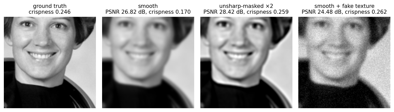
The snippet shows in miniature why such scores must be read with care. It compares a blurry output, an unsharp-masked output and a blurry output with added fine noise, and scores each with PSNR and with a deliberately crude NR “crispness” score, the mean gradient magnitude. Real NR metrics are far better than this, but they share its basic weakness: they score the look of an image, not its correctness.
Code · Python · 25 lines
import numpy as np
from scipy import ndimage as ndi
from skimage import data, img_as_float64
from skimage.color import rgb2gray

hr = img_as_float64(rgb2gray(data.astronaut()))
rng = np.random.default_rng(0)

def psnr(a, b):
    return 10 * np.log10(1.0 / np.mean((a - np.clip(b, 0, 1)) ** 2))

def crispness(img):
    """A crude no-reference score: mean gradient magnitude (higher = 'sharper looking')."""
    return np.mean(np.hypot(ndi.sobel(img, 0), ndi.sobel(img, 1)))

smooth = ndi.gaussian_filter(hr, 1.5)                               # a cautious, blurry restoration
candidates = {
    "smooth (posterior-mean-like)": smooth,
    "unsharp-masked x2": smooth + 2.0 * (smooth - ndi.gaussian_filter(smooth, 2)),
    "smooth + fake fine texture": smooth + 0.04 * rng.standard_normal(hr.shape),
}
for name, img in candidates.items():
    img = np.clip(img, 0, 1)
    print(f"{name:28s} PSNR {psnr(hr, img):6.2f} dB | crispness {crispness(img):.3f}")
print(f"{'ground truth':28s} PSNR    -     | crispness {crispness(hr):.3f}")
Output
smooth (posterior-mean-like) PSNR  26.82 dB | crispness 0.170
unsharp-masked x2            PSNR  28.42 dB | crispness 0.259
smooth + fake fine texture   PSNR  24.48 dB | crispness 0.262
ground truth                 PSNR    -     | crispness 0.246
Both “sharpened” outputs score crisper than the ground truth (our toy numbers), and the one with fake texture is the crispest of all while having the lowest PSNR. PSNR, in turn, prefers the unsharp-masked output only because sharpening partly undid the blur; it would also prefer a slightly blurry correct image to a sharp image with shifted texture. Figure 3 shows the crops.
Why rankings disagree
The published tables show the same tension at full scale:
- NR metrics versus visual quality. On BSRGAN’s 20 real images (RealSRSet), BSRGAN has the worst NIQE of the methods it compares (5.60, against 3.99 to 4.95 for the others), although its authors find its results visually better; they conclude that these NR metrics “do not always match perceptual visual quality” and should be updated for new degradation types [16].
- Fidelity versus realism. In StableSR’s comparison on DIV2K validation crops, StableSR has the best FID, CLIPIQA and MUSIQ but a lower PSNR (23.26 dB) than several GAN methods (up to 24.62 dB) [26]. In SUPIR’s synthetic tests SUPIR leads every NR metric and trails in PSNR, SSIM and LPIPS, and its authors show cases where the metrics prefer a visibly worse result [30].
- NR metrics versus each other. In OSEDiff’s tables, multi-step methods (SeeSR, PASD) score better on NIQE, MUSIQ and MANIQA, while OSEDiff is better on LPIPS, DISTS, FID and CLIPIQA [45]. Which method “wins” depends on the metric chosen.
- Prompts move NR scores. StableSR shows that classifier-free guidance with negative prompts raises CLIPIQA and MUSIQ, and that too strong guidance over-sharpens [26]. A score that a sampling trick can raise is not an independent judge.
Rule of thumb: report at least one full-reference metric on a synthetic or captured set, two NR metrics from different families on real images, and a user study for headline claims; state the test resolution and crop protocol, because methods trained at behave differently on small crops (StableSR reports that SUPIR does poorly on its small crops but better at large resolutions [26]).
User studies and challenges
User studies measure perceived quality or preference, not whether an invented detail belongs to the scene. For example, StableSR collected 1,400 votes from 35 participants on 40 real images [26]; SeeSR measured how often 20 participants confused its output with the ground truth (a confusion rate of 38.6%) and how often they chose it as the best real-world result (57.1%) [29]. Good practice (hidden method names, randomized order, enough images and raters) is described in DLCV 09.
The challenges trace the field’s shift from known to unknown degradations:
- NTIRE 2018 SR had one bicubic track and three tracks with realistic unknown downgrading operators that simulated a camera pipeline, learnable from provided training pairs [56].
- NTIRE 2019 Real Image SR used captured pairs, introducing RealSR (DSLR images at two focal lengths) [57].
- AIM 2019 and NTIRE 2020 Real-World SR provided no pairs at all, only source-domain LR images (and in one track unpaired high-quality targets), and ranked entries by perceptual quality, in 2020 through a human study [58], [40].
- AIM 2020 Real Image SR used captured pairs at ×2, ×3 and ×4 and ranked by PSNR and SSIM [59].
- NTIRE 2025 ×4 SR returned to bicubic inputs but added a perceptual track ranked by a perceptual score next to the PSNR-ranked restoration track [60].
Failure modes
Plain version. Real-world SR fails in two directions: it misreads the damage (and so removes too little or too much), or it trusts its prior too much (and so invents).
- Out-of-distribution degradations. A synthesis-trained model has no guarantee of handling damage outside its training pipeline; Real-ESRGAN lists unknown, out-of-distribution degradations among its limitations and notes that it may even amplify them [17].
- Kernel misestimation. In explicit methods a wrong kernel gives the blur or ringing of Figure 1; spatially varying blur breaks the assumption of a single kernel.
- GAN textures and artifacts. Real-ESRGAN reports twisted lines from aliasing and unpleasant GAN artifacts [17]; BSRGAN reports “bubble” artifacts in texture regions [16]; LDL was designed to suppress such artifacts [37].
- Semantic hallucination. Diffusion-prior methods can reconstruct the wrong object or invent texture in flat regions; degraded small text and faces are the hardest cases [29], [26].
- Color shifts. Diffusion models can shift colors; StableSR corrects them by matching each output channel’s mean and variance to the input, or by replacing the output’s low-frequency wavelet band with the input’s [26].
- Tiling seams and resolution effects. Models trained on crops need tiling for large images; StableSR shows block inconsistency without its aggregation sampling, and performance depends on the test resolution [26].
- Metric gaming. Sharpening, added grain or prompt tricks can raise NR scores without improving fidelity (Figure 3).
A cheap sanity check works for every method: degrade the SR output back to the input size with a plausible model and compare it with the input. Large differences in flat regions or on text mean that the method changed content the input did measure. As DLCV 09B explains, passing this check is a useful diagnostic but not a proof of correctness: the true degradation is itself unknown.
Modern view
Survey papers
Plain version. Two surveys define the vocabulary of this chapter, one for blind SR and one for real-world SR; a diffusion-SR survey and a broad recent SR survey extend them.
- Liu et al., “Blind Image Super-Resolution: A Survey and Beyond” (TPAMI) [3]. Covers: blind SR methods, datasets and earlier challenges, with a comparison on synthetic and real images. Taxonomy: explicit modelling with external data (image-specific adaptation without kernel estimation, such as SRMD, UDVD and USRNet, and with kernel estimation, such as IKC and DAN), explicit modelling with a single image (internal statistics: KernelGAN, ZSSR), and implicit modelling with external data (data-distribution learning with GANs: CinCGAN, FSSR and others). Takeaways: the taxonomy reveals a gap, implicit modelling from a single image; data-distribution methods are data-hungry and produce GAN artifacts; fair comparison is hard because methods assume different degradations.
- Chen et al., “Real-World Single Image Super-Resolution: A Brief Review” (Information Fusion 2022) [4]. Covers: real-world datasets (RealSR, City100, DRealSR and others) and metrics, with comparisons of quality and speed. Taxonomy: degradation-modelling-based (IKC, DAN, KernelGAN), image-pairs-based, domain-translation-based (CinCGAN) and self-learning-based (ZSSR). Takeaway: results on synthetic data overestimate how well methods super-resolve real images.
- Moser et al., “Diffusion Models, Image Super-Resolution, and Everything” (TNNLS 2025) [5]. Covers: diffusion foundations and SR methods by input domain, conditioning, guidance and corruption space. Takeaways: realism has improved greatly; compute, comparability across papers and color shifts remain open.
- Zhang et al., “Deep-Learning-Empowered Super Resolution: A Comprehensive Survey and Future Prospects” (Proceedings of the IEEE 2025) [61]. Covers: single-image, video, stereo and light-field SR, with a taxonomy by backbone (CNN, transformer, GAN, diffusion), datasets, evaluation protocols and complexity. Use: a wide index into the literature, including the real-world and diffusion methods of this chapter.
State of the art, 2023–2026
- Generative priors form an important family of real-world SR methods. StableSR, DiffBIR, PASD, SeeSR and SUPIR attach a frozen text-to-image model through encoders, ControlNet variants and SFT-style connectors [26], [27], [28], [29], [30]; DiT-based restorers such as DreamClear and DiT4SR follow the move of generators to transformers [43], [44].
- Semantics enter as conditions: degradation-aware tags, captions from multimodal models, and text control [29], [30].
- Synthetic pipelines are still the data source: almost every method trains on BSRGAN- or Real-ESRGAN-style degradations, with the training images scaled up (SUPIR reports 20 million images with text; DreamClear one million curated synthetic images) [30], [43].
- Speed is an important engineering objective: from 200 steps to 15 (ResShift) and to one step (SinSR, OSEDiff and later methods; see DLCV 09A.2) [31], [46], [45].
- Explicit blind SR continues in the classical setting with better estimators and representations (DCLS, KDSR), benchmarked on Gaussian8 and DIV2KRK [10], [15].
Open problems
- Faithfulness. No metric reliably separates “sharp and correct” from “sharp and invented”; recent proposals score hallucination directly with multimodal models [62].
- Degradations beyond the pipeline. Spatially varying blur, camera processing, repeated social-media compression and video codecs are only partly covered by synthetic pipelines.
- Evaluation without ground truth. NR metrics disagree with each other and with people, can be raised by sampling tricks, and were not designed for diffusion outputs [16], [26].
- Cost. Large priors (billions of parameters) and multi-step sampling remain far from phone budgets.
- Implicit modelling from a single image, was a gap highlighted by Liu et al.’s survey; it is a useful historical distinction, not evidence that no later method addresses it [3].
Key takeaways
- State what is unknown: degradation parameters, the degradation family or both.
- Classify methods by explicit/implicit degradation handling and external/internal evidence.
- Kernel mismatch can cause blur or ringing; evaluate the estimator and the reconstruction together.
- Synthetic degradation broadens training coverage but cannot guarantee performance on unseen damage.
- Generative priors can supply realistic texture while inventing unsupported detail.
- Combine reference-based tests, several no-reference metric families and user studies; expect different rankings.
Exercises
- The asymmetry of kernel errors. In the kernel-mismatch snippet, (a) set the noise to zero and repeat the table; (b) increase to . How does the penalty for assuming too wide a kernel change in each case, and why?
Hint
Too wide an assumed kernel asks the solver to amplify frequencies that the true kernel did not attenuate, so it boosts noise and creates overshoot. Without noise the loss on the right of each curve shrinks (only ringing remains); a larger damps the amplification and flattens both sides of the curve, at the cost of a lower peak. Print the full rows and compare the drop from the diagonal entry to the entry two steps to the right with the drop two steps to the left.
- Shuffle versus repeat. Modify
degradein the pipeline snippet so that it can also run in a BSRGAN-like mode: build a list of operations (isotropic blur, anisotropic blur, downsampling by 4, noise, JPEG), shuffle it withrng.permutation, apply it, and finish with JPEG. Compare the two modes by the average PSNR of the bicubic upsampling of 50 random LR images against the HR image. Which mode produces harder inputs on average?
Hint
Downsampling placed before blur or noise means the blur acts on LR pixels and the noise is not smoothed by the resize, so shuffled sequences include some very hard cases. Report the mean and the spread over the 50 images; the spread tells you more about the coverage of the degradation space than the mean.
- Reading a no-reference metric. Extend the evaluation snippet with two more candidates: the ground truth with mild JPEG compression (quality 50) and the ground truth shifted by one pixel. Rank all candidates by PSNR and by crispness. Which candidate shows best that PSNR punishes things a viewer would never notice?
Hint
A one-pixel shift can look very similar to the ground truth but has a much lower PSNR; JPEG at quality 50 reduces crispness slightly and adds block edges that may even raise it. This is why captured pairs, which are never perfectly aligned, reward blurrier methods.
- Choosing a method. For each scenario, choose a family from the map and justify it in two sentences: (a) restoring scanned 1990s family photos for a print album; (b) enlarging microscope images for cell counting; (c) a phone’s 2× digital zoom that must run in 30 ms; (d) super-resolving frames from one known security camera model for which you can capture calibration pairs.
Hint
(a) A generative-prior method with a moderate fidelity knob: unknown, mixed damage and a goal of pleasant images. (b) Not a generative prior: counts must not be invented; use a non-blind or captured-pair model with a measured point spread function. (c) Start by measuring a compact synthesis-trained regression or GAN network. Compare a one-step diffusion model only after including its encoder, decoder and memory costs in the target-device budget. (d) Captured pairs for that camera, possibly combined with an explicit kernel measured from calibration targets.
- The KernelGAN ×4 kernel. KernelGAN estimates a ×2 kernel and derives the ×4 kernel as , where is with zeros inserted between its taps. Using two 1-D Gaussians, verify numerically that downscaling by 2 with twice equals downscaling by 4 once with , and find the width of when has width .
Hint
Downscaling twice means . Moving the second convolution in front of the first decimation dilates it by 2. For Gaussians the widths add in quadrature: . Test with a random 1-D signal of length 256 and np.convolve.
References
- N. Efrat, D. Glasner, A. Apartsin, B. Nadler and A. Levin, “Accurate Blur Models vs. Image Priors in Single Image Super-Resolution,” in Proc. IEEE ICCV, 2013, pp. 2832–2839. doi · CVF
- K. Zhang, W. Zuo and L. Zhang, “Learning a Single Convolutional Super-Resolution Network for Multiple Degradations,” CVPR, 2018. paper
- A. Liu, Y. Liu, J. Gu, Y. Qiao, C. Dong, “Blind Image Super-Resolution: A Survey and Beyond,” IEEE TPAMI (early access), 2022. source
- Honggang Chen, Xiaohai He, Linbo Qing, Yuanyuan Wu, Chao Ren, Ray E. Sheriff, Ce Zhu, “Real-world single image super-resolution: A brief review,” Information Fusion, 2022. source
- B. B. Moser, A. S. Shanbhag, F. Raue, S. Frolov, S. Palacio and A. Dengel, “Diffusion Models, Image Super-Resolution, and Everything: A Survey,” IEEE Transactions on Neural Networks and Learning Systems, vol. 36, no. 7, pp. 11793–11813, 2025. doi · arXiv
- Y. Xu, S. R. Tseng, Y. Tseng, H. Kuo, Y. Tsai, “Unified Dynamic Convolutional Network for Super-Resolution with Variational Degradations,” CVPR, 2020. source
- K. Zhang, L. Van Gool, R. Timofte, “Deep Unfolding Network for Image Super-Resolution,” CVPR, 2020. source
- J. Gu, H. Lu, W. Zuo and C. Dong, “Blind Super-Resolution With Iterative Kernel Correction,” CVPR, 2019. paper
- Z. Luo, Y. Huang, S. Li, L. Wang and T. Tan, “Unfolding the Alternating Optimization for Blind Super Resolution,” NeurIPS, 2020. paper
- Z. Luo, H. Huang, L. Yu, Y. Li, H. Fan and S. Liu, “Deep Constrained Least Squares for Blind Image Super-Resolution,” CVPR, 2022. paper
- T. Michaeli, M. Irani, “Nonparametric Blind Super-resolution,” Proceedings of the IEEE International Conference on Computer Vision, 2013. source
- S. Bell-Kligler, A. Shocher and M. Irani, “Blind Super-Resolution Kernel Estimation using an Internal-GAN,” NeurIPS, 2019. paper
- A. Shocher, N. Cohen and M. Irani, “‘Zero-Shot’ Super-Resolution Using Deep Internal Learning,” in Proc. IEEE/CVF CVPR, 2018, pp. 3118–3126. doi · arXiv
- L. Wang, Y. Wang, X. Dong, Q. Xu, J. Yang, W. An and Y. Guo, “Unsupervised Degradation Representation Learning for Blind Super-Resolution,” CVPR, 2021. paper
- B. Xia, Y. Zhang, Y. Wang, Y. Tian, W. Yang, R. Timofte and L. Van Gool, “Knowledge Distillation Based Degradation Estimation for Blind Super-Resolution,” ICLR, 2023. paper
- K. Zhang, J. Liang, L. Van Gool, R. Timofte, “Designing a Practical Degradation Model for Deep Blind Image Super-Resolution,” Proceedings of the IEEE/CVF International Conference on Computer Vision, 2021. source
- X. Wang, L. Xie, C. Dong, Y. Shan, “Real-ESRGAN: Training Real-World Blind Super-Resolution With Pure Synthetic Data,” Proceedings of the IEEE/CVF International Conference on Computer Vision, 2021. source
- J. Liang, H. Zeng, L. Zhang, “Efficient and Degradation-Adaptive Network for Real-World Image Super-Resolution,” ECCV, 2022. source
- J. Cai, H. Zeng, H. Yong, Z. Cao, L. Zhang, “Toward Real-World Single Image Super-Resolution: A New Benchmark and a New Model,” Proceedings of the IEEE/CVF International Conference on Computer Vision, 2019. source
- P. Wei, Z. Xie, H. Lu, Z. Zhan, Q. Ye, W. Zuo, L. Lin, “Component Divide-and-Conquer for Real-World Image Super-Resolution,” ECCV, 2020. source
- C. Chen, Z. Xiong, X. Tian, Z. Zha, F. Wu, “Camera Lens Super-Resolution,” Proceedings of the IEEE/CVF Conference on Computer Vision and Pattern Recognition, 2019. source
- Y. Yuan, S. Liu, J. Zhang, Y. Zhang, C. Dong, L. Lin, “Unsupervised Image Super-Resolution using Cycle-in-Cycle Generative Adversarial Networks,” CVPR Workshops, 2018. source
- A. Bulat, J. Yang, G. Tzimiropoulos, “To learn image super-resolution, use a GAN to learn how to do image degradation first,” ECCV, 2018. source
- M. Fritsche, S. Gu, R. Timofte, “Frequency Separation for Real-World Super-Resolution,” ICCV Workshops, 2019. source
- X. Ji, Y. Cao, Y. Tai, C. Wang, J. Li, F. Huang, “Real-World Super-Resolution via Kernel Estimation and Noise Injection,” Proceedings of the IEEE/CVF Conference on Computer Vision and Pattern Recognition Workshops, 2020. source
- J. Wang, Z. Yue, S. Zhou, K. C. K. Chan, C. C. Loy, “Exploiting Diffusion Prior for Real-World Image Super-Resolution,” IJCV, 2024. source
- X. Lin, J. He, Z. Chen, et al., “DiffBIR: Towards Blind Image Restoration with Generative Diffusion Prior,” ECCV, 2024. source
- T. Yang, R. Wu, P. Ren, X. Xie, L. Zhang, “Pixel-Aware Stable Diffusion for Realistic Image Super-resolution and Personalized Stylization,” ECCV, 2024. source
- R. Wu, T. Yang, L. Sun, Z. Zhang, S. Li, L. Zhang, “SeeSR: Towards Semantics-Aware Real-World Image Super-Resolution,” Proceedings of the IEEE/CVF Conference on Computer Vision and Pattern Recognition, 2024. source · supplementary experiments
- F. Yu, J. Gu, Z. Li, et al., “Scaling Up to Excellence: Practicing Model Scaling for Photo-Realistic Image Restoration In the Wild,” CVPR, 2024. source
- Z. Yue, J. Wang, C. C. Loy, “ResShift: Efficient Diffusion Model for Image Super-resolution by Residual Shifting,” NeurIPS, 2023. source
- X. Wang, K. Yu, C. Dong, C. C. Loy, “Recovering Realistic Texture in Image Super-Resolution by Deep Spatial Feature Transform,” Proceedings of the IEEE Conference on Computer Vision and Pattern Recognition, 2018. source
- K. He, H. Fan, Y. Wu, S. Xie, R. Girshick, “Momentum Contrast for Unsupervised Visual Representation Learning,” CVPR, 2020. source
- X. Wang, K. Yu, S. Wu, J. Gu, Y. Liu, C. Dong, Y. Qiao and C. C. Loy, “ESRGAN: Enhanced Super-Resolution Generative Adversarial Networks,” in Proc. ECCV Workshops, 2018 (Lecture Notes in Computer Science, 2019), pp. 63–79. doi · arXiv
- O. Ronneberger, P. Fischer and T. Brox, “U-Net: Convolutional Networks for Biomedical Image Segmentation,” in Proc. MICCAI, 2015, pp. 234–241. doi · arXiv
- T. Miyato, T. Kataoka, M. Koyama, Y. Yoshida, “Spectral Normalization for Generative Adversarial Networks,” ICLR, 2018. source
- J. Liang, H. Zeng, L. Zhang, “Details or Artifacts: A Locally Discriminative Learning Approach to Realistic Image Super-Resolution,” Proceedings of the IEEE/CVF Conference on Computer Vision and Pattern Recognition, 2022. source
- A. Ignatov, N. Kobyshev, R. Timofte, K. Vanhoey, L. Van Gool, “DSLR-Quality Photos on Mobile Devices with Deep Convolutional Networks,” ICCV, 2017. source
- A. Lugmayr, M. Danelljan, R. Timofte, “Unsupervised Learning for Real-World Super-Resolution,” arXiv preprint, 2019. source
- A. Lugmayr, M. Danelljan, R. Timofte, et al., “NTIRE 2020 Challenge on Real-World Image Super-Resolution: Methods and Results,” CVPR Workshops, 2020. source
- R. Rombach, A. Blattmann, D. Lorenz, P. Esser, B. Ommer, “High-Resolution Image Synthesis with Latent Diffusion Models,” CVPR, 2022. source
- L. Zhang, A. Rao, M. Agrawala, “Adding Conditional Control to Text-to-Image Diffusion Models,” ICCV, 2023. source
- Y. Ai, X. Zhou, H. Huang, X. Han, Z. Chen, Q. You, H. Yang, “DreamClear: High-Capacity Real-World Image Restoration with Privacy-Safe Dataset Curation,” NeurIPS, 2024. source
- Z. Duan, J. Zhang, X. Jin, et al., “DiT4SR: Taming Diffusion Transformer for Real-World Image Super-Resolution,” ICCV, 2025. source
- R. Wu, L. Sun, Z. Ma, L. Zhang, “One-Step Effective Diffusion Network for Real-World Image Super-Resolution,” NeurIPS, 2024. source
- Y. Wang, W. Yang, X. Chen, et al., “SinSR: Diffusion-Based Image Super-Resolution in a Single Step,” CVPR, 2024. source
- E. Agustsson and R. Timofte, “NTIRE 2017 Challenge on Single Image Super-Resolution: Dataset and Study,” in Proc. IEEE CVPR Workshops, 2017, pp. 1122–1131. doi · CVF
- Z. Wang, A. C. Bovik, H. R. Sheikh and E. P. Simoncelli, “Image Quality Assessment: From Error Visibility to Structural Similarity,” IEEE Transactions on Image Processing, vol. 13, no. 4, pp. 600–612, 2004. doi
- R. Zhang, P. Isola, A. A. Efros, E. Shechtman and O. Wang, “The Unreasonable Effectiveness of Deep Features as a Perceptual Metric,” in Proc. IEEE/CVF CVPR, 2018, pp. 586–595. doi · arXiv
- K. Ding, K. Ma, S. Wang, E. P. Simoncelli, “Image Quality Assessment: Unifying Structure and Texture Similarity,” IEEE TPAMI, 2022. source
- A. Mittal, R. Soundararajan and A. C. Bovik, “Making a “Completely Blind” Image Quality Analyzer,” IEEE Signal Processing Letters, vol. 20, no. 3, pp. 209–212, 2013. doi
- J. Ke, Q. Wang, Y. Wang, P. Milanfar, F. Yang, “MUSIQ: Multi-scale Image Quality Transformer,” ICCV, 2021. source
- S. Yang, T. Wu, S. Shi, S. Lao, Y. Gong, M. Cao, J. Wang, Y. Yang, “MANIQA: Multi-dimension Attention Network for No-Reference Image Quality Assessment,” CVPR Workshops, 2022. source
- J. Wang, K. C. K. Chan, C. C. Loy, “Exploring CLIP for Assessing the Look and Feel of Images,” AAAI, 2023. source
- M. Heusel, H. Ramsauer, T. Unterthiner, B. Nessler, S. Hochreiter, “GANs Trained by a Two Time-Scale Update Rule Converge to a Local Nash Equilibrium,” NeurIPS, 2017. source
- R. Timofte, S. Gu, J. Wu, L. Van Gool, “NTIRE 2018 Challenge on Single Image Super-Resolution: Methods and Results,” Proceedings of the IEEE Conference on Computer Vision and Pattern Recognition Workshops, 2018. source
- J. Cai, S. Gu, R. Timofte, L. Zhang, “NTIRE 2019 Challenge on Real Image Super-Resolution: Methods and Results,” Proceedings of the IEEE/CVF Conference on Computer Vision and Pattern Recognition Workshops, 2019. source
- A. Lugmayr, M. Danelljan, R. Timofte, et al., “AIM 2019 Challenge on Real-World Image Super-Resolution: Methods and Results,” ICCV Workshops, 2019. source
- P. Wei, H. Lu, R. Timofte, et al., “AIM 2020 Challenge on Real Image Super-Resolution: Methods and Results,” ECCV Workshops, 2020. source
- Z. Chen, K. Liu, J. Gong, J. Wang, L. Sun, Z. Wu, R. Timofte, Y. Zhang et al., “NTIRE 2025 Challenge on Image Super-Resolution (×4): Methods and Results,” in Proc. IEEE/CVF CVPR Workshops, 2025, pp. 1525–1535. doi · arXiv
- Le Zhang, Ao Li, Qibin Hou, Ce Zhu, Yonina C. Eldar, “Deep-Learning-Empowered Super Resolution: A Comprehensive Survey and Future Prospects,” Proceedings of the IEEE, 2025. source
- W. Ren, R. Goyal, Z. Hu, T. T. Aumentado-Armstrong, I. Mohomed and A. Levinshtein, “Hallucination Score: Towards Mitigating Hallucinations in Generative Image Super-Resolution,” arXiv:2507.14367, 2025. arXiv
- Real-ESRGAN contributors, “Real-ESRGAN model and ×4-plus training configuration,” official source, accessed 2026-11-02. model · configuration
- D. P. Kingma, J. Ba, “Adam: A Method for Stochastic Optimization,” ICLR, 2015. source
- M. Bevilacqua, A. Roumy, C. Guillemot and M.-L. Alberi Morel, “Low-Complexity Single-Image Super-Resolution based on Nonnegative Neighbor Embedding,” in Proc. BMVC, 2012, pp. 135.1–135.10. doi
- R. Zeyde, M. Elad and M. Protter, “On Single Image Scale-Up Using Sparse-Representations,” in Curves and Surfaces, Lecture Notes in Computer Science, Springer, 2012, pp. 711–730. doi
- D. Martin, C. Fowlkes, D. Tal and J. Malik, “A Database of Human Segmented Natural Images and Its Application to Evaluating Segmentation Algorithms and Measuring Ecological Statistics,” in Proc. IEEE ICCV, 2001, vol. 2, pp. 416–423. doi
- J.-B. Huang, A. Singh and N. Ahuja, “Single Image Super-Resolution from Transformed Self-Exemplars,” in Proc. IEEE CVPR, 2015, pp. 5197–5206. doi · CVF
- J. Kim, J. K. Lee and K. M. Lee, “Accurate Image Super-Resolution Using Very Deep Convolutional Networks,” in Proc. IEEE CVPR, 2016, pp. 1646–1654. doi · arXiv
- C. Ledig, L. Theis, F. Huszár, J. Caballero, A. Cunningham, A. Acosta, A. Aitken, A. Tejani, J. Totz, Z. Wang and W. Shi, “Photo-Realistic Single Image Super-Resolution Using a Generative Adversarial Network,” in Proc. IEEE CVPR, 2017, pp. 105–114. doi · arXiv
- R. Timofte, E. Agustsson, L. Van Gool, M.-H. Yang, L. Zhang et al., “NTIRE 2017 Challenge on Single Image Super-Resolution: Methods and Results,” in Proc. IEEE CVPR Workshops, 2017, pp. 1110–1121. doi · CVF
- Y. Matsui, K. Ito, Y. Aramaki, A. Fujimoto, T. Ogawa, T. Yamasaki and K. Aizawa, “Sketch-Based Manga Retrieval Using Manga109 Dataset,” Multimedia Tools and Applications, vol. 76, no. 20, pp. 21811–21838, 2017. doi
- KernelGAN contributors, “Adversarial losses and kernel constraints,” official source, accessed 2026-11-02. loss definitions · alternating updates
- X. Mao, Q. Li, H. Xie, R. Y. K. Lau, Z. Wang, S. P. Smolley, “Least Squares Generative Adversarial Networks,” ICCV, 2017. source
- DASR contributors, “MoCo logits and contrastive cross-entropy implementation,” official DASR source, commit
51524af8021c94a502ee002e135867a1b75dc7d0, accessed 2026-11-02. encoder · loss - Y. Zhang, K. Li, K. Li, L. Wang, B. Zhong and Y. Fu, “Image Super-Resolution Using Very Deep Residual Channel Attention Networks,” in Proc. ECCV, 2018, pp. 294–310. doi · arXiv
- K. Simonyan and A. Zisserman, “Very Deep Convolutional Networks for Large-Scale Image Recognition,” in Proc. ICLR, 2015. arXiv
- Y. Zhang, X. Huang, J. Ma, et al., “Recognize Anything: A Strong Image Tagging Model,” CVPR Workshops, 2024. source
- E. J. Hu, Y. Shen, P. Wallis, Z. Allen-Zhu, Y. Li, S. Wang, L. Wang, W. Chen, “LoRA: Low-Rank Adaptation of Large Language Models,” ICLR, 2022. source
- D. Podell, Z. English, K. Lacey, A. Blattmann, T. Dockhorn, J. Müller, J. Penna, R. Rombach, “SDXL: Improving Latent Diffusion Models for High-Resolution Image Synthesis,” ICLR, 2024. source
- H. Liu, C. Li, Q. Wu, Y. J. Lee, “Visual Instruction Tuning,” NeurIPS, 2023. source
- T. Karras, M. Aittala, T. Aila, S. Laine, “Elucidating the Design Space of Diffusion-Based Generative Models,” NeurIPS, 2022. source
Check your understanding
This tutorial has 5 exercises. Can you solve them without opening the hints?
Go to the exercises ↑Next DLCV 09A.2 · One-Step Diffusion Super-Resolution · 19 min