DLCV 02A · Face Recognition and Metric Learning
Needs: DLCV 02 · Deep Image Classification
Navigate: this page and this track: Navigate: this page and this track
On this page
- What you’ll learn1 min
- The big picture2 min
- Recognition as comparison: the open-set problem3 min
- The face recognition pipeline3 min
- Embeddings on the hypersphere1 min
- Pair-based losses: contrastive and triplet2 min
- Margin-based softmax losses9 min
- Evaluating verification4 min
- Evaluating identification2 min
- Datasets and benchmarks3 min
- Fairness and demographic differentials3 min
- Presentation attacks1 min
- Privacy, consent and the law1 min
- Failure modes and practical advice1 min
- Modern view2 min
- Key takeaways1 min
- Exercises3 min
- Supplementary notes
- Paper guides
- References
- Aligning a face: the least-squares similarity transform
- How large must the scale s be?
- Margin losses side by side: one formula and its edge cases
- Beyond one center per class: sub-centers, quality-aware margins and Partial FC
- Measuring very small error rates
- Before deep learning: eigenfaces and Fisherfaces
Deep Learning for Computer Vision
What you’ll learn
- Distinguish verification, closed-set identification and open-set identification.
- Trace detection, landmark alignment, normalized embeddings and similarity scoring.
- Compare pair-based losses and angular-margin classification losses.
- Choose thresholds and metrics for verification or gallery search.
- Evaluate dataset suitability, demographic differences, privacy and presentation attacks.
The big picture
A classifier picks one of a fixed list of answers. A face recognition system cannot work that way: the people it will meet next year are not in its training set. Instead it learns a way to measure how alike two faces are, and then decides with a threshold.
This idea, metric learning, is much wider than faces. The same recipe (learn an embedding, compare by distance, decide by a threshold) powers person re-identification (DLCV 07), image retrieval, speaker verification and the contrastive self-supervised methods of ML 06. Faces are where the recipe was pushed hardest, because the scale is extreme (millions of identities, error rates of one in a million) and the stakes are high (phone unlocking, border control, police searches).
Face recognition is also a technology with real social costs: errors fall unevenly on different groups, training data was often collected without consent, and some uses are restricted by law. This chapter treats those topics as part of the engineering, factually and with verified sources.
Two surveys frame the field: Wang and Deng’s review of deep face recognition [1] and NIST’s report on demographic effects in commercial algorithms [2]. We return to both in the Modern view.
Related chapters. The softmax, cross-entropy, ROC and calibration basics are in DLCV 02. Re-identification, the triplet loss for people and the CMC metric are in DLCV 07. Contrastive learning and InfoNCE are in ML 06, and image–text embeddings (CLIP) in ML 10. The classical view of nearest-neighbor matching and of open-set rejection is in PR 04 and PR 10.
Recognition as comparison: the open-set problem
Plain version. Verification asks whether two faces belong to the same person; identification searches stored identities. Both can compare people unseen during training.
Verification, identification, closed and open set
Let be a face image and its embedding, produced by a network with parameters . A comparison of two images produces a similarity score
where is the Euclidean norm. People who have stored reference images are enrolled; their stored embeddings (one or several per person) form the gallery, and a new image to be recognized is a probe. A fixed threshold turns a score into a decision.
| Task | Question | Output | Typical use |
|---|---|---|---|
| Verification (1:1) | Is probe the claimed person ? | accept if , else reject | phone unlock, passport gate |
| Closed-set identification (1:N) | Which of the enrolled people is ? | benchmarks; a known, closed group | |
| Open-set identification (1:N) | Is enrolled, and if so, who? | best match if its score , else “not enrolled” | watch lists, photo search |
| Classification (DLCV 02) | Which training class is ? | one of the classes seen in training | not used for faces at test time |
Here is the gallery embedding of person and is the gallery size. Figure 1 draws the three recognition tasks. The important line is the last one: the classes of a face classifier are the training identities, and at test time almost every probe belongs to someone else. NIST’s description of how deployed systems work makes the same point: a face recognition algorithm has no built-in notion of a particular person; it extracts a feature vector from people it has usually never seen and compares two vectors to produce a score [2].
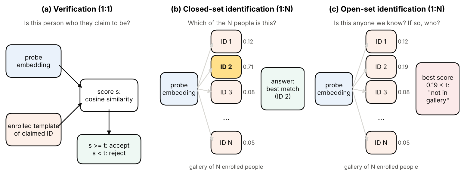
Closed versus open set is a property of the evaluation, not of the network. A closed-set identification test guarantees that every probe has a mate in the gallery, so “pick the best match” is always right in principle. An open-set test includes probes of people who are not enrolled, and then a threshold is unavoidable. Most real searches are open-set. The same distinction appears for generic classifiers as open-set recognition in PR 10; for faces it is the normal case, not an edge case.
Why not just train a classifier?
Plain version. A classifier has outputs only for training identities. Recognition instead reuses its learned embedding to compare new identities.
A standard classifier trained with softmax and cross-entropy on identities already learns a useful penultimate layer. DeepFace [6], one of the first deep systems, trained a network on an identity-labeled dataset of more than 4,000 people and showed that the learned representation generalizes to faces in unconstrained photos; the output layer itself is not used for new people. FaceNet [7] instead trained the embedding directly with a triplet loss. The two lines (classification-style training and pair-based training) then merged into the margin-based softmax losses of 2017–2019 that we study below.
What makes a good embedding for open-set use? Two properties, stated by SphereFace as the ideal criterion: the largest distance within a class should be smaller than the smallest distance between classes [12]. A plain classifier only needs each training sample to fall on the correct side of a decision boundary; it does not care whether the classes are compact. Margins are how we ask for compactness.
The face recognition pipeline
Plain version. Detect the face, locate landmarks, align its crop by rotation and scale, then compute the embedding.
- Detection finds a box around each face.
- Landmark localization finds a few keypoints, usually five: the two eye centers, the nose tip and the two mouth corners.
- Alignment warps the image so that the landmarks match a fixed template, and crops a small, fixed-size image (for example pixels).
- Embedding maps the crop to a vector, usually -normalized to unit length.
- Comparison computes cosine similarities against one template (verification) or a gallery (identification) and applies a threshold.
Detection and landmarks
Face detection is object detection specialized to one class, and the general ideas of DLCV 03 apply. The classical milestone was the Viola–Jones cascade, summarized in DLCV 03’s classical detectors note. Two deep detectors are common front ends in the face-recognition literature, and both predict the five landmarks together with the box:
- MTCNN [4] is a cascade of three convolutional networks that predict face boxes and landmark positions from coarse to fine, trained with an online hard-sample mining strategy.
- RetinaFace [5] is a single-stage detector with multi-task heads; its authors manually annotated five landmarks on the WIDER FACE dataset and showed that this extra supervision helps detect hard faces.
These are not historical details: CosFace aligned its faces with MTCNN landmarks [13], and the ArcFace journal version with RetinaFace landmarks [16]. Detector and landmark errors propagate into everything that follows, so a recognition result is always a result of the whole pipeline.
Alignment by a similarity transform
Plain version. We want every face to look straight at the camera, at the same size and position. A similarity transform (rotate, scale uniformly, shift) is just flexible enough to do this without distorting the face’s shape.
A similarity transform maps a point to
where is the scale, the rotation angle and the translation. It has four parameters , and the equations are linear in them. Given detected landmarks and template positions , we choose the parameters that minimize : ten equations, four unknowns, one least-squares solve. Both CosFace and SphereFace describe their crops as obtained “by similarity transformation” from detected landmarks [12], [13].
Code · Python · 28 lines
import numpy as np

# A toy 5-point template (left eye, right eye, nose tip, left and right mouth
# corners) in a 112 x 112 crop. The coordinates are our own illustration.
template = np.array([[38., 46], [74, 46], [56, 66], [42, 86], [70, 86]])

def fit_similarity(src, dst):
    """Least-squares a, b, tx, ty with dst ~ [[a, -b], [b, a]] @ src + t."""
    n = len(src)
    A = np.zeros((2 * n, 4))
    A[0::2] = np.c_[src[:, 0], -src[:, 1], np.ones(n), np.zeros(n)]
    A[1::2] = np.c_[src[:, 1],  src[:, 0], np.zeros(n), np.ones(n)]
    a, b, tx, ty = np.linalg.lstsq(A, dst.reshape(-1), rcond=None)[0]
    return np.array([[a, -b, tx], [b, a, ty]])

# "Detected" landmarks: the template rotated by 20 degrees, scaled by 1.8,
# shifted into a large photo, plus 1-pixel detector noise.
rng = np.random.default_rng(0)
ang, sc = np.radians(20), 1.8
R = sc * np.array([[np.cos(ang), -np.sin(ang)], [np.sin(ang), np.cos(ang)]])
detected = template @ R.T + [310, 205] + rng.normal(scale=1.0, size=(5, 2))

M = fit_similarity(detected, template)          # photo -> crop
warped = detected @ M[:, :2].T + M[:, 2]
scale = np.hypot(M[0, 0], M[1, 0])
print(f"scale {scale:.3f} (expect {1 / sc:.3f}), "
      f"rotation {np.degrees(np.arctan2(M[1, 0], M[0, 0])):.1f} deg (expect -20.0)")
print(f"RMS landmark error after alignment: {np.sqrt(((warped - template) ** 2).sum(1).mean()):.2f} px")
Output
scale 0.559 (expect 0.556), rotation -19.8 deg (expect -20.0)
RMS landmark error after alignment: 0.56 px
The fit recovers the scale and rotation almost exactly, and the remaining error (0.56 pixels) is what the 1-pixel landmark noise leaves after averaging over five points. The matrix M is then used to warp the whole image into the crop.
Optional: Aligning a face: the least-squares similarity transform (in the Supplementary notes). The normal equations, why a full affine or projective warp is avoided, and the edge cases (reflections, profile faces, wrong landmarks).
The embedding and the template
The embedding network is an ordinary image backbone from DLCV 02 (a ResNet, or a vision transformer) whose last layer outputs a -dimensional vector instead of class scores. FaceNet used [7]; the ArcFace experiments use with crops [16]. When a person is enrolled with several images or a video, the embeddings are combined into one template; ArcFace simply uses the feature center (mean) of all images in the template [16]. Since the network’s output is normalized before comparison, it is natural to renormalize the mean as well.
Embeddings on the hypersphere
Plain version. If we scale every embedding to length 1, all of them live on the surface of a sphere. Then “how alike are two faces” becomes “how small is the angle between their arrows”. Length, which often reflects image quality rather than identity, no longer interferes.
Why normalize, and why cosine
For unit vectors (that is, ),
where is the angle between them. So on the sphere, squared Euclidean distance and cosine similarity are the same ranking, and a threshold on one is a threshold on the other. Normalization removes one degree of freedom that a network can otherwise misuse: with an unnormalized softmax, a network can lower its loss on easy samples simply by making their features longer, without making the classes more compact. NormFace analyzed this and showed that training directly on normalized features needs an extra scale factor to converge [11].
High dimension adds a useful fact: random directions are almost orthogonal. If and are independent and uniformly distributed on the unit sphere in , then and the standard deviation of is . Impostor scores therefore cluster tightly around 0, and the threshold only has to beat the tail of that narrow distribution.
Code · Python · 13 lines
import numpy as np

rng = np.random.default_rng(0)
e = rng.normal(size=(2000, 512))
e /= np.linalg.norm(e, axis=1, keepdims=True)       # 2,000 random unit vectors
a, b = e[0], e[1]
cos = a @ b
print(f"cos = {cos:.4f}   |a-b|^2 = {np.sum((a - b) ** 2):.4f}   2-2cos = {2 - 2 * cos:.4f}")

S = e @ e.T
off = S[np.triu_indices(len(e), 1)]                 # all distinct pairs
print(f"random pairs: mean cos {off.mean():.4f}, std {off.std():.4f}, "
      f"1/sqrt(512) = {1 / np.sqrt(512):.4f}, max {off.max():.3f}")
Output
cos = 0.0472   |a-b|^2 = 1.9057   2-2cos = 1.9057
random pairs: mean cos -0.0000, std 0.0442, 1/sqrt(512) = 0.0442, max 0.214
Among almost two million random pairs in 512 dimensions, the largest cosine is only 0.214. A trained network does not produce random embeddings, but the picture holds: different people sit at angles near , and the job of training is to pull each person’s images into a small cap around one direction.
Pair-based losses: contrastive and triplet
Plain version. The most direct way to train an embedding is to show the network pairs or triples of images and say “these two should be close, those two should be far”. The difficulty is that almost all such examples are already easy, so the network learns little from them unless we search for the hard ones.
Contrastive loss
The contrastive loss, introduced for face verification with a Siamese network by Chopra, Hadsell and LeCun [8] and developed by Hadsell, Chopra and LeCun [9], looks at one pair at a time:
where if the pair shows the same person and otherwise, is a margin, and . Same-person pairs are pulled together; different-person pairs are pushed apart only until they are apart. Up to constant factors and the label convention, this squared-hinge form is the one in [9]; [8] introduced the underlying idea of training a Siamese network so that a learned distance separates same-person from different-person pairs.
Triplet loss and hard-negative mining
The triplet loss of FaceNet [7] compares distances instead of thresholding them. Its definition, and its use in re-identification, are in DLCV 07 and ML 06; in FaceNet’s form, with squared distances on unit-length embeddings,
where is an anchor image, a positive (same person), a negative (another person), the embedding, and the margin. What this chapter adds is the mining question. For an anchor–positive pair with squared distance , a negative at squared distance is
- easy if (zero loss, zero gradient),
- semi-hard if (farther than the positive, but inside the margin; this is FaceNet’s definition [7]),
- hard if (closer than the positive).
FaceNet selected semi-hard negatives online within large mini-batches, because the very hardest negatives early in training led to bad local minima [7]. A later and widely used alternative, batch-hard mining, takes for every anchor in a batch of identities images the farthest positive and the closest negative [10].
Code · Python · 26 lines
import numpy as np

rng = np.random.default_rng(0)
P, Kimg, alpha = 8, 4, 0.2                  # 8 people x 4 images, margin
centres = rng.normal(size=(P, 64))
y = np.repeat(np.arange(P), Kimg)
e = centres[y] + 1.5 * rng.normal(size=(len(y), 64))
e /= np.linalg.norm(e, axis=1, keepdims=True)
d2 = ((e[:, None] - e[None]) ** 2).sum(-1)  # squared distances

easy = semi = hard = 0
for a in range(len(y)):
    for p in np.flatnonzero((y == y[a]) & (np.arange(len(y)) != a)):
        dn = d2[a, y != y[a]]               # distances to all negatives
        hard += (dn < d2[a, p]).sum()
        semi += ((dn >= d2[a, p]) & (dn < d2[a, p] + alpha)).sum()
        easy += (dn >= d2[a, p] + alpha).sum()
tot = easy + semi + hard
print(f"{tot} triplets: easy {easy / tot:.1%}, semi-hard {semi / tot:.1%}, hard {hard / tot:.1%}")

# batch-hard: for each anchor, farthest positive and closest negative
same = y[:, None] == y[None]
hp = np.where(same, d2, -np.inf).max(1)
hn = np.where(~same, d2, np.inf).min(1)
loss = np.maximum(hp - hn + alpha, 0)
print(f"batch-hard loss {loss.mean():.3f}; anchors with non-zero loss: {(loss > 0).sum()} of {len(y)}")
Output
2688 triplets: easy 92.8%, semi-hard 5.4%, hard 1.9%
batch-hard loss 0.213; anchors with non-zero loss: 28 of 32
In this synthetic batch, 92.8% of all 2,688 valid triplets are easy and contribute nothing. Averaging over all triplets would dilute the few useful ones; batch-hard mining finds a non-zero loss for 28 of the 32 anchors. This is the core weakness of pair-based training at face scale: the number of possible triplets grows with the cube of the dataset size, almost all of them are easy, and the result depends on the sampling strategy and the batch composition.
Margin-based softmax losses
Plain version. Instead of comparing images with each other, give every training identity a learned “anchor direction” on the sphere, and train each image to point at its own identity’s direction by a clear margin: not just closer than to the other directions, but closer by a fixed angle. One loss term per image then compares it with all identities at once.
From softmax to normalized softmax
Start from the softmax cross-entropy of DLCV 02. For a feature of image with identity label , a last layer with weight columns and biases gives
Set and write the logit as , where is the angle between and . Now normalize both: , and fixed to a constant . Then the logits are and the prediction depends on angles only [11], [13], [16]:
The scale is necessary because cosines lie in : without it, even a perfect angular arrangement would leave the softmax far from confident, so the loss could not become small. NormFace analyzed this failure to converge [11], and CosFace derived a lower bound for that grows with the number of classes [13]; both CosFace and ArcFace use [13], [16].
Optional: How large must the scale s be? (in the Supplementary notes). CosFace’s lower bound with every symbol defined, a worked example, and what goes wrong when is too small or too large.
Each column is now a unit vector: a class center, or proxy, for identity on the sphere. This is the key structural change compared with pair-based losses. Every image is compared with all class centers in every step, so there is nothing to mine, and the comparison is global rather than limited to one batch. The class centers exist only for training; at test time the last layer is discarded and only the embedding network is kept [16].
Three ways to add a margin
The normalized softmax is satisfied when for all : the feature is closer in angle to its own center than to any other. That puts the decision boundary exactly halfway between two centers, so samples near the boundary are correct but barely. A margin makes the target logit harder to achieve by modifying it from to with , while the other logits stay :
The three classic losses differ only in :
| Loss | Target logit | Margin type | Value in the paper |
|---|---|---|---|
| SphereFace (A-Softmax) [12] | , extended to stay monotone (below) | multiplicative angular | |
| CosFace (LMCL) [13]; also AM-Softmax [14] | additive cosine | , | |
| ArcFace [15], [16] | additive angular | , |
Here is the margin (an integer for SphereFace, a cosine offset for CosFace and an angle in radians for ArcFace), and is the angle to the sample’s own class center; the last column gives the values reported in the papers. Because is not monotone on , SphereFace uses for , [12]. The original SphereFace normalized only the weights and needed help from an ordinary softmax early in training [16]. AM-Softmax [14], published at about the same time as CosFace, uses the same additive cosine margin.
Code · Python · 12 lines
import numpy as np

def sphereface_psi(theta, m=4):
    """SphereFace's monotone extension of cos(m*theta) to [0, pi]."""
    k = np.floor(theta * m / np.pi)
    return (-1) ** k * np.cos(m * theta) - 2 * k

print(" angle  softmax  SphereFace  CosFace  ArcFace")
for deg in [10, 30, 45, 60, 90]:
    t = np.radians(deg)
    print(f"{deg:5d}   {np.cos(t):6.3f}   {sphereface_psi(t):8.3f}   "
          f"{np.cos(t) - 0.35:6.3f}   {np.cos(t + 0.5):6.3f}")
Output
 angle  softmax  SphereFace  CosFace  ArcFace
   10    0.985      0.766    0.635    0.781
   30    0.866     -0.500    0.516    0.520
   45    0.707     -1.000    0.357    0.282
   60    0.500     -1.500    0.150    0.024
   90    0.000     -3.000   -0.350   -0.479
The table shows the target logit (divided by ) at five angles. Every margin lowers the logit of the correct class, so the loss stays large until the angle is small. The penalties grow differently: CosFace subtracts the same 0.35 at every angle; ArcFace’s penalty is small near (0.204 at ) and larger at wide angles; SphereFace with is very strict at wide angles.
The geometry on the circle
Plain version. Picture two class centers on a circle. Without a margin, the circle is split exactly halfway between them. With a margin, each class claims less than half, and a strip in between belongs to nobody: a sample there still has a loss. Training pushes samples out of that strip, toward their own center.
For two classes with centers an angle apart, and a feature on the arc between them, a sample of class 1 is “satisfied” when with . Solving gives the class-1 boundary:
- normalized softmax: (no gap);
- SphereFace: , so ; the gap between the two classes’ boundaries is , which grows with ;
- CosFace: ; the gap is a fixed amount in cosine, so its size in angle depends on ;
- ArcFace: , so ; the gap is exactly radians for every .
ArcFace’s authors call this a margin equal to the geodesic distance on the hypersphere, which is where the name comes from [15], [16]. Figure 2 draws all four cases for ; SphereFace is shown with so that its zone fits on the same picture.
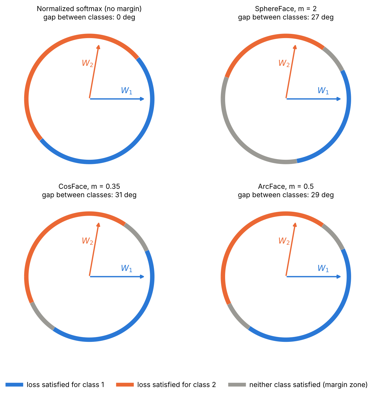
One practical detail follows from the formula: decreases only while . For a sample whose angle to its own center is larger than (a badly misclassified or mislabeled sample), the ArcFace target logit would start to increase again as the sample moves away. An implementation has to handle this range explicitly, for example by switching to a monotone penalty there. In our toy code below, all angles stay well below that range.
Optional: Margin losses side by side: one formula and its edge cases (in the Supplementary notes). The combined margin , the derivation of each boundary, the gradient of the ArcFace logit, and why easy samples stop contributing.
A toy experiment: softmax versus ArcFace
Plain version. We train the same small network on synthetic “faces” twice: once with the ordinary softmax and once with ArcFace. Then we look at how tight the training clusters are and, more importantly, how well the network separates people it never saw.
The data mimic the face problem. Each synthetic identity is a random point in a 4-dimensional “identity” subspace of a 16-dimensional input; every image adds a large random “nuisance” component (standing in for pose and lighting) in the other 12 dimensions and small noise everywhere. The network is one hidden layer of 64 ReLU units followed by a linear map to a embedding. We implement the forward pass and the gradients by hand, including the chain rule through the normalization and through , and use plain gradient descent. We train on 100 identities and test verification on 50 identities that never appear in training. TAR at FAR = 1% (defined in the next section) is the fraction of same-person test pairs accepted when the threshold lets through 1% of different-person pairs.
Code · Python · 61 lines
import numpy as np

rng = np.random.default_rng(0)
D, K = 16, 4                                      # input dim, identity dims
U = np.linalg.qr(rng.normal(size=(D, D)))[0]      # random orthonormal basis

def sample(ids, n_per):
    """Identity signal in 4 directions, large 'pose/light' nuisance in 12."""
    y = np.repeat(np.arange(len(ids)), n_per)
    nuis = 1.5 * rng.normal(size=(len(y), D - K))
    x = ids[y] @ U[:, :K].T + nuis @ U[:, K:].T + 0.3 * rng.normal(size=(len(y), D))
    return x, y

unit = lambda v, ax: v / np.linalg.norm(v, axis=ax, keepdims=True)

def train(x, y, C, d=4, margin=None, s=16.0, steps=800, lr=0.2, H=64):
    """One-hidden-layer embedding net + class centres W, plain gradient descent.
    margin=None: ordinary softmax on raw features; otherwise ArcFace logits."""
    r = np.random.default_rng(1)
    W1 = r.normal(size=(D, H)) / 4; b1 = np.zeros(H)
    W2 = r.normal(size=(H, d)) / 8; W = r.normal(size=(d, C))
    Y = np.eye(C)[y]
    for _ in range(steps):
        h = np.maximum(x @ W1 + b1, 0); z = h @ W2          # embeddings
        if margin is None:
            L = z @ W
        else:
            f, w = unit(z, 1), unit(W, 0)
            th = np.arccos(np.clip(f @ w, -1 + 1e-7, 1 - 1e-7))   # angles to centres
            L = s * np.where(Y > 0, np.cos(th + margin), np.cos(th))
        p = np.exp(L - L.max(1, keepdims=True)); p /= p.sum(1, keepdims=True)
        g = (p - Y) / len(y)                                  # dLoss/dlogits
        if margin is None:
            gz, gW = g @ W.T, z.T @ g
        else:                                                 # chain rule through cos(theta+m)
            gc = g * s * np.where(Y > 0, np.sin(th + margin) / np.sin(th), 1.0)
            gf, gw = gc @ w.T, f.T @ gc
            gz = (gf - (gf * f).sum(1, keepdims=True) * f) / np.linalg.norm(z, axis=1, keepdims=True)
            gW = (gw - (gw * w).sum(0, keepdims=True) * w) / np.linalg.norm(W, axis=0, keepdims=True)
        gh = (gz @ W2.T) * (h > 0)
        W1 -= lr * x.T @ gh; b1 -= lr * gh.sum(0); W2 -= lr * h.T @ gz; W -= lr * gW
    return lambda xx: unit(np.maximum(xx @ W1 + b1, 0) @ W2, 1)

def intra_angle(e, y):            # mean angle (degrees) to own class mean direction
    cen = unit(np.stack([e[y == j].mean(0) for j in np.unique(y)]), 1)
    return np.degrees(np.arccos(np.clip((e * cen[y]).sum(1), -1, 1))).mean()

def tar_at_far(e, y, far=0.01):   # verification on all pairs of unseen people
    i, j = np.triu_indices(len(y), 1)
    sc, same = (e[i] * e[j]).sum(1), y[i] == y[j]
    thr = np.quantile(sc[~same], 1 - far)
    return (sc[same] > thr).mean()

ids = rng.normal(size=(150, K))
xtr, ytr = sample(ids[:100], 10)          # 100 training identities
xte, yte = sample(ids[100:], 10)          # 50 identities never seen in training
for name, m in [("softmax", None), ("norm-softmax", 0.0), ("ArcFace m=0.5", 0.5)]:
    emb = train(xtr, ytr, 100, margin=m)
    print(f"{name:14s} train intra {intra_angle(emb(xtr), ytr):5.1f} deg | "
          f"unseen intra {intra_angle(emb(xte), yte):5.1f} deg | "
          f"unseen TAR@FAR=1% {tar_at_far(emb(xte), yte):.3f}")
Output
softmax        train intra  27.1 deg | unseen intra  43.9 deg | unseen TAR@FAR=1% 0.082
norm-softmax   train intra  16.1 deg | unseen intra  30.1 deg | unseen TAR@FAR=1% 0.098
ArcFace m=0.5  train intra  11.6 deg | unseen intra  24.4 deg | unseen TAR@FAR=1% 0.248
The script runs in about ten seconds on a CPU. In this toy run the mean angle of a training image to its class center drops from 27.1° (softmax) to 16.1° (normalization alone) to 11.6° (ArcFace), and the clusters of unseen people tighten too (43.9° to 24.4°). The verification rate on unseen people at FAR = 1% roughly triples, from 0.082 to 0.248. Two cautions. First, the absolute numbers are low because a 4-dimensional embedding of noisy data is a hard problem; only the comparison matters. Second, these are single runs; with two other random seeds the ordering softmax < normalized softmax < ArcFace stayed the same in our runs, but the exact values changed.
Figure 3 shows the same effect in a 2-D embedding with six identities, where it can be seen directly: softmax spreads each class along a ray (it can lower its loss by lengthening features), while ArcFace packs each class into a short arc.
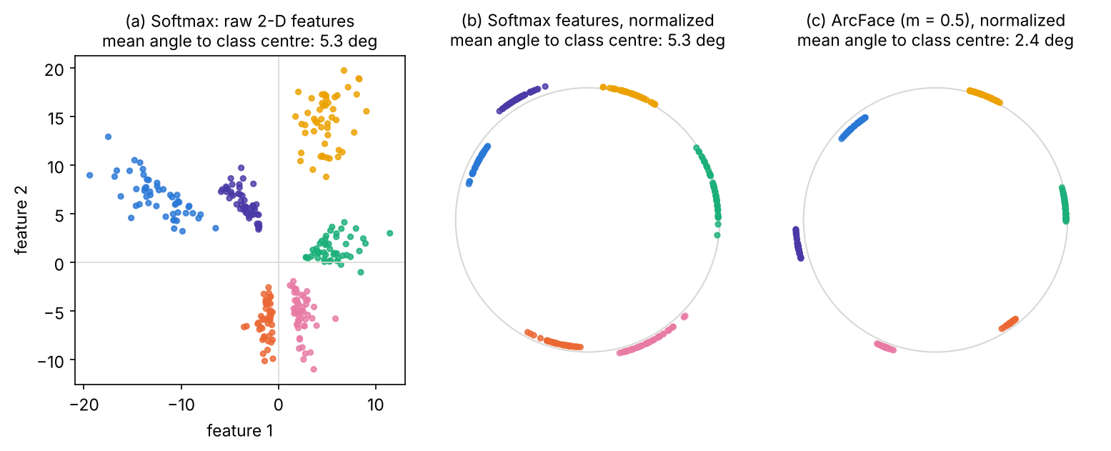
Margins tighten clusters of the training identities directly. Whether that transfers to new people depends on how many and how varied the training identities are; with very few training identities, a network can separate them perfectly and still learn nothing general. That is one reason why face recognition training sets contain hundreds of thousands to millions of identities (see the datasets section).
Class centers, sub-centers and adaptive margins
Plain version. Once each identity has a center, several refinements follow naturally. They all keep the margin softmax and change one thing about the centers or the margin.
Center loss [17], which predates the angular losses, pulls each feature toward a learned center of its class. Sub-center ArcFace [18], [16] gives each identity several centers, so that noisy or mislabeled images can gather away from the clean ones. MagFace [19] and AdaFace [20] tie the margin to image quality, using the feature magnitude, so that very poor images do not dominate training. Partial FC [21] cuts the cost of millions of centers by updating only a sampled subset of them in each step. The one thing to remember: the class centers are a training device, and these methods tune how strictly and how cheaply images are pulled toward them.
Optional: Beyond one center per class: sub-centers, quality-aware margins and Partial FC (in the Supplementary notes). How each variant changes the loss, the problem it targets, and what to watch for when you use it.
Evaluating verification
Plain version. Compare many pairs of photos of the same person (genuine pairs) and many pairs of different people (impostor pairs). A good system gives genuine pairs high scores and impostor pairs low scores. Any threshold then trades two errors: letting impostors in, and turning genuine users away.
Genuine and impostor scores, FAR and TAR
For a threshold on the similarity score ,
FAR is the false accept rate, FRR the false reject rate and TAR the true accept rate. NIST’s evaluations use the equivalent names false match rate (FMR) and false non-match rate (FNMR) for one-to-one comparisons [2], [3]. These are exactly the false-positive rate and the false-negative rate of DLCV 02; the “positive” class is “same person”.
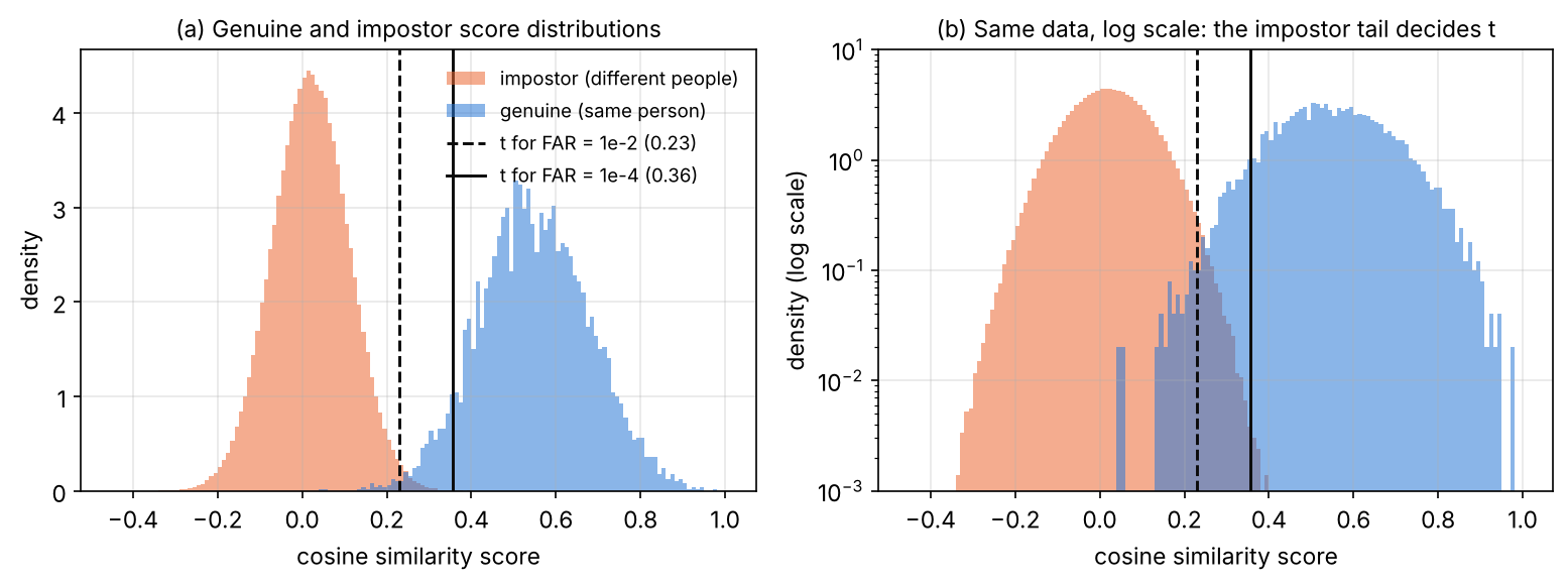
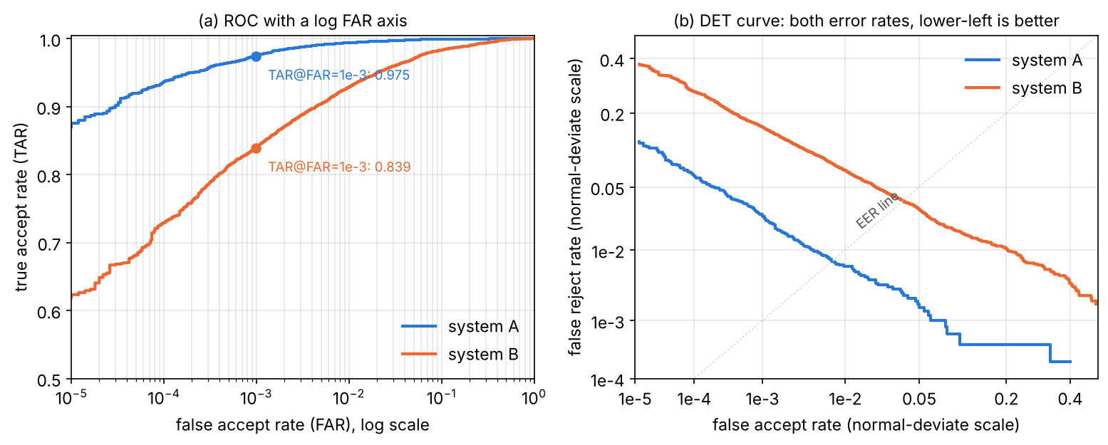
The two distributions are very unequal in size. With people and images each, there are genuine pairs but about impostor pairs, which grows with the square of . Because impostor pairs are so many, operating points are stated as TAR at a fixed FAR: “TAR@FAR = ” is the fraction of genuine pairs accepted when the threshold is set so that one impostor pair in ten thousand is accepted. Benchmarks such as IJB-B and IJB-C report TAR@FAR = [16], and NIST’s ongoing one-to-one evaluation ranks algorithms by FNMR at FMR = on one of its datasets [3].
Code · Python · 15 lines
import numpy as np
from sklearn.metrics import roc_curve

rng = np.random.default_rng(0)
genuine = np.clip(rng.normal(0.55, 0.13, 5_000), -1, 1)       # same-person cosines
impostor = np.clip(rng.normal(0.02, 0.09, 500_000), -1, 1)    # different-person cosines
y = np.r_[np.ones(genuine.size), np.zeros(impostor.size)]
fpr, tpr, thr = roc_curve(y, np.r_[genuine, impostor])

for far in [1e-2, 1e-3, 1e-4]:
    i = np.searchsorted(fpr, far, side="right") - 1          # last point with FPR <= far
    print(f"FAR <= {far:.0e}: threshold {thr[i]:.3f}, TAR {tpr[i]:.3f}, "
          f"false accepts {int(round(fpr[i] * impostor.size))}")
i = np.argmin(np.abs(fpr - (1 - tpr)))
print(f"EER ~ {(fpr[i] + 1 - tpr[i]) / 2:.4f} at threshold {thr[i]:.3f}")
Output
FAR <= 1e-02: threshold 0.231, TAR 0.994, false accepts 4825
FAR <= 1e-03: threshold 0.300, TAR 0.975, false accepts 495
FAR <= 1e-04: threshold 0.356, TAR 0.936, false accepts 49
EER ~ 0.0072 at threshold 0.241
The equal error rate (EER) is the error at the threshold where FAR equals FRR; it is a convenient single number but describes an operating point that a secure system rarely uses. Notice how the threshold moves: lowering FAR from to raises the threshold from 0.231 to 0.356 and costs 5.8 points of TAR. Notice also how few errors the last line is based on: 49 false accepts. A FAR of cannot be measured at all with 500,000 impostor pairs; you need millions of them, and they must be reasonably independent.
Optional: Measuring very small error rates (in the Supplementary notes). The “rule of three”, binomial confidence intervals, and why impostor pairs built from the same images are not independent.
ROC and DET curves
The ROC curve of DLCV 02 plots TAR against FAR. For face verification a logarithmic FAR axis is often useful: operating regions such as FAR between and would be squeezed into the left edge on a linear axis. The axis scale is a presentation choice, not part of the definition of ROC; zero FAR cannot be plotted on a logarithmic axis. The detection error trade-off (DET) curve [22] plots both error rates, FRR against FAR, with both axes transformed by the inverse of the standard normal cumulative distribution function (the “normal deviate” scale). If genuine and impostor scores are both Gaussian, the DET curve is a straight line, and lower-left is better. Martin et al. introduced it for speaker recognition and explained why it tends to be close to linear [22]; it is now standard for biometric systems.
Choosing the threshold
The threshold is part of the system, not of the network, and it must be chosen on data that represent deployment. Three rules follow from the formulas above. (1) Fix the FAR you can tolerate from the application (a phone unlock and a forensic search have very different costs), then choose as the corresponding quantile of impostor scores on a held-out set; tuning on the test set inflates results. (2) Report TAR and FAR together at that threshold, never one alone. (3) Check that the impostor scores of your deployment look like those of your calibration set: a new camera, a new population or a new image quality changes the impostor distribution and therefore the real FAR at a fixed . We return to the last point in the fairness section.
Evaluating identification
Plain version. In a search, the probe is compared with every enrolled person. In a closed-set test we ask: was the right person ranked first (or in the top )? In an open-set test we also ask: when the person is not enrolled at all, did the system stay silent?
Closed set: rank-1 and the CMC curve
For closed-set identification, sort the gallery by similarity to the probe. Rank-1 accuracy is the fraction of probes whose mate is ranked first, and the cumulative match characteristic CMC() is the fraction whose mate is within the top . The formula and code are in DLCV 07; a face gallery usually holds one template per person, so mAP is rarely used.
The crucial effect is gallery size. Each extra enrolled person is one more chance for an impostor to outscore the true mate. MegaFace was built to measure this: it added up to one million distractor photos to the gallery and reported identification and verification as the number of distractors grew from 10 to 1M [24].
Open set: FNIR and FPIR
In an open-set search, the system returns a candidate only if its score reaches a threshold . Two error rates describe it [2]:
A mated search is one whose probe person is enrolled; a non-mated search is one whose probe person is not. FNIR (false negative identification rate) and FPIR (false positive identification rate) play the roles of FRR and FAR for one-to-many search; in this simple version a candidate is returned only at rank 1. If every one of the gallery comparisons of a non-mated probe were an independent trial with false match rate FMR(), then
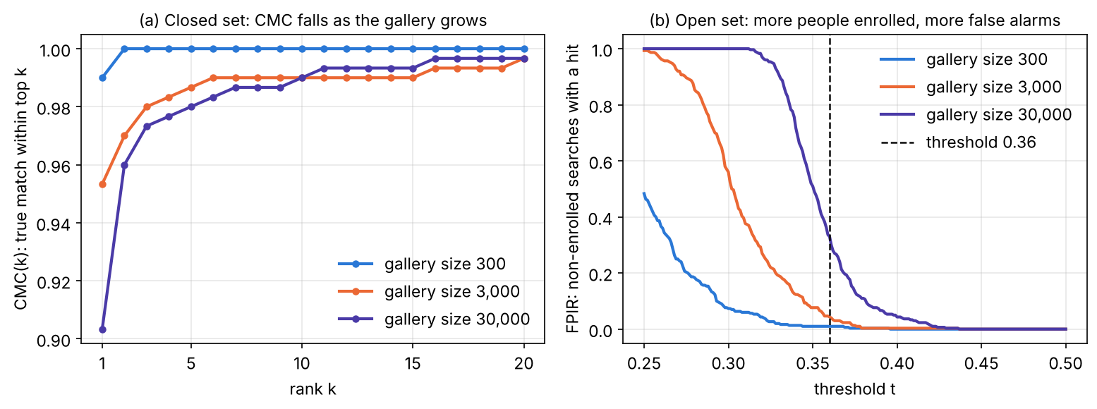
so at a fixed threshold FPIR grows roughly in proportion to the gallery size. This is why one-to-many search needs far lower one-to-one false match rates than verification.
Code · Python · 22 lines
import numpy as np

rng = np.random.default_rng(0)
dim, noise = 128, 1.1
unit = lambda v: v / np.linalg.norm(v, axis=-1, keepdims=True)

def identify(n_gallery, n_probe=300, thr=0.36):
    people = rng.normal(size=(n_gallery + n_probe, dim))
    gallery = unit(people[:n_gallery] + noise * rng.normal(size=(n_gallery, dim)))
    mated = rng.choice(n_gallery, n_probe, replace=False)             # enrolled people
    p_in = unit(people[mated] + noise * rng.normal(size=(n_probe, dim)))
    p_out = unit(people[n_gallery:] + noise * rng.normal(size=(n_probe, dim)))  # not enrolled
    S_in, S_out = p_in @ gallery.T, p_out @ gallery.T
    rank1 = (S_in.argmax(1) == mated).mean()
    # open set: a search "returns" the top candidate only if its score >= thr
    fnir = 1 - ((S_in.argmax(1) == mated) & (S_in.max(1) >= thr)).mean()
    fpir = (S_out.max(1) >= thr).mean()
    return rank1, fnir, fpir

for n in [300, 3_000, 30_000]:
    r1, fnir, fpir = identify(n)
    print(f"gallery {n:6d}: rank-1 {r1:.3f} | threshold 0.36: FNIR {fnir:.3f}, FPIR {fpir:.3f}")
Output
gallery    300: rank-1 0.990 | threshold 0.36: FNIR 0.090, FPIR 0.010
gallery   3000: rank-1 0.953 | threshold 0.36: FNIR 0.113, FPIR 0.043
gallery  30000: rank-1 0.903 | threshold 0.36: FNIR 0.117, FPIR 0.330
With the same synthetic embedding quality, growing the gallery from 300 to 30,000 people lowers rank-1 from 0.990 to 0.903, and at a fixed threshold the share of non-enrolled probes that trigger a false hit rises from 1% to 33%. Figure 6 shows the CMC curves and the FPIR-versus-threshold curves of a similar run. An identification result is meaningless without the gallery size, and an open-set system must be re-thresholded when the gallery grows.
Datasets and benchmarks
Plain version. Training sets for faces are huge lists of web photos grouped by person; test sets define pairs or searches with a fixed protocol. Several of the best-known sets were collected from the web without the consent of the people in them, and some have been withdrawn.
| Dataset | Role | What it contains (as described by its source) | Status |
|---|---|---|---|
| LFW [23] | verification test | unconstrained news photos; about 13K photos of 5K people [24] | saturated; a disclaimer added in 2019 warns against concluding commercial suitability from it [30] |
| IJB-B [27] | verification, identification, clustering | 1,845 subjects; 21,798 still images and 55,026 frames from 7,011 videos, with human-labeled boxes and eye/nose locations | standard test set; media under a Creative Commons license [27] |
| IJB-C [28] | as IJB-B, larger | 3,531 subjects; 31.3K still images and 117.5K frames from 11,779 videos [16] | standard test set [16] |
| MegaFace [24], [25] | identification at scale | 1M distractor photos of more than 690K individuals; a later training set of 4.7M photos of 672,057 identities | decommissioned; data no longer distributed [25] |
| MS-Celeb-1M [26] | training | web images for a benchmark of recognizing one million celebrities linked to a knowledge base | taken down in April 2019 [30] |
| WebFace260M / WebFace42M [29] | training | 4M identities / 260M faces (noisy) and a cleaned 2M identities / 42M faces | described by its authors as the largest public training set [29] |
| DigiFace-1M [31] | training | synthetic faces rendered with a computer-graphics pipeline | synthetic, not photographs of real people |
LFW (Labeled Faces in the Wild) [23] defined unconstrained face verification and its standard protocols. Its accuracy is now saturated: state-of-the-art models exceed 99.8% on it [31], so it no longer separates good systems from very good ones. IJB-B and IJB-C (IARPA Janus Benchmarks) [27], [28] replaced it as the standard academic test: they include video frames, large pose variation and protocols at operationally relevant points such as TAR@FAR = , and they evaluate templates (sets of images) rather than single images. MegaFace [24] made gallery size the central question. NIST’s evaluations [2], [3] use large operational datasets that are not public and test submitted algorithms directly, so they are the reference for deployment-scale error rates.
Withdrawn datasets. MS-Celeb-1M was taken down by Microsoft in April 2019; Peng, Mathur and Narayanan note that the removal followed critical reports, that many of the “celebrities” were fairly ordinary people, that the images had been aggregated without consent, and that Microsoft gave as its reason that the research challenge was over [30]. MegaFace’s own site states that the challenge has concluded and that the data are no longer distributed [25]. The same study found that retracted data often keep circulating through copies, cleaned derivatives and pretrained models, and that licenses did little to restrict such use [30]; the DukeMTMC case in DLCV 07 is similar. In practice: do not use withdrawn datasets or their derivatives, record the provenance and license of every training set, and expect reviewers to ask.
Synthetic training data is one response. DigiFace-1M renders faces with a computer-graphics pipeline and motivates this with bias, label noise and the lack of consent in web-crawled data [31]; DCFace generates identities and styles with a diffusion model [32]. Boutros et al. survey this direction and its open challenges [33].
Fairness and demographic differentials
Plain version. A system can have the same overall accuracy as another and still make many more errors for some groups of people than for others. Because a deployed system usually uses one threshold for everybody, small differences in score distributions between groups can turn into large differences in error rates.
What the measurements show
The most extensive public measurement is NIST’s 2019 report on demographic effects [2]. It processed 18.27 million images of 8.49 million people from four U.S. government datasets through 189 mostly commercial algorithms from 99 developers. Its main findings, in the report’s own framing:
- False positives differed far more than false negatives: across demographic groups, false positive rates often varied by factors of 10 to beyond 100, while false negatives were more algorithm-specific and often varied by factors below 3.
- The pattern depended on the algorithm and the data. For example, with high-quality application photos the highest false positive rates were in West and East African and East Asian people for many algorithms, but with a number of algorithms developed in China the East Asian effect was reversed. False positives were also higher for women than for men and elevated for the elderly and children.
- Image quality mattered for false negatives: results differed between well-controlled mugshots and lower-quality border-crossing photos.
- Some highly accurate one-to-many algorithms showed undetectable false positive differentials, so differentials are not inevitable.
- The report recommends that every demographic claim state which error (false positive or false negative) is meant, at a fixed threshold, for each group, because many earlier reports did not [2].
Academic studies add complementary evidence. Wang et al. built the Racial Faces in-the-Wild (RFW) test set and measured racial bias in commercial APIs and research algorithms [34]. The widely cited Gender Shades study [35] measured error rates of up to 34.7% for darker-skinned women versus at most 0.8% for lighter-skinned men; note that it evaluated commercial gender classification, not face recognition, a distinction NIST explicitly asks reporters to make [2]. Drozdowski et al. survey bias estimation and mitigation across biometrics [36].
A toy: one threshold, two groups
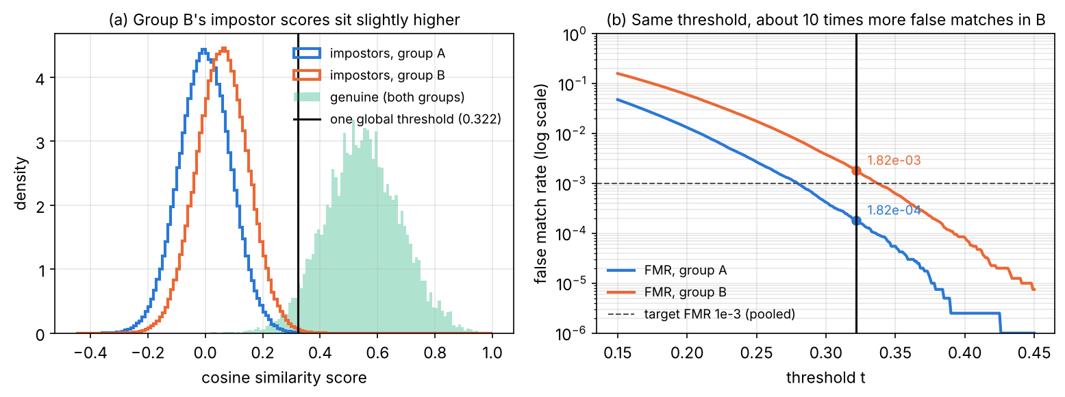
The mechanism is simple enough to simulate. Assume two groups A and B with identical genuine score distributions, but B’s impostor scores are slightly higher: different members of B look a little more alike to the network. In this toy we simply assume the shift; in real systems its causes have to be investigated. Set one global threshold for FMR = on the pooled impostors.
Code · Python · 17 lines
import numpy as np

rng = np.random.default_rng(0)
n_imp, n_gen = 400_000, 4_000
# Same genuine distribution; group B's impostor scores sit slightly higher.
imp = {"A": rng.normal(0.00, 0.09, n_imp), "B": rng.normal(0.06, 0.09, n_imp)}
gen = {"A": rng.normal(0.55, 0.13, n_gen), "B": rng.normal(0.55, 0.13, n_gen)}

pooled = np.r_[imp["A"], imp["B"]]
t_global = np.quantile(pooled, 1 - 1e-3)          # FMR = 0.1% on the pooled data
print(f"global threshold {t_global:.3f}")
for g in "AB":
    print(f"  group {g}: FMR {(imp[g] >= t_global).mean():.5f}, "
          f"FNMR {(gen[g] < t_global).mean():.4f}")
for g in "AB":
    t_g = np.quantile(imp[g], 1 - 1e-3)             # per-group threshold, FMR 0.1% each
    print(f"group {g} own threshold {t_g:.3f}: FNMR {(gen[g] < t_g).mean():.4f}")
Output
global threshold 0.322
  group A: FMR 0.00018, FNMR 0.0403
  group B: FMR 0.00182, FNMR 0.0400
group A own threshold 0.279: FNMR 0.0210
group B own threshold 0.337: FNMR 0.0517
A shift of 0.06 in the mean impostor score, two-thirds of one standard deviation, makes group B’s false match rate 10 times group A’s at the same threshold (0.182% against 0.018%), although the two groups’ false non-match rates are equal. Choosing a separate threshold per group equalizes FMR, but then group B’s FNMR rises to 5.2% while A’s falls to 2.1%: one error rate or the other differs. Which trade-off is acceptable is a policy and legal question, not a purely technical one, and group-specific thresholds raise their own concerns. The technical lessons are firmer: measure both error rates per group at the operating threshold, on data like the deployment data, and remember that the overall FAR can hide a tenfold difference (Figure 7).
Presentation attacks
Plain version. A recognition network answers “who is this?”, not “is this a real, live face?”. A printed photo, a phone screen showing a video, or a mask can be presented to the camera. Detecting such attacks is a separate task.
A presentation attack is an attempt to fool the sensor with an artifact; presentation attack detection (PAD), also called face anti-spoofing, decides whether the input is bona fide (a live person) or an attack. Yu et al. survey deep-learning methods for it [37]: beyond binary “live versus attack” labels, many methods use pixel-wise auxiliary supervision such as pseudo depth maps; the field now emphasizes domain generalization (attacks, cameras and lighting not seen in training) and open-set attacks of new types; and multi-modal sensors (depth, infrared) or special sensors (light field, flash) help. PAD runs alongside recognition, and the two error types are evaluated separately; a strong recognizer with no PAD is easy to fool with a good photo of the enrolled person. Digital attacks such as morphed passport photos and deepfakes are related but distinct threats.
Privacy, consent and the law
Plain version. A face embedding is a biometric identifier: it can link a person’s photos across the internet and cameras, and a person cannot change their face the way they change a password. Many legal systems therefore treat it as sensitive data. This section describes the context; it is not legal advice.
Two points from European law illustrate how regulators view face recognition (rules differ between jurisdictions, and they change):
- Under the EU’s General Data Protection Regulation, “biometric data for the purpose of uniquely identifying a natural person” is one of the categories of sensitive personal data, which are subject to specific processing conditions (GDPR Article 9) [38].
- The EU AI Act (Regulation (EU) 2024/1689) lists among its prohibited practices the untargeted scraping of the internet or CCTV material to create or expand facial recognition databases, and real-time remote biometric identification for law enforcement purposes in publicly accessible spaces; the prohibitions apply from 2 February 2025 [39]. The Regulation itself defines the exact scope and conditions.
For engineers, the practical consequences are concrete. Know where every training image came from and under what terms; the withdrawn datasets above show that “publicly visible” is not the same as “available for any use”. Treat stored templates as sensitive data: limit who can query a gallery, log searches, and delete templates that are no longer needed. Prefer designs that keep templates on the user’s device for verification when the application allows it. Document the intended use and the measured error rates per group, as recommended by NIST [2]. Synthetic training data [31], [33] reduces, but does not remove, these concerns, because the deployed system still processes real faces.
Failure modes and practical advice
Plain version. Most failures come from a mismatch between the conditions in training and testing: a face turned away, half covered, much older, blurred, or from a population the system rarely saw. A threshold tuned in one setting silently changes meaning in another.
- Pose. Large yaw (profile views) breaks five-point alignment and removes half the face. IJB-B was built with human-labeled face boxes precisely because datasets filtered by a commodity face detector under-represent such poses and occlusions [27], and the ArcFace authors cite pose and age gaps as conditions where plain softmax features degrade [16].
- Occlusion. Masks, sunglasses, hands and hair hide parts of the face; detectors may still fire but landmarks drift, and the embedding moves toward the impostor region.
- Age. Templates enrolled years earlier match less well; MegaFace evaluated performance with respect to age [24], and NIST found elevated false positives for the elderly and children [2].
- Image quality. Low resolution, motion blur, compression and poor lighting raise false non-matches; NIST linked several false-negative differentials to image quality rather than to demographics [2]. Quality-aware methods (MagFace, AdaFace [19], [20]) and quality checks at capture time help.
- Threshold drift. A threshold chosen on one dataset gives a different FAR on another camera, population or gallery size (Figures 6 and 7). Recalibrate on deployment-like impostor pairs, and monitor score distributions after deployment, as in ML 11.
- Label noise and identity overlap. Web-collected training sets contain mislabeled images and the same person under two names; sub-center ArcFace [18] and dataset cleaning [29] target this. Overlap between training identities and test identities inflates open-set results, so check it before reporting.
- Evaluation shortcuts. Reporting only accuracy on LFW, only rank-1 on a small closed gallery, or only one error rate hides exactly the failures above.
Modern view
What the surveys say
Wang and Deng’s survey [1] is the standard map of deep face recognition. It sorts the losses into Euclidean-distance-based (contrastive, triplet, center loss), angular/cosine-margin-based (SphereFace, CosFace, ArcFace) and softmax variations (feature and weight normalization), and it traces how Euclidean-distance-based losses dominated the early years and how angular/cosine-margin losses and feature and weight normalization took over from 2017. Drozdowski et al. [36] survey demographic bias across biometrics: how bias is estimated, how it might be mitigated, and the social and technical questions that remain. Yu et al. [37] survey deep face anti-spoofing, including methods designed for domain generalization and open-set attacks. Boutros et al. [33] survey synthetic data for face recognition, organize its use cases and discuss the challenges that remain.
Optional: Guide to the Modern view surveys (in the Paper guides). What each survey covers, how it is organized and how to use it as a map.
The state of the art, 2023–2026
- Margin-based softmax losses on very large datasets remain the standard recipe. The main changes since ArcFace are adaptive margins tied to image quality (MagFace [19], AdaFace [20]), robustness to label noise (sub-center ArcFace [18]) and efficient training over millions of identities (Partial FC [21], applied with both CNN and ViT backbones).
- Benchmarks moved to low-FAR, template-based and operational evaluation. LFW is saturated [31]; IJB-B/C at TAR@FAR = became the academic norm [16], and NIST’s FRTE (the evaluation known as FRVT until 2023 [3]) tests submitted algorithms on large operational data at false match rates as low as .
- Synthetic and privacy-aware training data is an active direction, with graphics-rendered (DigiFace-1M [31]) and diffusion-generated (DCFace [32]) datasets, motivated by consent, bias and label-noise problems of web data [33].
- Fairness is measured and reported, not assumed: NIST’s demographic analysis [2] and dedicated test sets such as RFW [34] made per-group error rates part of evaluation.
Open problems
- Generalization to unseen conditions: extreme pose, occlusion, very low resolution and long age gaps.
- Demographic differentials: measuring both error types per group on deployment-like data, and reducing differentials without simply moving errors from one group to another.
- Training data without consent problems that still reaches the accuracy of web-scale real data [33].
- Presentation and digital attacks of types not seen in training [37].
- Calibrated, quality-aware scores, so that a threshold keeps its meaning across cameras and populations.
- Governance: dataset stewardship after release [30], and legal limits that differ between jurisdictions [38], [39].
Key takeaways
- Embeddings support comparison with identities absent from training; classification labels alone do not.
- State the recognition task and gallery size before selecting metrics or thresholds.
- Detection and alignment errors propagate into embedding comparisons.
- Pair-based losses require informative samples; margin losses shape separation around class centers.
- Report verification TAR at a stated FAR and impostor-pair count; use task-specific identification metrics for search.
- Check errors by group and operating condition, verify dataset availability, and protect biometric templates.
Exercises
- Open or closed? For each system, say whether it performs verification, closed-set identification or open-set identification, and which error matters most: (a) unlocking a phone, (b) sorting a family’s photo album into its five members, (c) searching a watch list of 10,000 people at a stadium entrance.
Hint
(a) Verification; a false accept is a security failure, a false reject is an inconvenience (the user can retry). (b) Closed-set identification only if every photo shows one of the five; real albums contain guests, so it is open-set in practice. (c) Open-set identification; most people passing are not on the list, so FPIR at the chosen threshold, multiplied by the number of people passing, gives the number of false alarms.
- The ArcFace boundary. Two class centers are apart. For a feature on the arc between them, find the angle from at which class 1’s loss stops being satisfied for normalized softmax, ArcFace with rad and SphereFace with . Which margin is largest here, and what happens to SphereFace’s margin when ?
Hint
Softmax: . ArcFace: , so the gap is . SphereFace: , gap . At SphereFace’s gap doubles to , while ArcFace’s stays .
- CosFace in the toy. Change the toy experiment so that the target logit is with (CosFace). What is now? Run it and compare the three printed numbers with ArcFace’s.
Hint
Replace np.cos(th + margin) with np.cos(th) - margin in the logits, and the gradient factor np.sin(th + margin) / np.sin(th) with 1 (the derivative of with respect to is 1, so the whole factor is just ). Expect a result close to ArcFace’s; the exact numbers depend on the run.
- How many impostor pairs? You want to claim FAR = . (a) With 300,000 impostor pairs and zero false accepts observed, what is the approximate 95% upper bound on the true FAR? (b) How many impostor pairs do you need for the bound to reach with zero errors? (c) Why might your pairs be worth fewer “independent trials” than their count?
Hint
(a) Rule of three: about . (b) About 300,000, but only if no errors occur; with a few errors you need more. (c) Pairs that reuse the same images or the same people are correlated: one unusual image can produce many false accepts at once.
- Gallery growth. In the identification code, a non-mated probe at threshold 0.36 triggers a false hit with probability 0.010 for a gallery of 300. Use to estimate the per-comparison FMR, then predict FPIR for galleries of 3,000 and 30,000. Compare with the printed values and explain any difference.
Hint
gives , predicting about 0.096 for 3,000 and 0.64 for 30,000. The printed 0.043 and 0.330 are lower. With only 300 non-mated probes, an FPIR of 0.010 is just 3 false hits, so the FMR estimate is very uncertain; estimate FMR directly from many impostor comparisons instead.
- Fair thresholds. In the two-group code, find the single threshold that equalizes the two groups’ FNMR, and one that makes FMR equal. Can one threshold do both? What would you report to a decision maker?
Hint
Because the genuine distributions are identical, any single threshold gives equal FNMR (up to sampling noise: 0.0403 against 0.0400 in the printed run); no single threshold gives equal FMR, because the impostor distributions differ. Report both error rates for both groups at the proposed threshold, and the alternatives (group thresholds, a better model), and leave the choice of trade-off to the people accountable for it.
References
- M. Wang and W. Deng, “Deep face recognition: A survey,” Neurocomputing, vol. 429, pp. 215–244, 2021. doi
- P. Grother, M. Ngan and K. Hanaoka, “Face Recognition Vendor Test (FRVT) Part 3: Demographic Effects,” NIST Interagency Report 8280, National Institute of Standards and Technology, 2019. doi
- National Institute of Standards and Technology, “Face Recognition Technology Evaluation (FRTE) 1:1 Verification,” evaluation web page, accessed 2026. NIST
- K. Zhang, Z. Zhang, Z. Li and Y. Qiao, “Joint face detection and alignment using multitask cascaded convolutional networks,” IEEE Signal Processing Letters, vol. 23, no. 10, pp. 1499–1503, 2016. doi
- J. Deng, J. Guo, E. Ververas, I. Kotsia and S. Zafeiriou, “RetinaFace: Single-shot multi-level face localisation in the wild,” in Proc. IEEE/CVF CVPR, 2020. CVF
- Y. Taigman, M. Yang, M. Ranzato and L. Wolf, “DeepFace: Closing the gap to human-level performance in face verification,” in Proc. IEEE CVPR, 2014. CVF
- F. Schroff, D. Kalenichenko and J. Philbin, “FaceNet: A unified embedding for face recognition and clustering,” in Proc. IEEE CVPR, 2015. CVF
- S. Chopra, R. Hadsell and Y. LeCun, “Learning a similarity metric discriminatively, with application to face verification,” in Proc. IEEE CVPR, vol. 1, pp. 539–546, 2005. doi
- R. Hadsell, S. Chopra and Y. LeCun, “Dimensionality reduction by learning an invariant mapping,” in Proc. IEEE CVPR, vol. 2, pp. 1735–1742, 2006. doi
- A. Hermans, L. Beyer and B. Leibe, “In defense of the triplet loss for person re-identification,” arXiv:1703.07737, 2017. arXiv
- F. Wang, X. Xiang, J. Cheng and A. L. Yuille, “NormFace: L2 hypersphere embedding for face verification,” in Proc. ACM International Conference on Multimedia, pp. 1041–1049, 2017. doi
- W. Liu, Y. Wen, Z. Yu, M. Li, B. Raj and L. Song, “SphereFace: Deep hypersphere embedding for face recognition,” in Proc. IEEE CVPR, 2017. CVF
- H. Wang, Y. Wang, Z. Zhou, X. Ji, D. Gong, J. Zhou, Z. Li and W. Liu, “CosFace: Large margin cosine loss for deep face recognition,” in Proc. IEEE/CVF CVPR, 2018. CVF
- F. Wang, J. Cheng, W. Liu and H. Liu, “Additive margin softmax for face verification,” IEEE Signal Processing Letters, vol. 25, no. 7, pp. 926–930, 2018. doi
- J. Deng, J. Guo, N. Xue and S. Zafeiriou, “ArcFace: Additive angular margin loss for deep face recognition,” in Proc. IEEE/CVF CVPR, 2019. CVF
- J. Deng, J. Guo, J. Yang, N. Xue, I. Kotsia and S. Zafeiriou, “ArcFace: Additive angular margin loss for deep face recognition,” IEEE Transactions on Pattern Analysis and Machine Intelligence, vol. 44, no. 10, pp. 5962–5979, 2022. doi
- Y. Wen, K. Zhang, Z. Li and Y. Qiao, “A discriminative feature learning approach for deep face recognition,” in Proc. ECCV, pp. 499–515, 2016. doi
- J. Deng, J. Guo, T. Liu, M. Gong and S. Zafeiriou, “Sub-center ArcFace: Boosting face recognition by large-scale noisy web faces,” in Proc. ECCV, pp. 741–757, 2020. doi
- Q. Meng, S. Zhao, Z. Huang and F. Zhou, “MagFace: A universal representation for face recognition and quality assessment,” in Proc. IEEE/CVF CVPR, 2021. CVF
- M. Kim, A. K. Jain and X. Liu, “AdaFace: Quality adaptive margin for face recognition,” in Proc. IEEE/CVF CVPR, 2022. CVF
- X. An, J. Deng, J. Guo, Z. Feng, X. Zhu, J. Yang and T. Liu, “Killing two birds with one stone: Efficient and robust training of face recognition CNNs by Partial FC,” in Proc. IEEE/CVF CVPR, 2022. CVF
- A. Martin, G. Doddington, T. Kamm, M. Ordowski and M. Przybocki, “The DET curve in assessment of detection task performance,” in Proc. Eurospeech, pp. 1895–1898, 1997. ISCA
- G. B. Huang, M. Mattar, T. Berg and E. Learned-Miller, “Labeled Faces in the Wild: A database for studying face recognition in unconstrained environments,” in Workshop on Faces in ‘Real-Life’ Images: Detection, Alignment, and Recognition, Marseille, 2008. HAL
- I. Kemelmacher-Shlizerman, S. M. Seitz, D. Miller and E. Brossard, “The MegaFace benchmark: 1 million faces for recognition at scale,” in Proc. IEEE CVPR, 2016. CVF
- University of Washington, “MegaFace and MF2: Million-scale face recognition,” project web page, accessed 2026. project page
- Y. Guo, L. Zhang, Y. Hu, X. He and J. Gao, “MS-Celeb-1M: A dataset and benchmark for large-scale face recognition,” in Proc. ECCV, pp. 87–102, 2016. doi
- C. Whitelam, E. Taborsky, A. Blanton, B. Maze, J. Adams, T. Miller, N. Kalka, A. K. Jain, J. A. Duncan, K. Allen, J. Cheney and P. Grother, “IARPA Janus Benchmark-B face dataset,” in Proc. IEEE CVPR Workshops, 2017. CVF
- B. Maze, J. Adams, J. A. Duncan, N. Kalka, T. Miller, C. Otto, A. K. Jain, W. T. Niggel, J. Anderson, J. Cheney and P. Grother, “IARPA Janus Benchmark – C: Face dataset and protocol,” in Proc. International Conference on Biometrics (ICB), pp. 158–165, 2018. doi
- Z. Zhu, G. Huang, J. Deng, Y. Ye, J. Huang, X. Chen, J. Zhu, T. Yang, J. Lu, D. Du and J. Zhou, “WebFace260M: A benchmark unveiling the power of million-scale deep face recognition,” in Proc. IEEE/CVF CVPR, 2021. CVF
- K. Peng, A. Mathur and A. Narayanan, “Mitigating dataset harms requires stewardship: Lessons from 1000 papers,” in Proc. NeurIPS Datasets and Benchmarks Track, 2021. proceedings
- G. Bae, M. de La Gorce, T. Baltrušaitis, C. Hewitt, D. Chen, J. Valentin, R. Cipolla and J. Shen, “DigiFace-1M: 1 million digital face images for face recognition,” in Proc. IEEE/CVF WACV, 2023. CVF
- M. Kim, F. Liu, A. Jain and X. Liu, “DCFace: Synthetic face generation with dual condition diffusion model,” in Proc. IEEE/CVF CVPR, 2023. CVF
- F. Boutros, V. Struc, J. Fierrez and N. Damer, “Synthetic data for face recognition: Current state and future prospects,” Image and Vision Computing, vol. 135, art. 104688, 2023. doi
- M. Wang, W. Deng, J. Hu, X. Tao and Y. Huang, “Racial Faces in the Wild: Reducing racial bias by information maximization adaptation network,” in Proc. IEEE/CVF ICCV, pp. 692–702, 2019. doi
- J. Buolamwini and T. Gebru, “Gender Shades: Intersectional accuracy disparities in commercial gender classification,” in Proc. Conference on Fairness, Accountability and Transparency, PMLR 81, pp. 77–91, 2018. PMLR
- P. Drozdowski, C. Rathgeb, A. Dantcheva, N. Damer and C. Busch, “Demographic bias in biometrics: A survey on an emerging challenge,” IEEE Transactions on Technology and Society, vol. 1, no. 2, pp. 89–103, 2020. doi
- Z. Yu, Y. Qin, X. Li, C. Zhao, Z. Lei and G. Zhao, “Deep learning for face anti-spoofing: A survey,” IEEE Transactions on Pattern Analysis and Machine Intelligence, vol. 45, pp. 5609–5631, 2023. doi
- European Commission, “What personal data is considered sensitive?,” data protection guidance referring to Article 9 of the GDPR, accessed 2026. European Commission
- European Commission, “AI Act” (Regulation (EU) 2024/1689), policy page, accessed 2026. European Commission
- M. Turk and A. Pentland, “Eigenfaces for recognition,” Journal of Cognitive Neuroscience, vol. 3, no. 1, pp. 71–86, 1991. doi
- P. N. Belhumeur, J. P. Hespanha and D. J. Kriegman, “Eigenfaces vs. Fisherfaces: Recognition using class specific linear projection,” IEEE Transactions on Pattern Analysis and Machine Intelligence, vol. 19, no. 7, pp. 711–720, 1997. doi
Check your understanding
This tutorial has 6 exercises. Can you solve them without opening the hints?
Go to the exercises ↑Next DLCV 03 · Object Detection: From R-CNN to DETR · 34 min