DLCV 01B · Building Blocks and How to Compose Them: Classification and Restoration Networks
Needs: DLCV 01 · Deep Learning for Image Processing and Computer Vision, ML 05 · Attention and Vision Transformers
Navigate: this page and this track: Navigate: this page and this track
On this page
- What you’ll learn1 min
- The big picture1 min
- Anatomy of a network3 min
- The block catalogue18 min
- Composing for classification3 min
- Composing for restoration3 min
- Side by side: what changed and why4 min
- Exploring a design space4 min
- Common composition mistakes1 min
- Modern view3 min
- Key takeaways1 min
- Exercises3 min
- Supplementary notes
- Paper guides
- References
Deep Learning for Computer Vision
What you’ll learn
- Identify a network’s stem, stages, blocks, neck and head.
- Track how blocks mix spatial and channel information, and estimate their costs.
- Explain why classification and restoration use resolution, normalization and skips differently.
- Compare matched network designs and diagnose composition errors with small experiments.
- Read ablations under controlled training and compute budgets.
The big picture
A vision network looks complicated in a paper figure, but it is built from a small number of block types, repeated and connected. Two networks that use the same blocks can behave very differently because they are composed differently: where the resolution changes, where the skips go, where normalization sits, how the output is formed. This chapter is about those composition decisions.
Why it matters. Practical work is rarely inventing a block. It is choosing a backbone, adapting it to a new task, or deciding which of a paper’s ten changes actually helped. A classifier backbone used unchanged for denoising throws away detail, and a block that helped in one paper may not help in your design space.
Where the basics are. The blocks themselves are taught elsewhere on this site, and this chapter links there instead of repeating them: convolution, receptive field and residual blocks in ML 03 and DLCV 01; the Transformer block, Swin and efficient attention in ML 05; the classification backbones in DLCV 02; encoder–decoders and ASPP in DLCV 04; restoration backbones and upsampling in DLCV 09 and DLCV 09A. All code here uses NumPy and SciPy only, runs on a CPU in seconds, and uses synthetic data or skimage.data.
Anatomy of a network
Plain version. A vision network usually has a stem that extracts features, a body of repeated blocks and a task head. Follow resolution changes through all three.
Precise version. Write a feature map as a tensor of shape , where is the number of channels (the width) and the spatial size. The common parts are:
- Stem: the first one or two layers. ResNet uses a convolution with stride 2 and a max-pool with stride 2, so the body starts at of the input resolution [1]. ConvNeXt replaces this with a “patchify” convolution with stride 4 [2]; ViT cuts the image into patches [3]. Restoration networks use a single convolution at full resolution, which SwinIR calls shallow feature extraction [4].
- Stage: a run of blocks that share one resolution and one width. A block is the repeated unit (a residual block, a Transformer block).
- Downsampling layer (transition): halves and , usually while doubling . It can be a strided convolution inside the first block of a stage (ResNet), a separate convolution with stride 2 (ConvNeXt, NAFNet), patch merging (Swin), or pixel unshuffle (Restormer).
- Neck: an optional module that mixes features from several stages, such as the Feature Pyramid Network (FPN) used by detectors [5].
- Head: global average pooling and a linear layer for classification; a final convolution, and for super-resolution an upsampler, for restoration.
The output stride of a stage is the ratio between the input size and the stage’s feature-map size. ResNet’s four stages have output strides 4, 8, 16 and 32 [1]; so do Swin’s [6]. Networks that keep one resolution and width throughout, like ViT, are isotropic; those with stages at decreasing resolution are hierarchical.
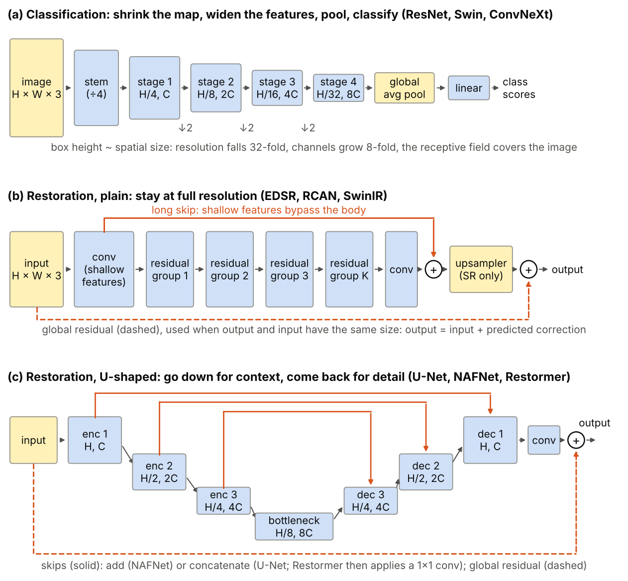
ResNet also states the most copied rule of macro design: when the feature map is halved, the number of filters is doubled “so as to preserve the time complexity per layer” [1]. A convolution with input and output channels on an map costs multiply-accumulates (MACs); after halving the map and doubling the width it costs , the same. Figure 1 shows the three macro-architectures this chapter compares.
The block catalogue
Plain version. Blocks mix information across space and channels. Skips, normalization and nonlinearities control how that mixing affects the signal and its cost.
The MetaFormer paper makes this split explicit: a Transformer block is a token mixer (attention) followed by a channel mixer (the MLP), each in a residual branch with normalization, and replacing attention by a simple spatial pooling operator still gave competitive accuracy on ImageNet [7], which suggests that the general structure carries much of the performance [8]. Figure 2 shows the blocks of this chapter in that common format.
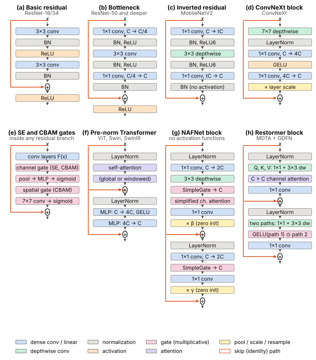
The table gives each block one plain line and says where its basics are taught.
| Block | One plain line | Used in | Basics |
|---|---|---|---|
| Residual (basic) | Learn a correction and add it to the input | ResNet-18/34, EDSR | DLCV 01 |
| Bottleneck | Squeeze channels with , filter, expand back | ResNet-50 and deeper | DLCV 02 |
| Depthwise separable | Filter each channel alone, then mix channels with | MobileNet [9] | DLCV 02 |
| Inverted residual | Expand, filter depthwise, project back linearly; skip between thin ends | MobileNetV2 [10] | ML 03 |
| ConvNeXt block | Large depthwise kernel, then a Transformer-style MLP | ConvNeXt | DLCV 02 |
| SE / CBAM | Reweight channels (and positions) by a gate computed from pooled statistics | SENet, RCAN, NAFNet | DLCV 02 note |
| Self-attention | Every token looks at every other token | ViT | ML 05 |
| Window attention | Attention inside local windows that shift between layers | Swin, SwinIR | ML 05 |
| Channel (transposed) attention | Attention between channels, so cost grows linearly with pixels | Restormer | this chapter |
| Gated block | Multiply two feature halves instead of applying an activation | NAFNet, Restormer’s GDFN | this chapter |
Residual connections and residual scaling
Plain version. A residual block adds a learned correction to its input. Check normalization, activation placement and the correction’s initial scale.
Precise version. The general form is
where is the block input, the residual branch (convolutions, attention, normalization), the output and a scale on the branch. Three placements of the nonlinearity are common:
- Post-activation (original ResNet): , with BN inside [1].
- Pre-activation: BN and ReLU move inside the branch, before each convolution, so the shortcut is a pure identity; He et al. found this easier to train at very large depth [11]. The pre-norm Transformer block, , is the same idea (ML 05).
- No activation after the addition: EDSR, MobileNetV2, ConvNeXt, NAFNet and Restormer all end the block with the addition.
Several designs control explicitly. EDSR found training numerically unstable once the number of feature maps grew large, and fixed it with a constant residual scaling of 0.1 in its final model of 32 blocks with 256 channels [12]. ConvNeXt uses Layer Scale [13], a learnable per-channel , initialized to [2]. NAFNet’s code multiplies each branch by learnable per-channel parameters initialized to zero, so every block starts as the identity [14]; zero-initializing the last BN scale of a ResNet branch does the same (DLCV 01A). The shared reason: a deep stack of identity blocks is easy to optimize, and each block can then grow its correction.
Skips also come at two scales. Short skips wrap one block; long skips wrap a group of blocks or the whole body. RCAN’s “residual in residual” structure uses both: residual groups with long skip connections, each containing blocks with short skip connections [15].
Training and inference can also use different block graphs: RepVGG [54] trains with additional affine branches and converts them into one convolution for deployment.
Optional: RepVGG: training with branches, deploying a plain network (in the Paper guides). The exact conversion, architecture choices and measured trade-offs.
Bottlenecks, inverted residuals and depthwise separable convolutions
Plain version. Spatial filtering and channel mixing need not happen in one expensive layer. Bottlenecks run the expensive on fewer channels; depthwise convolutions filter each channel alone and leave mixing to cheap layers. These blocks change cost by large factors, so it pays to count.
Precise version. A dense convolution from to channels has weights and, at stride 1, costs MACs per output pixel. A depthwise convolution on channels has of each. The ResNet bottleneck reduces to , filters, and expands back [1]. The MobileNetV2 inverted residual does the opposite: it expands to with a convolution (expansion factor in the paper’s main experiments), filters with a depthwise convolution, and projects back with a linear convolution, without an activation, because the authors argue that a ReLU in the narrow layer destroys information [10]. The paper gives its cost as multiply-adds for an input with input and output channels [10]. The snippet counts weights and MACs per output pixel for the blocks of Figure 2 at , on a map, and checks the inverted residual against that formula.
Code · Python · 26 lines
# Weights (no biases or norm parameters) and MACs per output pixel of common blocks,
# all with C input and C output channels at stride 1. A dense k x k conv from a to b
# channels has k*k*a*b weights and costs k*k*a*b MACs per pixel; a depthwise one k*k*a.
def blocks(C, n_tokens):
    g = int(2.66 * C)                                  # Restormer GDFN hidden width
    return {                                           # name: (weights, MACs per pixel)
        'basic residual (2 x 3x3)':     (18 * C * C, 18 * C * C),
        'bottleneck (1x1, 3x3, 1x1)':   (2 * C * C // 4 + 9 * (C // 4) ** 2,) * 2,
        'depthwise separable 3x3':      (9 * C + C * C,) * 2,
        'inverted residual, t = 6':     (12 * C * C + 54 * C,) * 2,
        'ConvNeXt (7x7 dw, 4x MLP)':    (49 * C + 8 * C * C,) * 2,
        'NAFNet block':                 (7 * C * C + 18 * C, 6 * C * C + 18 * C),  # SCA acts on a pooled vector
        'SE add-on, r = 16':            (2 * C * C // 16, C),                       # one multiply per pixel
        'ViT block, global attention':  (12 * C * C, 12 * C * C + 2 * n_tokens * C),
        'Swin block, 8 x 8 windows':    (12 * C * C, 12 * C * C + 2 * 64 * C),
        'Restormer block (MDTA+GDFN)':  (4 * C * C + 27 * C + 3 * g * C + 18 * g,
                                         4 * C * C + 27 * C + 2 * C * C // 4 + 3 * g * C + 18 * g),  # 4 heads
    }

C, side = 64, 128
for name, (p, m) in blocks(C, side * side).items():
    print(f"{name:30s} {p:7d} weights  {m:8d} MACs/pixel")

# Check the inverted residual against MobileNetV2's formula h*w*d'*t*(d' + k^2 + d'') per pixel.
t, k = 6, 3
assert blocks(C, 1)['inverted residual, t = 6'][1] == C * t * (C + k * k + C)
Output
basic residual (2 x 3x3)         73728 weights     73728 MACs/pixel
bottleneck (1x1, 3x3, 1x1)        4352 weights      4352 MACs/pixel
depthwise separable 3x3           4672 weights      4672 MACs/pixel
inverted residual, t = 6         52608 weights     52608 MACs/pixel
ConvNeXt (7x7 dw, 4x MLP)        35904 weights     35904 MACs/pixel
NAFNet block                     29824 weights     25728 MACs/pixel
SE add-on, r = 16                  512 weights        64 MACs/pixel
ViT block, global attention      49152 weights   2146304 MACs/pixel
Swin block, 8 x 8 windows        49152 weights     57344 MACs/pixel
Restormer block (MDTA+GDFN)      53812 weights     55860 MACs/pixel
Four lessons come out of these numbers.
- At equal width, the blocks differ by more than 10 times in cost. The bottleneck and the separable block are about 16 to 17 times cheaper than the basic block. Real networks therefore never compare blocks at equal width: MobileNetV2 uses an inverted residual on thin tensors, ResNet-50 uses bottlenecks on wide ones. Compare blocks at equal cost, not at equal .
- Global attention over pixels is out of reach for restoration. With every pixel of a map as a token, the ViT block costs about 37 times more per pixel than a Swin block with windows, and the gap grows with image size. This is why restoration Transformers use windows (SwinIR) or attention across channels (Restormer); see ML 05 for the general cost argument.
- Attention add-ons are cheap in MACs. An SE gate adds weights and one multiply per channel and pixel; its cost is memory traffic, not arithmetic.
- MACs are not latency. Depthwise layers do few operations per byte moved, so they can run slower than their MAC count suggests; ML 03 and the DLCV 02 efficiency section discuss this. Measure on the target hardware.
Whether a cheaper block is also a better one depends on the design space. RegNet’s population study found that its best models used neither a bottleneck nor an inverted bottleneck, and that depthwise convolution did even worse than the inverted bottleneck in its setting [16], while ConvNeXt found the inverted bottleneck slightly better within its own sequence of changes [2]. Both can be true: the comparison depends on the other choices held fixed.
Attention inside a CNN: SE and CBAM
Plain version. A gate looks at a summary of the whole feature map and decides which channels (or positions) to turn up or down for this particular image. It is a cheap way to give a convolutional network some content-dependent, image-wide behavior.
Precise version. Squeeze-and-excitation (SE) computes a channel gate from the vector of channel means, where and are the weights of a two-layer MLP that shrinks the dimension by a ratio and restores it, is a ReLU and the sigmoid, and multiplies each channel of the feature map by ; the formula and code are in the DLCV 02 note [17]. CBAM extends it in two ways [18]: its channel gate pools each channel by both average and maximum and passes both vectors through one shared MLP, and a second, spatial gate pools across channels and applies a convolution, so the block can also turn whole regions up or down. CBAM’s ablations found the sequential channel-then-spatial order better than running the two gates in parallel [18].
Optional: CBAM’s channel and spatial gates (in the Supplementary notes). The two formulas with every symbol defined, and how they relate to SE and to NAFNet’s simplified channel attention.
Where it goes. Both SE and CBAM sit on the residual branch, before the addition: SE applies the gate to the non-identity branch “before summation with the identity branch” [17], and CBAM applies its module to the convolution outputs of each ResNet block [18]. RCAN brought channel attention into super-resolution [15]; NAFNet later simplified it to , a single linear map of the pooled vector with no ReLU or sigmoid, and lost nothing in its ablation [19]. The Modern view’s attention survey places SE in the “channel attention” family and CBAM in “channel and spatial” [20].
Token mixers: self-, window- and channel attention
Plain version. Attention mixes information between tokens with weights computed from the content, instead of fixed weights as in a convolution. The design question is which tokens talk to which: all of them (global), those in the same local window, or, in Restormer’s twist, the channels instead of the pixels.
Precise version. Global multi-head self-attention over tokens of width costs about MACs for the scores and the weighted sum, on top of for the projections; window attention restricts it to windows, giving (ML 05) [6]. Restormer’s multi-Dconv head transposed attention (MDTA) instead computes attention between channels [21]:
where is the input feature map and the output, (and likewise , ) is computed from the layer-normalized input by a convolution followed by a depthwise convolution , the hats denote reshaped matrices , , , is a learnable temperature, and without a superscript is the output convolution. The attention map has size instead of , so the cost grows linearly with the number of pixels, and every output pixel still depends on the whole image through the channel statistics. The depthwise convolutions put local context back in. As in ordinary multi-head attention, the channels are split into heads with separate maps.
Restormer’s feed-forward part (GDFN) is covered with the gates below. The trade-off between the mixers returns in the restoration sections: window attention mixes space strongly but locally, channel attention reaches globally at low cost, and a comparative study argued that Restormer’s spatial mapping is weaker than SwinIR’s for super-resolution [22].
Normalization: BN, LN, GN, and when to leave it out
Plain version. A normalization layer rescales features to a standard size and then lets the network learn its preferred scale. The layers differ in which numbers share statistics. In classification the choice mostly affects training stability; in restoration the wrong choice can change the brightness and contrast of the output.
Precise version. All the common layers compute over some set of values (ML 02 gives the template). For a mini-batch of shape :
| Layer | Statistics computed over | Depends on the batch? |
|---|---|---|
| BatchNorm (BN) [23] | for each channel | yes; running averages at test time |
| LayerNorm (LN) [24] | the features of one sample (for images, implementations differ: all of , or at each position) | no |
| InstanceNorm (IN) [25] | for each sample and channel | no |
| GroupNorm (GN) [26] | and a group of channels, for each sample | no; gives LN, gives IN |
BN is the default in classification CNNs and works well with large batches. Its known failure is small batches: GN’s authors report a ResNet-50 on ImageNet with 10.6% lower error than its BN counterpart at a batch size of 2 [26]. What BN computes, and why training and inference differ, is in the DLCV 01 note.
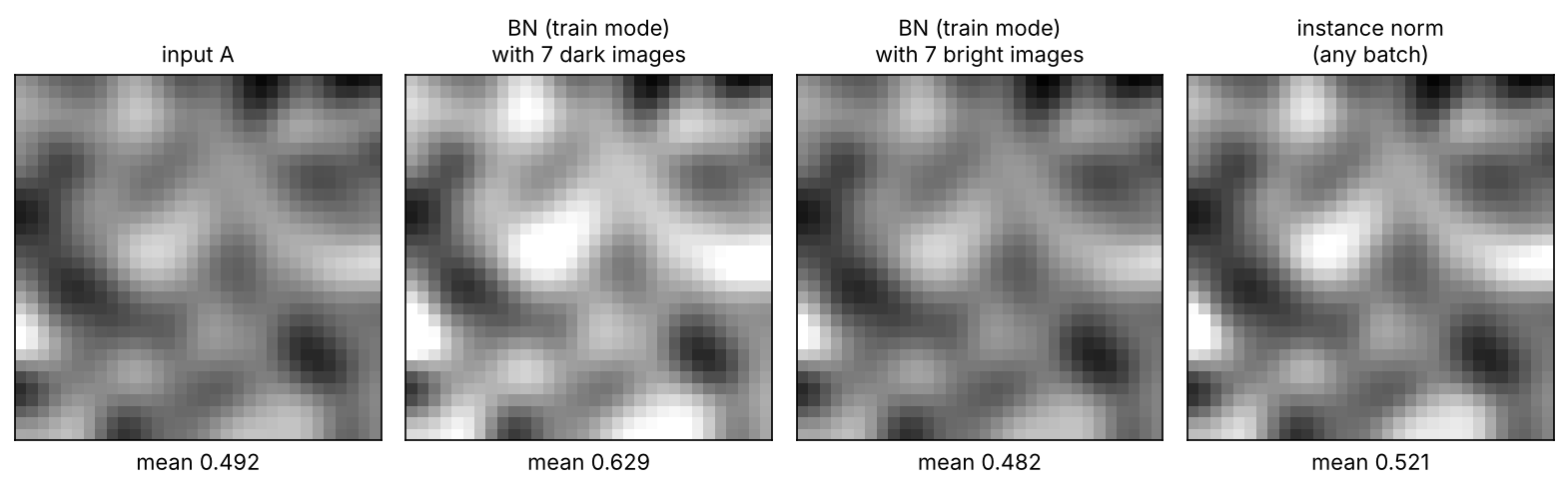
Why restorers dropped BN. EDSR removed BN from its residual blocks, arguing that because BN normalizes the features it removes “range flexibility” from the network; the change improved accuracy and cut training memory by about 40% compared with SRResNet, the residual SR network of the SRGAN paper [27], [12]. ESRGAN added that BN tends to introduce artifacts when training and test statistics differ, especially in deeper networks trained with a GAN loss, and removed it as well [28]. This is not a law: DnCNN combined residual learning with BN for Gaussian denoising and reported that the two help each other [29]. The snippet shows the mechanism with a fixed, untrained residual branch (convolution, normalization, ReLU, convolution) and the global residual . The same mid-gray image is restored inside two different batches.
Code · Python · 47 lines
import numpy as np
from scipy.ndimage import gaussian_filter, correlate

rng = np.random.default_rng(0)

def image(level, size=32):
    """A smooth synthetic image with mean brightness `level` (values roughly in [0, 1])."""
    t = gaussian_filter(rng.standard_normal((size, size)), 2)
    return level + 0.15 * t / t.std()

C = 4
W1 = rng.normal(0.1, 0.2, (C, 3, 3))           # 3x3 conv, 1 -> C channels (fixed random weights)
w2 = rng.normal(0.0, 0.05, C)                  # 1x1 conv, C -> 1 channel

def features(batch):                           # (N, H, W) -> (N, C, H, W)
    return np.stack([[correlate(x, W1[c], mode='nearest') for c in range(C)] for x in batch])

def branch(batch, norm, running=None):
    """Residual branch: conv -> normalize -> ReLU -> 1x1 conv."""
    f = features(batch)
    if norm == 'bn-train':                     # per channel, over the whole batch
        mu, var = f.mean((0, 2, 3), keepdims=True), f.var((0, 2, 3), keepdims=True)
    elif norm == 'bn-eval':                    # per channel, stored training statistics
        mu, var = running
    else:                                      # 'instance': per sample and channel
        mu, var = f.mean((2, 3), keepdims=True), f.var((2, 3), keepdims=True)
    h = np.maximum((f - mu) / np.sqrt(var + 1e-5), 0)
    return np.tensordot(w2, h, axes=(0, 1))    # (N, H, W)

train = np.stack([image(rng.uniform(0.3, 0.7)) for _ in range(64)])
f = features(train)
running = (f.mean((0, 2, 3), keepdims=True), f.var((0, 2, 3), keepdims=True))

A = image(0.5)
dark = np.stack([image(0.15) for _ in range(7)])
bright = np.stack([image(0.85) for _ in range(7)])
for norm in ['bn-train', 'bn-eval', 'instance']:
    for name, others in [('dark', dark), ('bright', bright)]:
        batch = np.concatenate([A[None], others])
        out = A + branch(batch, norm, running)[0]          # global residual: y = x + r(x)
        print(f"{norm:8s}  A with 7 {name:6s} images: output mean {out.mean():.3f}")

# Per-sample normalization forgets each image's level and contrast:
B = 0.5 * A + 0.3
r_A, r_B = branch(A[None], 'instance')[0], branch(B[None], 'instance')[0]
print("instance-norm branch, A vs 0.5*A + 0.3: max |r_A - r_B| =", np.abs(r_A - r_B).max().round(4))
print("outputs with the global residual: means", (A + r_A).mean().round(3), (B + r_B).mean().round(3))
Output
bn-train  A with 7 dark   images: output mean 0.629
bn-train  A with 7 bright images: output mean 0.482
bn-eval   A with 7 dark   images: output mean 0.509
bn-eval   A with 7 bright images: output mean 0.509
instance  A with 7 dark   images: output mean 0.521
instance  A with 7 bright images: output mean 0.521
instance-norm branch, A vs 0.5*A + 0.3: max |r_A - r_B| = 0.0005
outputs with the global residual: means 0.521 0.575
In training mode, BN gives the same image (input mean 0.492) an output brightness of 0.629 or 0.482 depending only on its batch companions (Figure 3). In evaluation mode the batch no longer matters, but the stored statistics come from other images, so the network behaves differently at test time from how it was trained: the mismatch EDSR and ESRGAN describe. Per-sample normalization is batch-independent but blind in the other direction: the branch gives the same output for and for (up to ), so only the identity path carries the image’s own level and contrast. That is why restorers that do normalize (NAFNet, Restormer and SwinIR use LayerNorm) keep it inside residual branches with a global residual [19], [21], [4]. The weights are random and untrained; training can partly compensate, but the batch dependence is structural.
NAFNet’s ablation shows the other side: adding LayerNorm to its plain block let it train with a 10 times larger learning rate and raised PSNR [30] by 0.44 dB on the SIDD denoising benchmark [31] and by 3.39 dB on the GoPro deblurring benchmark [32], [19]. Normalization helps restorers too, as long as it does not take away the information the output needs.
Activations and gates
Plain version. A nonlinearity is what lets stacked layers do more than one linear map. The classic choice applies a fixed function to every number (ReLU, GELU). A gate instead multiplies two learned features, so one feature decides how much of the other passes. Modern restoration blocks use gates and, in NAFNet’s case, nothing else.
Precise version. ReLU, GELU and the SwiGLU feed-forward block [33] are defined in ML 02. The gated linear unit (GLU) of Dauphin et al. computes with two linear maps , and a sigmoid [34]. NAFNet’s SimpleGate drops the sigmoid and the second map [19]:
where is a feature map with channels, and are its first and second channels, and is element-wise multiplication. The product of two linear functions of the input is quadratic, so the block is nonlinear without any activation function; the authors note that GELU itself, with the standard normal CDF [35], is a special case of a gate. Restormer’s GDFN uses with the GELU, two paths of and depthwise convolutions, and a channel expansion [21]. In NAFNet’s ablation, replacing GELU by SimpleGate gave +0.08 dB on SIDD and +0.41 dB on GoPro [19].
Upsampling: transposed convolution, pixel shuffle and resize-convolution
Plain version. Upsampling makes a feature map larger. There are three common ways: let each input pixel “paint” a learned patch into the output (transposed convolution), compute several values per input pixel and rearrange them (pixel shuffle), or enlarge first and convolve afterwards (resize-convolution). The first two can easily paint a regular checkerboard pattern; the third cannot.
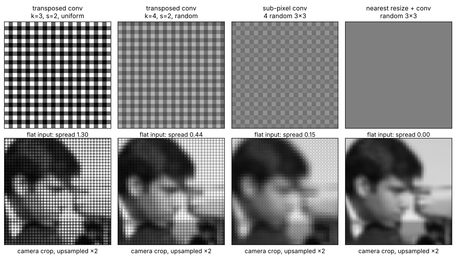
Precise version. The three methods and the exact pixel-shuffle index rule are in DLCV 09 and DLCV 09A [36]. What matters for composition is a counting argument. With stride , the output pixels fall into phases (their row and column positions modulo ). In a transposed convolution, the output at a given phase receives only some of the kernel’s taps. Its value on a flat input equals the sum of those taps, the phase sum. If the phase sums differ, a flat input comes out as a periodic pattern. One cause, which Odena et al. call uneven overlap, occurs when the kernel size is not divisible by the stride: the phases then receive different numbers of taps [37]. Even with divisible sizes, random weights give unequal phase sums, so a freshly initialized layer still makes a pattern; Aitken et al. list these two causes and strided operations in the loss as the three sources of checkerboard artifacts [38]. A sub-pixel convolution has the same freedom, since each phase has its own filter. A resize-convolution (nearest-neighbor upsampling, then an ordinary convolution) applies the same full kernel at every output pixel, so all phases see the same sum. The snippet upsamples a flat input by 2.
Code · Python · 36 lines
import numpy as np
from scipy.ndimage import correlate

rng = np.random.default_rng(0)

def transposed_conv(x, w, s):
    """Each input pixel 'paints' a scaled copy of the k x k kernel w; copies are s pixels apart."""
    k, (H, W) = w.shape[0], x.shape
    out = np.zeros((s * (H - 1) + k, s * (W - 1) + k))
    for i in range(H):
        for j in range(W):
            out[s * i:s * i + k, s * j:s * j + k] += x[i, j] * w
    return out

def resize_conv(x, w, s):
    """Nearest-neighbour upsampling by s, then an ordinary 'same' convolution with w."""
    return correlate(np.kron(x, np.ones((s, s))), w, mode='nearest')

def subpixel_conv(x, ws, s):
    """s*s ordinary convolutions whose outputs are interleaved (pixel shuffle)."""
    out = np.zeros((s * x.shape[0], s * x.shape[1]))
    for n, w in enumerate(ws):
        out[n // s::s, n % s::s] = correlate(x, w, mode='nearest')
    return out

x = np.ones((16, 16))                          # flat input: a good upsampler returns a flat image
cases = {
    'transposed k=3, s=2, uniform w': transposed_conv(x, np.ones((3, 3)), 2)[4:-4, 4:-4],
    'transposed k=4, s=2, uniform w': transposed_conv(x, np.ones((4, 4)), 2)[4:-4, 4:-4],
    'transposed k=4, s=2, random w ': transposed_conv(x, rng.uniform(0.5, 1.5, (4, 4)), 2)[4:-4, 4:-4],
    'sub-pixel, 4 random 3x3 kernels': subpixel_conv(x, rng.uniform(0.5, 1.5, (4, 3, 3)), 2)[4:-4, 4:-4],
    'resize + conv, random 3x3 w   ': resize_conv(x, rng.uniform(0.5, 1.5, (3, 3)), 2)[4:-4, 4:-4],
}
for name, y in cases.items():
    phases = [y[a::2, b::2].mean() for a in (0, 1) for b in (0, 1)]     # the four 2x2 sub-pixel phases
    print(f"{name}: phase means {np.round(phases, 2)}  relative spread {np.ptp(y) / y.mean():.2f}")
Output
transposed k=3, s=2, uniform w: phase means [4. 2. 2. 1.]  relative spread 1.30
transposed k=4, s=2, uniform w: phase means [4. 4. 4. 4.]  relative spread 0.00
transposed k=4, s=2, random w : phase means [4.04 3.22 5.01 3.85]  relative spread 0.44
sub-pixel, 4 random 3x3 kernels: phase means [ 8.71 10.13  9.49  8.91]  relative spread 0.15
resize + conv, random 3x3 w   : phase means [7.86 7.86 7.86 7.86]  relative spread 0.00
With and , one phase receives 4 taps, two receive 2 and one receives 1, even with uniform weights: the 4 : 2 : 2 : 1 pattern is built into the shapes. With every phase receives 4 taps, so uniform weights give a flat output, but random weights do not. Only resize-convolution is flat for any weights. Figure 4 shows the same four upsamplers on a flat input and on a photograph. Training can push the phase sums together, and Odena et al. report their best results with nearest-neighbor resize-convolution [37]; for pixel shuffle, initializing all phases from one kernel removes the pattern at the start [38], as noted in DLCV 09A.
Optional: Phase sums of a transposed convolution in 1-D (in the Supplementary notes). How many taps each output phase receives for any kernel size and stride, and why divisibility is necessary but not sufficient.
Downsampling has matching choices: strided convolution (ResNet), pooling, a separate convolution with stride 2 (ConvNeXt, NAFNet [14]), patch merging (Swin) and pixel unshuffle (Restormer [21]). ConvNeXt reports that its separate downsampling layers made training diverge until it added normalization layers wherever the spatial resolution changes [2].
Skip connections: add or concatenate
Plain version. A skip connection brings an earlier feature map to a later layer. It can be added (the two maps must have the same shape, and the result keeps the width) or concatenated (the maps are stacked along channels, and the next layer decides how to combine them). Concatenation is more flexible and more expensive.
Precise version. Concatenation followed by a convolution contains addition as a special case: with encoder map and decoder map , each with channels, the convolution with weight matrix (two identity blocks side by side) maps to . So concatenation can learn anything addition can, and more, at the cost of a wider layer and of storing both maps. The snippet checks the identity and counts the cost of the first convolution after each merge in a 4-level U-Net decoder with widths 32 to 256, on a input.
Code · Python · 24 lines
import numpy as np

rng = np.random.default_rng(0)

# 1) Concatenation followed by a 1x1 convolution contains addition as a special case.
C, H, W = 8, 5, 5
enc, dec = rng.standard_normal((C, H, W)), rng.standard_normal((C, H, W))
cat = np.concatenate([enc, dec])                       # (2C, H, W)
W_fuse = np.hstack([np.eye(C), np.eye(C)])             # a 1x1 conv is a (C_out x C_in) matrix
print("concat + 1x1 conv [I I] == add:", np.allclose(np.tensordot(W_fuse, cat, 1), enc + dec))

# 2) What each choice costs in the decoder of a 4-level U-Net on a 256 x 256 input.
widths, size = [32, 64, 128, 256], 256
totals = {'add': [0, 0], 'concat': [0, 0], 'concat + 1x1': [0, 0]}
for level, c in enumerate(widths):
    hw = (size // 2 ** level) ** 2                     # pixels at this level
    first = {'add': 9 * c * c,                         # first 3x3 conv after the merge
             'concat': 9 * 2 * c * c,
             'concat + 1x1': 2 * c * c + 9 * c * c}    # 1x1 halves channels, then 3x3
    for k, p in first.items():
        totals[k][0] += p
        totals[k][1] += p * hw
for k, (p, m) in totals.items():
    print(f"{k:13s} merge-layer weights {p:7d}   MACs {m / 1e9:.2f} G")
Output
concat + 1x1 conv [I I] == add: True
add           merge-layer weights  783360   MACs 2.42 G
concat        merge-layer weights 1566720   MACs 4.83 G
concat + 1x1  merge-layer weights  957440   MACs 2.95 G
Concatenating doubles the merge layer’s weights and MACs; a fusion first, as Restormer does, recovers most of the saving. The choice differs across well-known designs:
- U-Net concatenates the (cropped) encoder map with the decoder map after a up-convolution that halves the channels [39].
- FPN adds: the coarser map is upsampled by 2 with nearest-neighbor interpolation and added to a -projected backbone map, and a convolution on each merged map reduces the aliasing of the upsampling [5] (DLCV 03).
- Restormer concatenates and then halves the channels with a convolution at all levels except the top [21].
- NAFNet’s code adds the encoder map to the upsampled decoder map [14].
- DenseNet concatenates the outputs of all earlier layers in a block [40] (DLCV 02 note).
Multi-scale modules: FPN, ASPP and the U-Net
Plain version. Objects and degradations come at many sizes. Multi-scale modules let one network look at several scales at once: by building a pyramid of feature maps (FPN), by probing one map with filters of several sizes (ASPP), or by going down and back up (U-Net).
These are composition patterns more than blocks, and each is taught where it is used: FPN in DLCV 03 [5]; atrous spatial pyramid pooling (ASPP), parallel atrous convolutions at several rates, in DLCV 04 [41]; the U-Net in DLCV 01 and the IP 10 paper guide [39]. One rule connects them: context comes from going coarse, detail comes from a path that stayed fine. FPN’s lateral connections, U-Net’s skips and the low-level skip of the segmentation decoders in DLCV 03B are all that second path.
Composing for classification
Plain version. A classifier must answer one question about the whole image. So it shrinks the image quickly, spends its computation on small, wide feature maps where each position already sees a large region, and finally throws away the spatial grid altogether.
The principles, with the reason for each:
- Downsample early with a stem. The first layers run on the most pixels, so the stem cuts the resolution by 4 before the body starts (ResNet’s stride-2 convolution plus max-pool [1]; ConvNeXt’s stride-4 patchify layer, which cost nothing in accuracy in its roadmap [2]).
- Halve the resolution and double the width at each stage. This keeps the cost per layer roughly constant (see the anatomy section) and grows the receptive field geometrically.
- Put most blocks in the third stage. ResNet-50 uses (3, 4, 6, 3) blocks per stage; ConvNeXt changed this to (3, 3, 9, 3), following Swin’s 1:1:3:1 ratio, and gained accuracy [2]. The third stage, at output stride 16, has a large receptive field and still enough positions.
- Pool globally, then classify linearly. Global average pooling makes the output invariant to where the object is and lets the network accept any input size. The ViT paper found that a class token and global average pooling work similarly well, but need different learning rates [3].
- Put expensive global mixing where tokens are few. Global attention is affordable in late stages; hybrid designs put convolutions early and attention late (ML 05). Cheap gates like SE can go in every block.
- Batch normalization is fine when batches are large; use GN or LN when they are not.
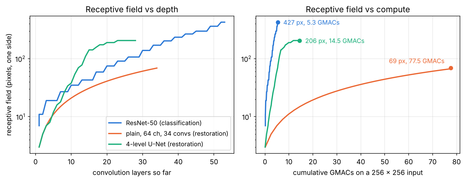
How fast does the receptive field grow? The recurrence of ML 03 covers strided stacks; the snippet also handles upsampling by walking back from one output unit and tracking the interval of inputs that reach it. It compares ResNet-50 with two restorers on a input: a plain full-resolution body of the EDSR-baseline shape (16 residual blocks of two convolutions, 64 channels, plus head and tail) and a 4-level U-Net with widths 32 to 512.
Code · Python · 54 lines
def analyze(layers, H=256):
    """Exact 1-D receptive field of one output unit, plus the multiply-accumulates (MACs)
    of a square H x H input. A layer is ('conv', k, stride, c_in, c_out) or ('up', f),
    where 'up' is nearest-neighbour upsampling by f (the convolution after it pays the cost)."""
    macs, size = 0, H
    for layer in layers:                              # forward: track the map size and cost
        if layer[0] == 'conv':
            _, k, s, cin, cout = layer
            size //= s
            macs += size * size * k * k * cin * cout
        else:
            size *= layer[1]
    rf = 0
    for p0 in range(16):                              # a few output positions (alignment matters)
        lo = hi = p0
        for layer in reversed(layers):                # backward: which inputs reach unit p0?
            if layer[0] == 'conv':
                _, k, s, _, _ = layer
                pad = (k - 1) // 2
                lo, hi = s * lo - pad, s * hi - pad + k - 1
            else:
                lo, hi = lo // layer[1], hi // layer[1]
        rf = max(rf, hi - lo + 1)
    return rf, macs, size

# Classification: ResNet-50 (stride on the 3x3 conv of each first block, max-pool as a k=3, s=2 layer).
resnet = [('conv', 7, 2, 3, 64), ('conv', 3, 2, 64, 0)]        # stem conv, then max-pool (no MACs)
cin = 64
for width, blocks, stride in [(64, 3, 1), (128, 4, 2), (256, 6, 2), (512, 3, 2)]:
    for b in range(blocks):
        s = stride if b == 0 else 1
        resnet += [('conv', 1, 1, cin, width), ('conv', 3, s, width, width),
                   ('conv', 1, 1, width, 4 * width)]
        if b == 0:
            resnet += [('conv', 1, 1, cin, 4 * width)]          # projection shortcut (cost only)
        cin = 4 * width

# Restoration A: plain full-resolution body, 64 channels, 32 convs of 3x3 (EDSR-baseline-like).
plain = [('conv', 3, 1, 3, 64)] + [('conv', 3, 1, 64, 64)] * 32 + [('conv', 3, 1, 64, 3)]

# Restoration B: 4-level U-Net, 2 convs per level, widths double as resolution halves.
w = [32, 64, 128, 256, 512]
unet = [('conv', 3, 1, 3, w[0])]
for i in range(4):
    unet += [('conv', 3, 1, w[i], w[i])] * 2 + [('conv', 2, 2, w[i], w[i + 1])]
unet += [('conv', 3, 1, w[4], w[4])] * 2
for i in reversed(range(4)):
    unet += [('up', 2), ('conv', 1, 1, w[i + 1], w[i]),
             ('conv', 3, 1, 2 * w[i], w[i]), ('conv', 3, 1, w[i], w[i])]   # concat skip doubles c_in
unet += [('conv', 3, 1, w[0], 3)]

for name, net in [('ResNet-50', resnet), ('plain 64ch x 34', plain), ('U-Net 4 levels', unet)]:
    rf, macs, size = analyze(net)
    print(f"{name:16s} RF {rf:4d} px   output {size:3d}x{size:<3d}   {macs / 1e9:6.2f} GMACs")
Output
ResNet-50        RF  427 px   output   8x8       5.34 GMACs
plain 64ch x 34  RF   69 px   output 256x256    77.54 GMACs
U-Net 4 levels   RF  206 px   output 256x256    14.47 GMACs
The U-Net’s skips are left out because its deepest path sets the receptive field (a brute-force check over all paths gives the same 206). Figure 5 plots the growth. ResNet-50 reaches 427 pixels for 5.3 GMACs but returns an map; the plain restorer grows by 2 pixels per layer, 69 pixels for 77.5 GMACs; the U-Net reaches 206 pixels at full output resolution for less than a fifth of that compute. These are theoretical receptive fields; the effective one, measured by gradients, is smaller and concentrated in the center [42] (DLCV 01).
Optional: Receptive fields through upsampling and skips (in the Supplementary notes). The backward interval method step by step, why alignment matters after upsampling, and why the deepest path decides.
Composing for restoration
Plain version. A restoration network returns an image of the same size (or larger, for super-resolution) that is almost the input. So it keeps the resolution, or comes back to it with skips; it predicts only the correction; it avoids layers that change the intensity range; and it buys context without paying full resolution for every layer.
The principles:
- Keep the resolution, or come back to it. The comparative study behind X-Restormer sorts restoration networks into three architectures: U-shaped encoder–decoders (such as Restormer and NAFNet), plain residual-in-residual networks that keep the original size (RCAN, SwinIR) and multi-stage progressive networks, which process the image in several sub-networks one after another [22]. It describes the plain design as favorable for reconstructing high-frequency detail but expensive, and the U-shaped one as handling large inputs with a receptive field that grows quickly through downsampling [22]. Figure 1(b) and (c) show the two main shapes.
- Learn the residual. The output is the input plus a predicted correction, for degraded input and network . VDSR predicted the residual between the high-resolution image and its interpolated input [43]; DnCNN predicts the noise [29]; SwinIR uses for tasks without upsampling [4]; Restormer outputs a residual image and returns [21]; NAFNet’s code adds the input to the last convolution’s output [14]. The correction is small and centered on zero, so no capacity is spent copying the image.
- Add a long skip for low frequencies. SwinIR sends its shallow features directly to the reconstruction module, , because shallow features mainly contain low frequencies and the deep features can then focus on the lost high frequencies [4]. EDSR and RCAN use long skips around the body or around groups [12], [15].
- Preserve the intensity range. No BN in the body (EDSR, ESRGAN), normalization only inside residual branches (NAFNet, Restormer, SwinIR), as shown in the normalization section [12], [28].
- Match the receptive field to the degradation, and pay for it wisely. The X-Restormer study argues that super-resolution depends mostly on local information and strong spatial mapping, that U-shaped downsampling and upsampling help denoising, and that motion deblurring and dehazing need large-range or global information [22]. The receptive-field snippet shows the price: a full-resolution body grows its field by a few pixels per layer at full cost, downsampling grows it fast and cheaply, and channel attention or state-space scans reach the whole image at linear cost [21], [44].
- Design the output layer for the target. The last layer is a plain convolution (SwinIR’s reconstruction for denoising, Restormer’s final convolution, NAFNet’s ending layer [4], [21], [14]); a ReLU or sigmoid there would clip the correction. For super-resolution, the upsampler goes at the end so the body runs at low resolution (DLCV 09A).
- Plan for full-size test images. Restorers train on crops and test on whole images. A U-Net needs sizes divisible by , which NAFNet’s code handles by padding [14]. Global statistics, such as channel attention’s pooling, cover a crop in training but the whole image at test time; NAFNet notes that this degrades performance and adopts a remedy from earlier work [19], and Restormer trains on progressively larger patches [21].
Optional: A Comparative Study of Image Restoration Networks for General Backbone Network Design (X-Restormer) (in the Paper guides). Which backbone wins on which degradation, and why.
Side by side: what changed and why
Plain version. The fastest way to see composition at work is to put a classification model next to the restoration model derived from it and list the differences. Each difference has a reason from the two lists above.
ResNet versus EDSR and NAFNet
| Component | ResNet [1] | EDSR [12] | NAFNet [19], [14] | Why it changed |
|---|---|---|---|---|
| Stem | stride 2 + max-pool | one conv | one conv | keep every pixel |
| Resolution | 4 stages, output stride 32 | constant (low-resolution input size) | U-shape, 2×2 stride-2 conv down, conv + pixel shuffle up | detail versus context |
| Block | conv-BN-ReLU-conv-BN, add, ReLU | conv-ReLU-conv, ×0.1 (large model), add | LN, , dw, SimpleGate, SCA, , ×β, add; then a gated MLP, ×γ, add | range preservation; cheap gating |
| Normalization | BN | none | LayerNorm inside the branches | see the normalization section |
| Skips | short only | short + long skip around the body | short + add-skips between levels + global residual | low frequencies bypass the body |
| Head | global average pool + FC | upsampler (conv + pixel shuffle) + conv | conv + input | output is an image |
| Loss | cross-entropy | L1 | PSNR loss in the ablations | regression targets |
EDSR’s own table lists the step from SRResNet: 16 blocks of 64 filters for both baseline models, BN removed, L1 instead of L2, and for the full model 32 blocks of 256 filters with residual scaling 0.1, growing from 1.5M to 43M parameters [12].
Swin versus SwinIR
| Component | Swin [6] | SwinIR [4] | Why it changed |
|---|---|---|---|
| Input | patch partition and linear embedding | conv (shallow features) at full resolution | one token per pixel |
| Hierarchy | patch merging between 4 stages | none: 6 residual Swin Transformer blocks (RSTB) at one resolution | restoration needs every pixel |
| Window | (7 for JPEG artifact removal) | JPEG [45] codes 8 × 8 blocks; the authors observed a drop with 8 | |
| Block group | Swin layers | 6 Swin layers + a conv + a residual connection per RSTB | the conv adds translation equivariance; the residual helps aggregation |
| Head | global average pool + linear | conv (+ pixel shuffle for SR) on | low frequencies bypass the body |
| Width | 96 channels and up | 180 channels, 6 heads | balance accuracy and size |
SwinIR’s ablation reports that the residual connection inside each RSTB improves PSNR [30] by 0.16 dB, and that a convolution there brings little improvement, possibly because it cannot extract local neighboring information as a convolution does [4]. The JPEG window size is a good example of a composition choice that interacts with the data: the authors suggest the drop with may come from JPEG’s block partitions.
ViT versus Restormer
| Component | ViT [3] | Restormer [21] | Why it changed |
|---|---|---|---|
| Tokens | patches | every pixel, after a conv embedding | no information is thrown away |
| Token mixer | global self-attention over patches, map | MDTA: channel attention, map, with depthwise convs | linear cost in pixels, global reach |
| Channel mixer | MLP, 4× expansion, GELU | GDFN: gated, depthwise convs, expansion 2.66 | gating and local context |
| Shape | isotropic, one resolution | 4-level U-shape, pixel-unshuffle down, pixel-shuffle up, concat + skips, refinement stage | multi-scale at manageable cost |
| Head | class token + MLP | conv to a residual image, added to the input | output is an image |
| Training | fixed resolution | progressive patch sizes, starting at | learn from larger regions |
Restormer’s configuration uses [4, 6, 6, 8] blocks, [1, 2, 4, 8] heads and [48, 96, 192, 384] channels from level 1 to level 4, plus 4 blocks in the refinement stage [21]. Both columns use LayerNorm in pre-norm residual branches: the Transformer block itself survived; what changed is the token mixer and the macro-architecture around it.
Exploring a design space
Plain version. A design question (“does block X help?”) has no answer in general; it has an answer for a given set of other choices, data and budget. So change one thing at a time, keep the budget fixed, look at more than one task or seed, and when you can, compare populations of models rather than single winners.
Reading an ablation
NAFNet’s paper is a model of a readable ablation. Starting from a plain block of convolution, ReLU and shortcut in a U-Net, under a fixed budget of 16 GMACs, the authors add one change at a time and report PSNR on SIDD [31] (real-camera denoising) and GoPro [32] (motion deblurring) [19]:
| Step | SIDD (dB) | GoPro (dB) |
|---|---|---|
| PlainNet | 39.29 | 28.51 |
| + LayerNorm (and a 10× larger learning rate) | 39.73 | 31.90 |
| ReLU → GELU | 39.71 | 32.11 |
| + channel attention | 39.85 | 32.35 |
| GELU → SimpleGate | 39.93 | 32.76 |
| CA → simplified CA | 39.96 | 32.85 |
What to check when you read such a table:
- Is the budget fixed? Here it is (16 GMACs), so a gain is not just “more compute”.
- Are the steps cumulative? Yes: each row includes the previous changes, so the table measures each change given the earlier ones, not in isolation. A different order could give different increments.
- Do the tasks agree? Not always: GELU is neutral on SIDD and helps on GoPro. A change that matters for one degradation may not matter for another.
- Is the training recipe confounded with the block? The LayerNorm row also changes the learning rate, because LayerNorm made the larger rate stable. The authors say so explicitly; many papers do not.
- How large is the noise? A single run per row gives no error bar. Differences of a few hundredths of a dB should be read as “no loss”, which is how the paper reads the last row.
Optional: Simple Baselines for Image Restoration (NAFNet) (in the Paper guides). The problem the paper poses, how it builds and then simplifies its block, and what its claims do and do not mean.
ConvNeXt’s roadmap reads the same way for classification: a ResNet-50 went from 76.1% to 78.8% ImageNet top-1 with a modern training recipe alone, and then to 82.0% through a sequence of architectural changes, the largest single one adding less than the recipe [2]. That is why architectures trained with different recipes cannot be compared (DLCV 01A).
Optional: The ConvNeXt roadmap step by step (in the Supplementary notes). Every step with its accuracy, and how the compute changed along the way.
Comparing populations: design spaces
RegNet replaces “which single model is best?” with “which design space produces good models more often?” [16]. A design space is a set of models defined by a few parameters (number of blocks per stage, widths, bottleneck ratio, group width). The tool is the error empirical distribution function:
where is the error of the -th of models sampled from the space and trained, is 1 when its argument is true and 0 otherwise, and is the fraction of models with error below . A space whose curve lies higher is better as a whole, a far more robust comparison than two hand-tuned models. RegNet sampled models at 360 to 400 million FLOPs, trained each for 10 epochs, and kept constraints that did not hurt the curve (shared bottleneck ratio and group width) or improved it (widths and depths increasing across stages) [16]. The best models had about 20 blocks across compute regimes, used no bottleneck, and benefited from SE [16].
Optional: Designing Network Design Spaces (RegNet) (in the Paper guides). How the study refines a design space step by step and how to read its distribution plots.
Optional: RegNet’s quantized linear widths (in the Supplementary notes). The three equations that turn a line into stage widths and depths, with a tested snippet.
A practical protocol
- Fix the budget (MACs, parameters, memory or measured latency) and the training recipe before comparing blocks.
- Change one thing at a time, and keep a log of every run, including the ones that did not help.
- Evaluate on more than one task, dataset or seed; report the spread.
- Confirm at the target model size; a block that helps a tiny model may not help a large one.
- For architecture searches, think in terms of the three dimensions of the NAS survey: the search space, the search strategy and how performance is estimated [46]. Cheap estimates such as short training (RegNet’s 10 epochs) are fine for ranking populations but should be confirmed with full training.
Common composition mistakes
Plain version. Most architecture bugs are not wrong blocks; they are right blocks in the wrong place. The list gives the symptom, the cause and the fix.
- BN in a restoration body. Symptom: batch-dependent brightness or color shifts, or test-time artifacts. Fix: remove BN, or normalize per sample inside residual branches with a global residual.
- Small per-device batches with BN (detection, segmentation, high resolution). Fix: GroupNorm, or freeze the pretrained BN statistics (DLCV 01A).
- Transposed convolution with a kernel size not divisible by the stride. Symptom: checkerboard texture. Fix: resize-convolution, or pixel shuffle with a matched initialization.
- No global residual in a restorer. The network must learn to copy the image before it can correct it. Fix: predict the correction.
- A ReLU or sigmoid at the output. Corrections cannot be negative, or highlights saturate. Fix: a linear last layer; clip only for display and evaluation.
- A receptive field smaller than the degradation. Symptom: large blur or haze remains. Fix: downsampling levels, dilation, or global mixing; compute the receptive field first.
- Downsampling too early in a restorer, or a classification backbone used unchanged: fine detail is lost. Fix: a full-resolution path (skips, a refinement stage).
- Global attention at full resolution runs out of memory. Use windows, channel attention or downsampling.
- Input sizes not divisible by in a U-Net, or odd sizes with concatenated skips. Symptom: shape errors or misaligned skips. Fix: pad and crop, as NAFNet’s code does [14].
- Counting parameters as speed. Depthwise and concatenation-heavy designs can be slow despite few parameters or MACs. Measure latency and memory.
- Comparing designs trained with different recipes or budgets: the recipe alone can be worth more than any single block [2].
- Ignoring interactions with the data, such as SwinIR’s window size and JPEG’s blocks [4].
Modern view
What the surveys say
Khan et al. [47] review CNN architectures and sort their innovations into seven categories: spatial exploitation, depth, multi-path, width, feature-map exploitation, channel boosting and attention. The taxonomy is useful here because most categories are composition choices (depth, width, multi-path connections) rather than new layer types.
Guo et al. [20] survey attention in computer vision and classify it by what it selects: channel attention (what to attend, e.g. SE), spatial attention (where, including self-attention), temporal attention (when), branch attention (which branch), and the two hybrids channel-and-spatial (e.g. CBAM) and spatial-and-temporal. Their framing of attention as “dynamic weight adjustment” based on the input matches the gate view of this chapter.
Khan et al. [48] review Transformers in vision, from the basics of self-attention and large-scale pretraining to applications in recognition, detection, segmentation, generation, video and low-level vision, compare the advantages and limitations of popular designs, and end with open research directions.
Elsken, Metzen and Hutter [46] organize neural architecture search along three dimensions: the search space, the search strategy and the performance-estimation strategy. Their survey is the natural next step after the manual design-space exploration of this chapter.
Chen et al. [22] is a comparative study rather than a survey: it benchmarks five restoration backbones, among them SwinIR, Restormer and NAFNet, on five tasks, classifies them by architecture (U-shaped, plain residual-in-residual, multi-stage) and core operator (convolution, spatial self-attention, transposed self-attention), and finds that networks strong on one task often fall short on another.
The state of the art, 2023–2026
- Convolutions and attention converge on one block shape. ConvNeXt V2 adds a Global Response Normalization layer and masked-autoencoder pretraining to ConvNeXt [49]; the MetaFormer view treats the token mixer as one interchangeable part [8].
- Pretraining matters as much as the block. Battle of the Backbones compared many pretrained backbones across tasks in more than 1,500 training runs and found that convolutional networks pretrained with supervision on large datasets still performed best on most of the tasks it considered, while self-supervised backbones were competitive in matched comparisons [50].
- Restoration mixes operators. HAT combines channel attention with window self-attention and adds overlapping cross-attention between windows [51]; X-Restormer replaces half of Restormer’s channel-attention blocks with spatial attention blocks to improve its spatial mapping [22]; MambaIR and MambaIRv2 replace attention with state-space scans that reach the whole image at linear cost, adding local enhancement and channel attention, and in v2 non-causal “attentive” modeling [44], [52].
Open problems
- General restoration backbones. No single composition is best on all degradations; the comparative study frames task generality as the open target [22].
- Fair comparisons. Architecture, recipe and pretraining are entangled, and population-level studies like RegNet’s need hundreds of training runs [16], which is costly for high-resolution restoration models.
- Receptive field in practice. Theoretical fields are easy to compute; how much context a trained restorer actually uses is harder to measure, and attribution analyses suggest it can be less than the design allows [51], [42].
- Cost models. MACs, memory traffic and latency disagree, especially for depthwise convolutions, gating and attention; design rules still depend on hardware.
- Train–test shift inside the architecture. Global statistics (pooling, normalization, attention) behave differently on crops and full images, and the remedies in use change the training or test procedure rather than the architecture [19], [21].
Optional: NAFNet (in the Paper guides). Inspect the controlled baseline, multiplicative gates and the meaning of activation-free processing.
Key takeaways
- Track resolution changes and skip paths before comparing individual blocks.
- Compare spatial/channel mixing at matched cost; measure latency separately from parameters and MACs.
- Classifiers commonly downsample and pool; restorers must retain or reconstruct spatial detail and intensity.
- Residual learning and long skips preserve a direct path for the input; check the output layer’s allowed range.
- Batch-statistic normalization introduces batch dependence; per-sample normalization can still remove useful intensity information.
- Check upsampling phase balance, skip alignment and padding before blaming the training data for artifacts.
- Separate block effects from recipe changes; compare design families as well as individual winners.
Exercises
- Halve and double. A stage runs convolutions with 128 channels on a map. (a) How many MACs does one such layer cost? (b) The next stage halves the map and doubles the width; what does one layer cost now? (c) What happens to the cost if the width is tripled instead?
Hint
(a) MACs. (b) is the same number. (c) With channels the cost is , that is of (a): width enters squared, area linearly.
- Block budget. Using the
blocksfunction, find the expansion factor at which an inverted residual with input and output channels costs the same as a basic residual block, for . Then find the width at which an inverted residual with costs the same as a basic block with . What does this say about comparing blocks “at equal width”?
Hint
Set ; for this gives . For the second question solve , which gives . The inverted residual is not “cheap” at equal width; it is cheap because MobileNets run it on thin tensors.
- BN with a batch of one. In the normalization snippet, restore alone (a batch of size 1) with
'bn-train'. Compare the output mean with the'instance'result and explain the relation between BN at batch size 1 and instance normalization. Then add 32 random mid-gray images to the batch and see how close training mode comes to evaluation mode.
Hint
With , BN’s statistics over are exactly the per-sample, per-channel statistics, so the result equals instance normalization (0.521). With many images from the training distribution, the batch statistics approach the running statistics and the output approaches the evaluation-mode value.
- Make a transposed convolution flat. For , , write the condition on the 16 kernel weights under which a flat input gives a flat output (away from the borders). Construct such a kernel from a random kernel, check it with the upsampling snippet, and relate it to resize-convolution.
Hint
The four phase sums for must be equal. One construction is w = np.kron(v, np.ones((2, 2))) for any kernel v: every phase then receives each entry of v exactly once, so all phase sums equal the sum of v. Resize-convolution has the same property for every kernel, which is why it is flat.
- Receptive field of a design. Modify the U-Net in the receptive-field snippet to three levels instead of four, and to four levels with three convolutions per level. Which change buys more receptive field per GMAC? Then replace the 32 middle layers of the plain network by 16 layers with dilation 2 (extend
analyzewith a dilation entry). What is the new receptive field, and what problem from DLCV 04 does this design risk?
Hint
A dilated layer with kernel and dilation spans inputs, so replace k - 1 by d * (k - 1) in the backward step. Removing a level removes the coarsest, cheapest and most receptive-field-rich part of the U-Net; adding convolutions per level adds cost at every resolution. Stacking layers with the same dilation leaves holes in the receptive field (gridding).
References
-
K. He, X. Zhang, S. Ren and J. Sun, “Deep Residual Learning for Image Recognition,” in Proc. IEEE Conference on Computer Vision and Pattern Recognition (CVPR), 2016. CVF · arXiv
-
Z. Liu, H. Mao, C.-Y. Wu, C. Feichtenhofer, T. Darrell and S. Xie, “A ConvNet for the 2020s,” in Proc. IEEE/CVF CVPR, 2022. CVF · arXiv
-
A. Dosovitskiy, L. Beyer, A. Kolesnikov, D. Weissenborn, X. Zhai, T. Unterthiner, M. Dehghani, M. Minderer et al., “An Image is Worth 16x16 Words: Transformers for Image Recognition at Scale,” in International Conference on Learning Representations (ICLR), 2021. arXiv
-
J. Liang, J. Cao, G. Sun, K. Zhang, L. Van Gool and R. Timofte, “SwinIR: Image Restoration Using Swin Transformer,” in Proc. IEEE/CVF International Conference on Computer Vision Workshops (ICCVW), 2021. CVF · arXiv
-
T.-Y. Lin, P. Dollár, R. Girshick, K. He, B. Hariharan and S. Belongie, “Feature Pyramid Networks for Object Detection,” in Proc. IEEE CVPR, 2017. CVF · arXiv
-
Z. Liu, Y. Lin, Y. Cao, H. Hu, Y. Wei, Z. Zhang, S. Lin and B. Guo, “Swin Transformer: Hierarchical Vision Transformer Using Shifted Windows,” in Proc. IEEE/CVF International Conference on Computer Vision (ICCV), 2021. CVF · arXiv
-
O. Russakovsky, J. Deng, H. Su, J. Krause, S. Satheesh, S. Ma, Z. Huang, A. Karpathy et al., “ImageNet Large Scale Visual Recognition Challenge,” International Journal of Computer Vision, vol. 115, no. 3, pp. 211–252, 2015. doi
-
W. Yu, M. Luo, P. Zhou, C. Si, Y. Zhou, X. Wang, J. Feng and S. Yan, “MetaFormer Is Actually What You Need for Vision,” in Proc. IEEE/CVF CVPR, 2022. CVF · arXiv
-
A. G. Howard, M. Zhu, B. Chen, D. Kalenichenko, W. Wang, T. Weyand, M. Andreetto and H. Adam, “MobileNets: Efficient Convolutional Neural Networks for Mobile Vision Applications,” arXiv:1704.04861, 2017. arXiv
-
M. Sandler, A. Howard, M. Zhu, A. Zhmoginov and L.-C. Chen, “MobileNetV2: Inverted Residuals and Linear Bottlenecks,” in Proc. IEEE/CVF CVPR, 2018. CVF · arXiv
-
K. He, X. Zhang, S. Ren and J. Sun, “Identity Mappings in Deep Residual Networks,” in Proc. European Conference on Computer Vision (ECCV), LNCS, Springer, 2016. doi · arXiv
-
B. Lim, S. Son, H. Kim, S. Nah and K. M. Lee, “Enhanced Deep Residual Networks for Single Image Super-Resolution,” in Proc. IEEE CVPR Workshops (CVPRW), 2017. CVF · arXiv
-
H. Touvron, M. Cord, A. Sablayrolles, G. Synnaeve and H. Jégou, “Going Deeper With Image Transformers,” in Proc. IEEE/CVF ICCV, 2021. CVF
-
L. Chen, X. Chu, X. Zhang and J. Sun, NAFNet official implementation,
basicsr/models/archs/NAFNet_arch.py, GitHub (megvii-research/NAFNet), accessed 2026. code -
Y. Zhang, K. Li, K. Li, L. Wang, B. Zhong and Y. Fu, “Image Super-Resolution Using Very Deep Residual Channel Attention Networks,” in Proc. ECCV, 2018. CVF · arXiv
-
I. Radosavovic, R. P. Kosaraju, R. Girshick, K. He and P. Dollár, “Designing Network Design Spaces,” in Proc. IEEE/CVF CVPR, 2020. CVF · arXiv
-
J. Hu, L. Shen and G. Sun, “Squeeze-and-Excitation Networks,” in Proc. IEEE/CVF CVPR, 2018. CVF · arXiv
-
S. Woo, J. Park, J.-Y. Lee and I. S. Kweon, “CBAM: Convolutional Block Attention Module,” in Proc. ECCV, 2018. CVF · arXiv
-
L. Chen, X. Chu, X. Zhang and J. Sun, “Simple Baselines for Image Restoration,” in Proc. ECCV, LNCS, Springer, 2022. doi · arXiv
-
M.-H. Guo, T.-X. Xu, J.-J. Liu, Z.-N. Liu, P.-T. Jiang, T.-J. Mu, S.-H. Zhang, R. R. Martin, M.-M. Cheng and S.-M. Hu, “Attention Mechanisms in Computer Vision: A Survey,” Computational Visual Media, vol. 8, no. 3, pp. 331–368, 2022. doi · arXiv
-
S. W. Zamir, A. Arora, S. Khan, M. Hayat, F. S. Khan and M.-H. Yang, “Restormer: Efficient Transformer for High-Resolution Image Restoration,” in Proc. IEEE/CVF CVPR, 2022. CVF · arXiv
-
X. Chen, Z. Li, Y. Pu, Y. Liu, J. Zhou, Y. Qiao and C. Dong, “A Comparative Study of Image Restoration Networks for General Backbone Network Design,” in Proc. ECCV 2024, LNCS, Springer, 2025. doi · arXiv
-
S. Ioffe and C. Szegedy, “Batch Normalization: Accelerating Deep Network Training by Reducing Internal Covariate Shift,” in Proc. International Conference on Machine Learning (ICML), PMLR 37, 2015. PMLR
-
J. L. Ba, J. R. Kiros and G. E. Hinton, “Layer Normalization,” arXiv:1607.06450, 2016. arXiv
-
D. Ulyanov, A. Vedaldi and V. Lempitsky, “Instance Normalization: The Missing Ingredient for Fast Stylization,” arXiv:1607.08022, 2016. arXiv
-
Y. Wu and K. He, “Group Normalization,” in Proc. ECCV, 2018. CVF · arXiv
-
C. Ledig, L. Theis, F. Huszár, J. Caballero, A. Cunningham, A. Acosta, A. Aitken, A. Tejani, J. Totz, Z. Wang and W. Shi, “Photo-Realistic Single Image Super-Resolution Using a Generative Adversarial Network,” in Proc. IEEE CVPR, 2017. CVF
-
X. Wang, K. Yu, S. Wu, J. Gu, Y. Liu, C. Dong, Y. Qiao and C. C. Loy, “ESRGAN: Enhanced Super-Resolution Generative Adversarial Networks,” in Proc. ECCV Workshops, 2018. CVF · arXiv
-
K. Zhang, W. Zuo, Y. Chen, D. Meng and L. Zhang, “Beyond a Gaussian Denoiser: Residual Learning of Deep CNN for Image Denoising,” IEEE Transactions on Image Processing, vol. 26, no. 7, pp. 3142–3155, 2017. doi · arXiv
-
Q. Huynh-Thu and M. Ghanbari, “Scope of Validity of PSNR in Image/Video Quality Assessment,” Electronics Letters, vol. 44, no. 13, pp. 800–801, 2008. doi
-
A. Abdelhamed, S. Lin and M. S. Brown, “A High-Quality Denoising Dataset for Smartphone Cameras,” in Proc. IEEE/CVF CVPR, 2018. CVF
-
S. Nah, T. H. Kim and K. M. Lee, “Deep Multi-Scale Convolutional Neural Network for Dynamic Scene Deblurring,” in Proc. IEEE CVPR, 2017. CVF
-
N. Shazeer, “GLU Variants Improve Transformer,” arXiv:2002.05202, 2020. arXiv
-
Y. N. Dauphin, A. Fan, M. Auli and D. Grangier, “Language Modeling with Gated Convolutional Networks,” in Proc. ICML, PMLR 70, 2017. PMLR
-
D. Hendrycks and K. Gimpel, “Gaussian Error Linear Units (GELUs),” arXiv:1606.08415, 2016. arXiv
-
W. Shi, J. Caballero, F. Huszár, J. Totz, A. P. Aitken, R. Bishop, D. Rueckert and Z. Wang, “Real-Time Single Image and Video Super-Resolution Using an Efficient Sub-Pixel Convolutional Neural Network,” in Proc. IEEE CVPR, 2016. CVF · arXiv
-
A. Odena, V. Dumoulin and C. Olah, “Deconvolution and Checkerboard Artifacts,” Distill, vol. 1, no. 10, 2016. Distill · doi
-
A. Aitken, C. Ledig, L. Theis, J. Caballero, Z. Wang and W. Shi, “Checkerboard Artifact Free Sub-Pixel Convolution: A Note on Sub-Pixel Convolution, Resize Convolution and Convolution Resize,” arXiv:1707.02937, 2017. arXiv
-
O. Ronneberger, P. Fischer and T. Brox, “U-Net: Convolutional Networks for Biomedical Image Segmentation,” in Proc. Medical Image Computing and Computer-Assisted Intervention (MICCAI), LNCS, Springer, pp. 234–241, 2015. doi · arXiv
-
G. Huang, Z. Liu, L. van der Maaten and K. Q. Weinberger, “Densely Connected Convolutional Networks,” in Proc. IEEE CVPR, 2017. CVF
-
L.-C. Chen, G. Papandreou, I. Kokkinos, K. Murphy and A. L. Yuille, “DeepLab: Semantic Image Segmentation with Deep Convolutional Nets, Atrous Convolution, and Fully Connected CRFs,” IEEE Transactions on Pattern Analysis and Machine Intelligence, vol. 40, no. 4, pp. 834–848, 2018. doi · arXiv
-
W. Luo, Y. Li, R. Urtasun and R. Zemel, “Understanding the Effective Receptive Field in Deep Convolutional Neural Networks,” in Advances in Neural Information Processing Systems (NeurIPS), 2016. NeurIPS · arXiv
-
J. Kim, J. K. Lee and K. M. Lee, “Accurate Image Super-Resolution Using Very Deep Convolutional Networks,” in Proc. IEEE CVPR, 2016. CVF · arXiv
-
H. Guo, J. Li, T. Dai, Z. Ouyang, X. Ren and S.-T. Xia, “MambaIR: A Simple Baseline for Image Restoration with State-Space Model,” in Proc. ECCV 2024, LNCS, Springer, 2025. doi · arXiv
-
ITU-T, “Recommendation T.81: Information technology – Digital compression and coding of continuous-tone still images – Requirements and guidelines” (the JPEG standard), 1992. ITU
-
T. Elsken, J. H. Metzen and F. Hutter, “Neural Architecture Search: A Survey,” Journal of Machine Learning Research, vol. 20, 2019. JMLR · arXiv
-
A. Khan, A. Sohail, U. Zahoora and A. S. Qureshi, “A Survey of the Recent Architectures of Deep Convolutional Neural Networks,” Artificial Intelligence Review, vol. 53, no. 8, pp. 5455–5516, 2020. doi · arXiv
-
S. Khan, M. Naseer, M. Hayat, S. W. Zamir, F. S. Khan and M. Shah, “Transformers in Vision: A Survey,” ACM Computing Surveys, vol. 54, no. 10s, 2022. doi · arXiv
-
S. Woo, S. Debnath, R. Hu, X. Chen, Z. Liu, I. S. Kweon and S. Xie, “ConvNeXt V2: Co-Designing and Scaling ConvNets With Masked Autoencoders,” in Proc. IEEE/CVF CVPR, 2023. CVF · arXiv
-
M. Goldblum, H. Souri, R. Ni, M. Shu, V. Prabhu, G. Somepalli, P. Chattopadhyay, M. Ibrahim et al., “Battle of the Backbones: A Large-Scale Comparison of Pretrained Models across Computer Vision Tasks,” in Advances in Neural Information Processing Systems (NeurIPS), 2023. arXiv
-
X. Chen, X. Wang, J. Zhou, Y. Qiao and C. Dong, “Activating More Pixels in Image Super-Resolution Transformer,” in Proc. IEEE/CVF CVPR, 2023. CVF · arXiv
-
H. Guo, Y. Guo, Y. Zha, Y. Zhang, W. Li, T. Dai, S.-T. Xia and Y. Li, “MambaIRv2: Attentive State Space Restoration,” in Proc. IEEE/CVF CVPR, 2025. CVF · arXiv
-
A. Araujo, W. Norris and J. Sim, “Computing Receptive Fields of Convolutional Neural Networks,” Distill, vol. 4, no. 11, 2019. Distill · doi
-
X. Ding, X. Zhang, N. Ma, J. Han, G. Ding and J. Sun, “RepVGG: Making VGG-style ConvNets Great Again,” in Proc. IEEE/CVF CVPR, pp. 13733–13742, 2021. CVF paper
-
S. Zagoruyko and N. Komodakis, “DiracNets: Training Very Deep Neural Networks Without Skip-Connections,” arXiv:1706.00388, 2017. arXiv
-
X. Ding, Y. Guo, G. Ding and J. Han, “ACNet: Strengthening the Kernel Skeletons for Powerful CNN via Asymmetric Convolution Blocks,” in Proc. IEEE/CVF ICCV, 2019. CVF
-
H. Zhao, J. Shi, X. Qi, X. Wang and J. Jia, “Pyramid Scene Parsing Network,” in Proc. IEEE CVPR, 2017. CVF
-
M. Cordts, M. Omran, S. Ramos, T. Rehfeld, M. Enzweiler, R. Benenson, U. Franke, S. Roth and B. Schiele, “The Cityscapes Dataset for Semantic Urban Scene Understanding,” in Proc. IEEE CVPR, 2016. CVF
-
E. D. Cubuk, B. Zoph, D. Mane, V. Vasudevan and Q. V. Le, “AutoAugment: Learning Augmentation Strategies From Data,” in Proc. IEEE/CVF CVPR, 2019. CVF
-
H. Zhang, M. Cisse, Y. N. Dauphin and D. Lopez-Paz, “mixup: Beyond Empirical Risk Minimization,” in Proc. ICLR, 2018. arXiv
Check your understanding
This tutorial has 5 exercises. Can you solve them without opening the hints?
Go to the exercises ↑Next DLCV 01C · Model Compression and Efficient Inference · 38 min