DLCV 01C · Model Compression and Efficient Inference
Needs: DLCV 01A · Training Deep Vision Models in Practice, DLCV 01B · Building Blocks and How to Compose Them: Classification and Restoration Networks
Navigate: this page and this track: Navigate: this page and this track
On this page
- What you’ll learn1 min
- The big picture3 min
- What “cost” means4 min
- Pruning6 min
- Quantization7 min
- Knowledge distillation3 min
- Low-rank factorization3 min
- Designing small from the start2 min
- Deployment: from a small model to a fast one2 min
- Compressing vision models: what is sensitive3 min
- Modern view3 min
- Key takeaways1 min
- Exercises3 min
- Supplementary notes
- Paper guides
- References
Deep Learning for Computer Vision
What you’ll learn
- Distinguish model size, operations, memory traffic, latency and throughput.
- Compare unstructured, structured and hardware-supported sparse pruning.
- Choose quantization scales, calibration and PTQ or QAT.
- Explain distillation, low-rank factorization and efficient architecture design.
- Check task sensitivity and measure the exported model on its target device.
The big picture
A trained network is usually bigger and slower than it needs to be for one particular job on one particular device. Model compression is the set of techniques that remove that slack after (or during) training, and efficient inference is the engineering that makes the smaller model actually run faster on real hardware. The two are different, and most disappointments in this area come from confusing them.
Why it matters. Most deployed vision models run under a budget (a phone camera, a 60-frames-per-second factory line, a battery-powered robot), and compression decides whether a model fits it. It also changes the model: a quantized or pruned network is a different function that can fail where the original did not. Hence one rule for the whole chapter: measure the cost on the target device and the accuracy after compression, on deployment data.
Where the basics are. This chapter builds on material taught elsewhere on the site and links to it instead of repeating it: counting FLOPs, memory accounting, the latency protocol, the affine quantization formula and export runtimes in ML 11; the logit-distillation loss with temperature, with a tested gradient check, in the DLCV 01 Supplementary notes; depthwise-separable convolutions and block costs in DLCV 02 and DLCV 01B; speed measurement for detectors in DLCV 03A. All code here uses NumPy and scikit-learn on a CPU, runs in seconds, and uses scikit-learn’s bundled digits dataset or synthetic data. Every accuracy number produced by our code is a toy result on an 8 × 8-pixel digit task; it illustrates a mechanism, not the size of the effect on a real vision model.
The table is a map of the chapter.
| Technique | What it shrinks | What it needs | Where a speed-up can come from |
|---|---|---|---|
| Unstructured pruning | number of nonzero weights | fine-tuning; sparse kernels to run fast | sparse kernels, or compressed storage when memory-bound |
| Structured pruning | channels, heads, blocks | fine-tuning | smaller dense tensors: works on any runtime |
| Quantization | bits per weight and activation | calibration data, or quantization-aware training | integer or low-precision kernels; fewer bytes moved |
| Distillation | the architecture (a smaller student) | a teacher and a training run | the student is smaller by design |
| Low-rank factorization | one big layer into two thin ones | fine-tuning, usually | fewer MACs, if the thin layers run efficiently |
| Efficient design and search | the architecture itself | a search or design budget | blocks chosen to suit the hardware |
What “cost” means
Plain version. Choose the constrained resource before compressing: storage, runtime memory, latency or throughput. Fewer parameters or operations do not guarantee faster inference.
Six numbers that are not the same
Six numbers describe what running a network costs:
- Parameters : the number of learned values. With bits each, the weights take bytes on disk and in memory. Pruning and quantization reduce this.
- Multiply–accumulates (MACs) or FLOPs: the arithmetic per image. One MAC is one multiplication plus one addition, usually counted as 2 FLOPs; libraries disagree, so state which you report. A convolution from to channels on an output costs MACs (ML 11).
- Memory traffic: the bytes moved between main memory and the arithmetic units. Weights, input activations and output activations all have to be read or written at least once.
- Peak memory: the largest amount of memory alive at one time during a forward pass (weights plus the activations still needed). For high-resolution restoration networks it can be dominated by activations rather than weights.
- Latency: wall-clock time for one input, end to end, on the target device. This is what a camera pipeline or a user feels.
- Throughput: images per second when many are processed together. Large batches raise throughput but not single-image latency.
Dehghani et al. showed that these cost indicators can disagree and that reporting only one of them can lead to wrong conclusions about which model is more efficient [1]. Compression makes the disagreement worse, because each technique attacks a different number: pruning attacks parameters and MACs, quantization attacks bytes, and neither automatically attacks latency.
Arithmetic intensity and the roofline
Plain version. A layer can be limited by arithmetic or memory access. Reducing computation helps little when moving data is the bottleneck.
Precise version. The roofline model of Williams, Waterman and Patterson [2] bounds the attainable speed of a computation by
where is the peak arithmetic rate of the device (here in MACs per second), its memory bandwidth (bytes per second) and the arithmetic intensity of the computation (MACs per byte). The intensity at which the two limits meet, , is the ridge point: below it the layer is memory-bound, above it compute-bound. A simple time estimate for one layer is
The snippet applies this to a few layers on a made-up accelerator (4 TMAC/s, 100 GB/s; real devices differ), assuming every weight, input and output value crosses memory exactly once. Real kernels reuse caches and overlap transfers, so treat the numbers as an idealized sketch.
Code · Python · 25 lines
# A made-up accelerator: 4 TMAC/s peak compute, 100 GB/s memory bandwidth.
PEAK_MACS, BANDWIDTH = 4e12, 100e9

def layer(kind, C=64, H=56, W=56, batch=1):
    """MACs and bytes moved, if weights, inputs and outputs each cross memory once."""
    if kind == "conv 3x3":
        weights, macs = 9 * C * C, 9 * C * C * H * W
    elif kind == "depthwise 3x3":
        weights, macs = 9 * C, 9 * C * H * W
    elif kind == "pointwise 1x1":
        weights, macs = C * C, C * C * H * W
    elif kind == "linear 2048x2048":
        weights, macs, C, H, W = 2048 * 2048, 2048 * 2048, 2048, 1, 1
    acts = 2 * C * H * W                                  # one input and one output tensor
    return batch * macs, weights + batch * acts

for kind, batch, nbytes in [("conv 3x3", 1, 4), ("depthwise 3x3", 1, 4), ("pointwise 1x1", 1, 4),
                            ("depthwise 3x3", 1, 1), ("linear 2048x2048", 1, 4), ("linear 2048x2048", 64, 4)]:
    macs, values = layer(kind, batch=batch)
    traffic = values * nbytes
    t_compute, t_memory = macs / PEAK_MACS, traffic / BANDWIDTH
    bound = "compute" if t_compute > t_memory else "memory"
    print(f"{kind:17s} batch {batch:2d} {8 * nbytes:2d}-bit: {macs / 1e6:7.1f} M MACs, "
          f"{macs / traffic:5.1f} MACs/byte, ~{max(t_compute, t_memory) * 1e6:6.1f} us ({bound}-bound)")
print(f"ridge point: {PEAK_MACS / BANDWIDTH:.0f} MACs/byte")
Output:
Code · 7 lines
conv 3x3          batch  1 32-bit:   115.6 M MACs,  65.9 MACs/byte, ~  28.9 us (compute-bound)
depthwise 3x3     batch  1 32-bit:     1.8 M MACs,   1.1 MACs/byte, ~  16.1 us (memory-bound)
pointwise 1x1     batch  1 32-bit:    12.8 M MACs,   7.9 MACs/byte, ~  16.2 us (memory-bound)
depthwise 3x3     batch  1  8-bit:     1.8 M MACs,   4.5 MACs/byte, ~   4.0 us (memory-bound)
linear 2048x2048  batch  1 32-bit:     4.2 M MACs,   0.2 MACs/byte, ~ 167.9 us (memory-bound)
linear 2048x2048  batch 64 32-bit:   268.4 M MACs,  15.1 MACs/byte, ~ 178.3 us (memory-bound)
ridge point: 40 MACs/byte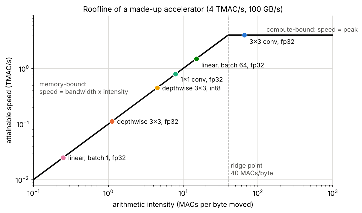
Three lessons recur later. First, the depthwise layer has 64 times fewer MACs than the dense convolution but is estimated to be only about 1.8 times faster, because it is memory-bound (the arithmetic behind the warning in DLCV 01B that MACs are not latency). Second, storing that layer in 8 bits instead of 32 cuts its estimated time by 4 without changing a single MAC: for memory-bound layers, quantization helps by moving fewer bytes. Third, the batch-64 linear layer does 64 times the work of the batch-1 layer in about the same time, because its weights are read once and reused, so throughput at a large batch says little about latency at batch 1.
Measuring honestly
Follow the latency protocol in ML 11 (fixed and reported device, runtime, precision, batch size, resolution and threads; warm-up; percentiles; synchronization on GPUs) and the end-to-end checklist in DLCV 03A. Compression adds three rules of its own:
- Compare against a fair dense baseline: a dense model of the same size, trained with the same budget. Liu et al. found that, for the structured pruning methods they examined, training the pruned architecture from scratch matched or beat fine-tuning the pruned weights [3]; Blalock et al. reviewed 81 pruning papers and found that inconsistent baselines and metrics made most comparisons impossible [4].
- Measure accuracy after export, on the runtime you ship. The exported, quantized, fused graph is a different numerical program from the one you trained.
- Report a trade-off curve, not one point. Accuracy against latency (and memory) for several compression levels shows whether a method moves the whole curve or just picks a different point on it.
Pruning
Plain version. Pruning removes selected weights or channels. Scattered zeros need sparse kernels for speed; removing channels yields smaller dense operations whose latency still needs testing.
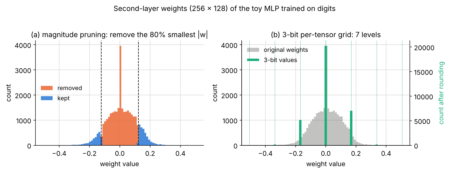
What gets removed
Write the parameters of a network as a vector . Pruning chooses a binary mask and uses instead of , where is elementwise multiplication. The sparsity is the fraction of zeros,
where counts the nonzero entries of the mask. What differs between methods is the granularity of the mask:
- Unstructured (fine-grained): any single weight may be removed. This gives the most freedom in choosing what to remove, but the result is a dense-shaped tensor full of scattered zeros. Li et al. point out that such irregular sparsity does not reduce the cost of convolutional layers much unless sparse convolution libraries are available [5].
- Structured (coarse-grained): whole filters, channels, attention heads or blocks are removed. Removing output channel of a convolution also removes input channel of the next layer, so both tensors shrink and stay dense. Li et al. prune whole filters together with their connecting feature maps for exactly this reason: the result runs with ordinary dense matrix libraries [5].
- Semi-structured: a fixed small pattern that hardware can exploit. NVIDIA’s sparse Tensor Cores support 2:4 sparsity, in which every group of four consecutive weights has at least two zeros; the paper reports twice the math throughput of the dense units for this pattern [6].
Optional: N:M semi-structured sparsity (in the Supplementary notes). How 2:4 weights are stored, the train–prune–retrain workflow, and a NumPy check of how much weight magnitude the pattern costs compared with unstructured pruning.
Which weights: magnitude and other criteria
The simplest and still most common criterion is magnitude: remove the weights with the smallest . It can be applied per layer (remove the same fraction of each layer) or globally (one threshold for the whole network; layers with many small weights then lose more). For structured pruning, the magnitude of a group is used instead: Li et al. rank filters by the sum of absolute weights ( norm) of each filter [5]. Network slimming adds an penalty on the scale factors of the batch-normalization layers during training, which pushes the scales of unimportant channels towards zero, and then removes the channels with the smallest [7]. Many other criteria exist (gradient-based, second-order, data-driven); Hoefler et al. survey them [8].
Structured pruning has one trap that unstructured pruning does not: coupled channels, such as the channels on both sides of a residual addition, which must be removed together. Fang et al.’s DepGraph finds such groups automatically from the computational graph [9].
Optional: Pruning coupled channels (in the Supplementary notes). The dependency rules for residual additions, depthwise layers, concatenations and attention heads, worked through on small examples.
Prune, fine-tune, repeat
Removing weights changes the function, so pruning is followed by training. Han et al. described the standard three-step recipe: train the network to learn which connections are important, prune the unimportant ones, and retrain the remaining weights; on ImageNet they reported reducing AlexNet’s parameters from 61 million to 6.7 million and VGG-16’s from 138 million to 10.3 million without accuracy loss [10]. Their Deep Compression pipeline added quantization and Huffman coding on top of pruning [11].
Pruning is often spread over several smaller steps, each followed by some training, instead of one large cut. Zhu and Gupta’s gradual schedule raises the sparsity from zero to its target during training, quickly at first and more slowly near the end [12]. They also compared large-sparse models with small-dense models of the same memory footprint and found the large-sparse ones consistently more accurate across the architectures they tested [12].
Optional: The gradual pruning schedule (in the Supplementary notes). The cubic sparsity formula with every symbol defined, a worked schedule, and the choices it leaves to you.
Code: unstructured and structured pruning of a small MLP
The snippet trains a 64–256–128–10 MLP on scikit-learn’s digits, then prunes it in two ways: by removing the smallest weights in every layer, and by removing whole hidden units (the smallest norm of incoming weights, in both hidden layers). Each pruned model is fine-tuned for 10 epochs, re-applying the mask after every optimizer step. At the end, the most heavily pruned structured model is sliced into a genuinely smaller dense network.
Code · Python · 56 lines
import copy, warnings
import numpy as np
from sklearn.datasets import load_digits
from sklearn.exceptions import ConvergenceWarning
from sklearn.model_selection import train_test_split
from sklearn.neural_network import MLPClassifier
warnings.filterwarnings("ignore", category=ConvergenceWarning)

X, y = load_digits(return_X_y=True)
Xtr, Xte, ytr, yte = train_test_split(X / 16.0, y, test_size=0.3, random_state=0, stratify=y)
base = MLPClassifier(hidden_layer_sizes=(256, 128), max_iter=300, random_state=0).fit(Xtr, ytr)
print(f"dense: {sum(w.size for w in base.coefs_)} weights, test accuracy {base.score(Xte, yte):.3f}")

def fine_tune(net, masks, epochs=10):
    order_rng = np.random.default_rng(0)
    for _ in range(epochs):
        order = order_rng.permutation(len(Xtr))
        for i in range(0, len(Xtr), 128):
            net.partial_fit(Xtr[order[i:i + 128]], ytr[order[i:i + 128]])   # one Adam step
            for w, m in zip(net.coefs_, masks):
                w *= m                                                     # keep pruned weights at zero

def unstructured_masks(net, sparsity):          # smallest |w| in each layer -> 0
    return [np.abs(w) > np.quantile(np.abs(w), sparsity) for w in net.coefs_]

def structured_masks(net, keep):                # drop hidden units with the smallest L1 norm of incoming weights
    masks = [np.ones_like(w) for w in net.coefs_]
    for l in range(len(net.coefs_) - 1):
        norms = np.abs(net.coefs_[l]).sum(axis=0)
        dead = np.argsort(norms)[: int(round((1 - keep) * norms.size))]
        masks[l][:, dead] = 0                   # incoming weights of the unit ...
        masks[l + 1][dead, :] = 0               # ... and its outgoing weights
    return masks

for name, make, levels in [("remove weights", unstructured_masks, [0.8, 0.9, 0.95]),
                           ("keep units", structured_masks, [0.5, 0.25, 0.125])]:
    for level in levels:
        net = copy.deepcopy(base)
        masks = make(net, level)
        for w, m in zip(net.coefs_, masks):
            w *= m
        before = net.score(Xte, yte)
        fine_tune(net, masks)
        kept = int(sum(m.sum() for m in masks))
        print(f"{name} {level:6.1%}: {kept:5d} weights left, "
              f"accuracy {before:.3f} -> {net.score(Xte, yte):.3f} after fine-tuning")

# The last structured model is a genuinely smaller dense network: slice out the live units.
alive = [masks[l].any(axis=0) for l in range(2)]
small_W = [net.coefs_[0][:, alive[0]], net.coefs_[1][alive[0]][:, alive[1]], net.coefs_[2][alive[1]]]
small_b = [net.intercepts_[0][alive[0]], net.intercepts_[1][alive[1]], net.intercepts_[2]]
h = Xte
for l, (w, b) in enumerate(zip(small_W, small_b)):
    h = h @ w + b if l == 2 else np.maximum(h @ w + b, 0)
print("sliced shapes:", [w.shape for w in small_W],
      "| same predictions:", bool((h.argmax(1) == net.predict(Xte)).all()))
Output (toy results):
Code · 8 lines
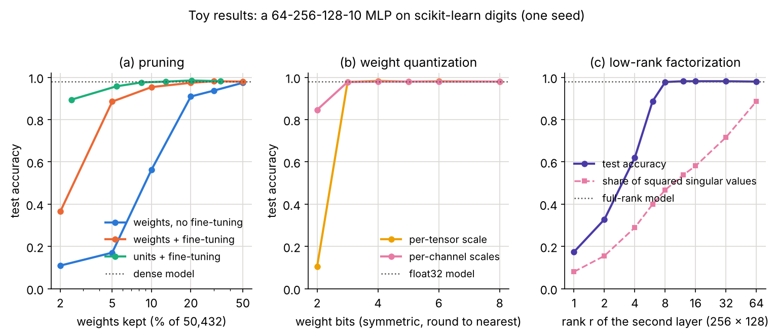
dense: 50432 weights, test accuracy 0.980
remove weights  80.0%: 10087 weights left, accuracy 0.909 -> 0.974 after fine-tuning
remove weights  90.0%:  5044 weights left, accuracy 0.563 -> 0.954 after fine-tuning
remove weights  95.0%:  2523 weights left, accuracy 0.170 -> 0.885 after fine-tuning
keep units  50.0%: 17024 weights left, accuracy 0.887 -> 0.981 after fine-tuning
keep units  25.0%:  6464 weights left, accuracy 0.550 -> 0.980 after fine-tuning
keep units  12.5%:  2720 weights left, accuracy 0.402 -> 0.957 after fine-tuning
sliced shapes: [(64, 32), (32, 16), (16, 10)] | same predictions: True
What to read from it. Fine-tuning does most of the work: removing 90% of the weights drops accuracy to 0.563, and ten epochs bring it back to 0.954. Structured pruning produced a real network of shape 64–32–16–10 that any library runs as ordinary dense matrices. And at about 2,500 remaining weights the small dense network (0.957) beat the large sparse one (0.885), the opposite of Zhu and Gupta’s finding on large models [12]: our network is so over-parameterized for an 8 × 8 digit task that making it narrower costs almost nothing. Do not generalize from this toy in either direction.
The lottery ticket hypothesis
Plain version. If a pruned network can be this small, why not train the small network directly? Frankle and Carbin found that, in their experiments, a randomly reinitialized pruned network trained worse, but the same sparse network reset to its original initial weights trained as well as the full one. They proposed that large networks contain such lucky sparse subnetworks (“winning tickets”) from the start.
The tickets are found by iterative magnitude pruning: train, prune the smallest-magnitude weights, reset the survivors to their initial values, and repeat; on small MNIST and CIFAR-10 networks this consistently found tickets at 10–20% of the original size or less [13]. At ImageNet scale, the weights had to be reset to their values from early in training rather than to initialization [14], and Liu et al. reported that with a well-tuned learning rate the ticket initialization brought no gain over random initialization in their experiments [3]. The practical lesson is modest: the hypothesis is about which sparse networks are trainable, not a cheaper way to compress (finding a ticket costs several full trainings).
Optional: The Lottery Ticket Hypothesis (Frankle and Carbin, ICLR 2019) (in the Paper guides). What the experiments control for, how to read the early-stopping plots, and the limits of the claim.
Quantization
Plain version. A network trained in 32-bit floating point does not need that precision to make good predictions. Quantization stores weights, and often activations, as small integers (8 bits, sometimes 4) together with a few scale factors. That cuts memory by 4 to 8 times and, on hardware with integer arithmetic, also speeds up computation. The difficulty is that a small grid of values has to cover both the many small numbers and the few very large ones.
Uniform affine quantization
The most common scheme, because it permits efficient fixed-point arithmetic [15], maps a real value to an integer and back [16]:
where is the scale (the step between neighbouring representable values), the integer zero point (the integer that represents the real value 0 exactly), the integer range of a -bit format (for example for unsigned 8-bit or for a symmetric signed format), rounding to the nearest integer, clamping into the range, and the dequantized approximation of . For a real range that contains 0, a common choice is
Symmetric quantization fixes and uses a signed range. Exact representation of 0 matters because zero padding and ReLU outputs produce many exact zeros [15]. Two kinds of error arise: rounding error, at most for values inside the range, and clipping error for values outside it. A larger range reduces clipping but makes , and therefore the rounding error, larger [15]. ML 11 has a tested implementation and the error-versus-bits curve.
Why integer kernels can factor out the scales
Plain version. Integers are only useful if the expensive part of a layer, the long sum of products, can run entirely in integers. With one scale per weight row and one per activation tensor, the scales can be pulled out of the sum and applied once at the end.
For one output of a linear layer (a convolution is the same sum over a patch), quantize the weights symmetrically with one scale per output channel, , and the inputs affinely with scale and zero point , . Then
where the sum involves only integers and is accumulated in a 32-bit integer register, and the single product is applied once per output. This is why per-channel scales for weights are cheap (one factor per output channel), while per-channel scales for activations are not: they would sit inside the sum and require rescaling the accumulator for each input channel [15]. It is also why a common choice is symmetric weights and asymmetric activations: an asymmetric weight zero point would add a data-dependent term to every output [15]. Biases are typically kept as 32-bit integers [16].
Code · Python · 24 lines
import numpy as np

rng = np.random.default_rng(0)
W = rng.normal(0, 0.2, size=(16, 256))              # a layer: 16 outputs, 256 inputs
x = rng.normal(0.3, 1.0, size=256)                  # input activations (not centred at 0)

# Weights: symmetric int8, one scale per output channel (zero point 0).
s_w = np.abs(W).max(axis=1) / 127
W_q = np.round(W / s_w[:, None]).astype(np.int8)

# Activations: affine uint8 with a scale and an integer zero point.
lo, hi = min(x.min(), 0.0), x.max()
s_x = (hi - lo) / 255
z_x = int(np.round(-lo / s_x))
x_q = np.clip(np.round(x / s_x) + z_x, 0, 255).astype(np.uint8)
print("activation scale:", round(s_x, 5), "| zero point:", z_x)

# Integer-only inner products, accumulated in int32, then one rescale per output.
acc = W_q.astype(np.int32) @ (x_q.astype(np.int32) - z_x)
y_int = s_w * s_x * acc
y_ref = W @ x
print("max |integer result - float result|:", np.abs(y_int - y_ref).max().round(4))
print("relative error:", (np.linalg.norm(y_int - y_ref) / np.linalg.norm(y_ref)).round(4))
print("largest |accumulator|:", np.abs(acc).max(), "| int16 limit:", 2**15 - 1)
Output:
Code · 4 lines
activation scale: 0.01967 | zero point: 117
max |integer result - float result|: 0.0495
relative error: 0.0083
largest |accumulator|: 83167 | int16 limit: 32767
The integer path reproduces the float result to within about 1%. The accumulator reaches 83,167, far beyond what 16 bits can hold, which is why accelerators keep 32-bit accumulators even when inputs are 8-bit [15]. Before the next layer, the 32-bit result is converted back to 8 bits (“requantized”) with the next layer’s scale.
Optional: Requantization with a fixed-point multiplier (in the Supplementary notes). How Jacob et al. turn the combined real-valued scale into an integer multiply and a bit shift, so that no floating-point operation is left at inference.
Granularity and range setting
Granularity is how many values share one scale: one per tensor, one per output channel, or one per small group of consecutive weights. Finer granularity fits the grid to each group’s own range. Range setting (or calibration) is how is chosen [15]:
- Min-max: the observed minimum and maximum. No clipping, but one outlier stretches the grid for everyone.
- Percentile: ignore a small fraction of the most extreme values.
- MSE: search for the range that minimizes on representative data, trading clipping against rounding.
Weights are known in advance and need no data. Activations depend on the input, so their ranges are estimated by running a small calibration set of unlabeled images through the network; Nagel et al. note that 500 to 1,000 unlabeled images are usually enough [15].
Optional: Choosing the clipping range: min-max, percentile and MSE (in the Supplementary notes). A tested comparison showing that the best rule changes with the bit width: at 8 bits keep the outliers, at 4 bits clip them.
What breaks: outliers, folded batch norm and activations
Plain version. Quantization fails when one shared scale must cover values of very different sizes. The large values force a coarse grid, and the many small values all round to the same few integers.
The classic vision example is MobileNetV2. Nagel et al. showed that the weight ranges of different output channels of one of its depthwise-separable layers differ so much that one set of quantization parameters cannot serve the whole tensor; with batch normalization folded and 8-bit per-tensor quantization, the ImageNet top-1 accuracy of their model fell from 71.72% to 0.12% [17]. Their fix needs no data or training: because for , an output channel of one layer can be scaled down and the matching input channel of the next layer scaled up without changing the function (cross-layer equalization). After replacing ReLU6 by ReLU, which has this property, equalization and bias absorption brought the model to 70.92% at 8 bits [17].
Our toy reproduces the mechanism. We take the trained MLP and rescale one hidden unit by 100 (and the next layer’s weights by 1/100). The float network computes exactly the same function, but its activation and weight ranges now contain one huge channel.
Code · Python · 48 lines
import warnings
import numpy as np
from sklearn.datasets import load_digits
from sklearn.exceptions import ConvergenceWarning
from sklearn.model_selection import train_test_split
from sklearn.neural_network import MLPClassifier
warnings.filterwarnings("ignore", category=ConvergenceWarning)

X, y = load_digits(return_X_y=True)
Xtr, Xte, ytr, yte = train_test_split(X / 16.0, y, test_size=0.3, random_state=0, stratify=y)
net = MLPClassifier(hidden_layer_sizes=(256, 128), max_iter=300, random_state=0).fit(Xtr, ytr)

def q_weight(w, bits, per_channel):     # symmetric: one scale per output unit, or one per tensor
    qmax = 2 ** (bits - 1) - 1
    m = np.abs(w).max(axis=0, keepdims=True) if per_channel else np.abs(w).max()
    return np.clip(np.round(w * qmax / m), -qmax, qmax) * m / qmax

def q_act(a, hi, bits):                 # post-ReLU activations: grid on [0, hi], zero point 0
    s = hi / (2 ** bits - 1)
    return np.clip(np.round(a / s), 0, 2 ** bits - 1) * s

def run(Ws, bs, X, wbits=None, abits=None, his=None, per_channel=True, record=None):
    h = X
    for l, (w, b) in enumerate(zip(Ws, bs)):
        h = h @ (q_weight(w, wbits, per_channel) if wbits else w) + b
        if l < len(Ws) - 1:
            h = np.maximum(h, 0)
            if record is not None:
                record.append(h)
            if abits:
                h = q_act(h, his[l], abits)
    return h

acc = lambda logits: (logits.argmax(1) == yte).mean()
for c in [1, 100]:
    Ws = [w.copy() for w in net.coefs_]
    bs = [b.copy() for b in net.intercepts_]
    Ws[0][:, 0] *= c; bs[0][0] *= c; Ws[1][0, :] /= c   # same function: ReLU(c*t) = c*ReLU(t)
    calib = []
    run(Ws, bs, Xtr[:100], record=calib)                 # 100 training images calibrate the ranges
    minmax = [a.max() for a in calib]
    pct99 = [np.percentile(a, 99) for a in calib]
    print(f"unit 0 scaled by {c}: float {acc(run(Ws, bs, Xte)):.3f} | "
          f"W8A8 {acc(run(Ws, bs, Xte, 8, 8, minmax)):.3f} | "
          f"W8A4 {acc(run(Ws, bs, Xte, 8, 4, minmax)):.3f} | "
          f"W8A4 clipped {acc(run(Ws, bs, Xte, 8, 4, pct99)):.3f} | "
          f"W4 per-tensor {acc(run(Ws, bs, Xte, 4, per_channel=False)):.3f} | "
          f"W4 per-channel {acc(run(Ws, bs, Xte, 4)):.3f}")
Output (toy results; “W8A4” means 8-bit weights and 4-bit activations):
Code · 2 lines
unit 0 scaled by 1: float 0.980 | W8A8 0.980 | W8A4 0.978 | W8A4 clipped 0.978 | W4 per-tensor 0.983 | W4 per-channel 0.980
unit 0 scaled by 100: float 0.980 | W8A8 0.980 | W8A4 0.163 | W8A4 clipped 0.980 | W4 per-tensor 0.102 | W4 per-channel 0.978
The two networks are the same function, yet with one outlier channel, 4-bit min-max activations collapse to 0.163 and 4-bit per-tensor weights to 0.102. Clipping the activation range at the 99th percentile (0.980) and per-unit weight scales (0.978) both fix it. Here clipping happens to cost nothing; when the outlier channel carries real information it does, which is why methods that move or isolate outliers exist.
The same pattern, at larger scale, drives quantization research for Transformers: Dettmers et al. found systematic outlier feature dimensions in large language models and kept them in 16-bit [18], and SmoothQuant moves the difficulty from activations to weights with an equivalent per-channel rescaling, the same family of idea as cross-layer equalization [19].
Post-training quantization and quantization-aware training
Plain version. You can quantize a finished model with a little calibration data (fast, no labels), or you can train the model while it “feels” the rounding, so that it learns weights that survive it (slower, more accurate at low bit widths).
Post-training quantization (PTQ) takes a trained float model and converts it using only a small calibration set. Nagel et al.’s recommended pipeline is: cross-layer equalization, symmetric weight and asymmetric activation quantizers (per-channel weights if the hardware supports it), MSE-based weight ranges, then AdaRound (a learned choice between rounding each weight up or down [20]) if calibration data is available, analytical bias correction otherwise, and finally activation range setting [15].
Quantization-aware training (QAT) inserts “fake quantization” (quantize, then immediately dequantize) into the forward pass and trains as usual. The difficulty is that has zero gradient almost everywhere. The straight-through estimator (STE) [21] treats rounding as the identity in the backward pass. For the symmetric quantizer this gives
so gradients pass unchanged through values inside the range and stop at clipped values [15]. The float “shadow” weights are updated, and the forward pass always uses their quantized version.
When to use which: in the white paper’s experiments PTQ was sufficient for 8-bit weights and activations (within 0.7% of float for every model tested), while lower bit widths, and 4-bit activations in particular, needed QAT; networks with depthwise-separable layers remained the hardest even with QAT [15].
Optional: Beyond round-to-nearest: AdaRound, BRECQ and LSQ (in the Supplementary notes). Three refinements: learning whether to round each weight up or down, reconstructing whole blocks, and learning the scale itself during QAT.
Mixed precision and other number formats
Not all layers are equally sensitive, so mixed-precision quantization gives different layers different bit widths: HAWQ chooses them from second-order (Hessian) information [22], HAQ from latency and energy feedback of a hardware simulator, finding that the best policies differ between edge and cloud accelerators [23]. Integers are not the only option: 8-bit floating-point encodings (E4M3 and E5M2) [24] spend bits on an exponent, which tolerates a wider range of magnitudes at the cost of fewer steps.
Do not confuse this with mixed-precision training (DLCV 01A), which keeps a 32-bit master copy of the weights and computes in 16-bit to speed up training. Mixed-precision quantization is about the deployed model.
Knowledge distillation
Plain version. Train a small student to imitate a large teacher, not only the correct labels. The teacher’s full output (which wrong classes it considers plausible) and its intermediate features carry more information per example than a label does, so the student learns more from the same images.
The response-based loss of Hinton et al., with temperature and the factor, is derived and tested in the DLCV 01 Supplementary notes and summarized in ML 11 [25]; we do not repeat it. In one line: the student minimizes , where and are the student and teacher logits, the label, the softmax, cross-entropy and the weight of the soft term. Hinton et al. show that matching logits, as Ba and Caruana did by regressing them with an L2 loss [26], is the high-temperature limit of this loss [25].
Code: distilling the toy MLP into an 8-unit student
The teacher is the 50,432-weight MLP from the pruning snippet. The student has one hidden layer of 8 units (592 weights) and is trained by full-batch gradient descent, once on labels only and twice with the distillation loss.
Code · Python · 43 lines
import warnings
import numpy as np
from sklearn.datasets import load_digits
from sklearn.exceptions import ConvergenceWarning
from sklearn.model_selection import train_test_split
from sklearn.neural_network import MLPClassifier
warnings.filterwarnings("ignore", category=ConvergenceWarning)

X, y = load_digits(return_X_y=True)
Xtr, Xte, ytr, yte = train_test_split(X / 16.0, y, test_size=0.3, random_state=0, stratify=y)
teacher = MLPClassifier(hidden_layer_sizes=(256, 128), max_iter=300, random_state=0).fit(Xtr, ytr)
h = Xtr
for l, (w, b) in enumerate(zip(teacher.coefs_, teacher.intercepts_)):   # teacher logits
    h = h @ w + b if l == 2 else np.maximum(h @ w + b, 0)
z_teacher = h

def softmax(z, T=1.0):
    e = np.exp((z - z.max(axis=1, keepdims=True)) / T)
    return e / e.sum(axis=1, keepdims=True)

def train_student(T, alpha, hidden=8, steps=500, lr=0.2, seed=0):
    """64 -> 8 -> 10 ReLU network, full-batch gradient descent on the distillation loss."""
    rng = np.random.default_rng(seed)
    W1, b1 = rng.normal(0, np.sqrt(2 / 64), (64, hidden)), np.zeros(hidden)
    W2, b2 = rng.normal(0, np.sqrt(1 / hidden), (hidden, 10)), np.zeros(10)
    Y, p_T = np.eye(10)[ytr], softmax(z_teacher, T)
    for _ in range(steps):
        a = np.maximum(Xtr @ W1 + b1, 0)
        z = a @ W2 + b2
        # gradient of (1-alpha)*CE(y, softmax(z)) + alpha*T^2*CE(p_T, softmax(z/T)) w.r.t. z
        g = ((1 - alpha) * (softmax(z) - Y) + alpha * T * (softmax(z, T) - p_T)) / len(Xtr)
        ga = (g @ W2.T) * (a > 0)
        W2 -= lr * a.T @ g;  b2 -= lr * g.sum(0)
        W1 -= lr * Xtr.T @ ga; b1 -= lr * ga.sum(0)
    return (np.maximum(Xte @ W1 + b1, 0) @ W2 + b2).argmax(1)

print(f"teacher: {sum(w.size for w in teacher.coefs_)} weights, accuracy {teacher.score(Xte, yte):.3f}")
for T in (1, 4):
    print(f"mean top probability of the teacher on training images at T = {T}: "
          f"{softmax(z_teacher, T).max(axis=1).mean():.3f}")
for name, T, alpha in [("labels only", 1, 0.0), ("distill, T = 1", 1, 0.5), ("distill, T = 4", 4, 0.5)]:
    accs = [(train_student(T, alpha, seed=s) == yte).mean() for s in range(5)]
    print(f"student (592 weights), {name:14s}: accuracy {np.mean(accs):.3f} +/- {np.std(accs):.3f} over 5 seeds")
Output (toy results):
Code · 6 lines
teacher: 50432 weights, accuracy 0.980
mean top probability of the teacher on training images at T = 1: 0.998
mean top probability of the teacher on training images at T = 4: 0.787
student (592 weights), labels only   : accuracy 0.936 +/- 0.025 over 5 seeds
student (592 weights), distill, T = 1: accuracy 0.936 +/- 0.025 over 5 seeds
student (592 weights), distill, T = 4: accuracy 0.954 +/- 0.006 over 5 seeds
Distillation at raised the student’s mean accuracy from 0.936 to 0.954 and made it much less dependent on the random seed. At it changed nothing, and the second line says why: on its own training images the teacher is almost certain (mean top probability 0.998), so its soft targets are practically the labels. The temperature is what exposes the teacher’s opinion about the wrong classes. The effect is small and specific to this toy; it is the mechanism, not the number, that transfers.
Feature and attention distillation
The teacher’s intermediate representations can be imitated too. FitNets train a thin, deep student so that one of its middle layers (the “guided” layer), passed through a small learned regressor, predicts a middle layer of the teacher (the “hint” layer); the regressor is needed because the two layers have different widths, and the authors use a convolutional regressor to keep its size manageable [27]. Attention transfer imitates where the teacher’s features are active rather than the features themselves: for a feature map it forms a spatial map
where is channel and an exponent (the paper also studies and a max over channels), and trains the student to match the -normalized maps of the teacher at several depths [28]. Because has no channel dimension, teacher and student widths need not match. Gou et al. organize the field by what is transferred (responses, features, relations between examples or layers) and how (offline from a fixed teacher, online, or self-distillation) [29].
What decides whether distillation helps
- Teacher and student must see the same input. Beyer et al. found that distillation works best when teacher and student receive the identical augmented view of each image (“consistent” teaching), when augmentation is aggressive, and when training is very long (“patient”); inconsistent setups plateaued lower in their experiments [30].
- A better teacher is not always a better teacher. Cho and Hariharan found that larger, more accurate teachers often did not produce better students, attributed this to mismatched capacity, found multi-step distillation through intermediate-size models ineffective, and reported that stopping the teacher’s training early mitigated the problem [31].
- Distillation is a training method, not a compression of an existing model: it needs a training run, data, and a student architecture chosen in advance. DeiT, for example, trains a vision Transformer with an extra distillation token that learns from a convolutional teacher (DLCV 02) [32].
Low-rank factorization
Plain version. A big weight matrix often contains much less information than its size suggests. Writing it as the product of two thin matrices replaces one large layer by two small ones, with far fewer weights and operations.
Any matrix has a singular value decomposition , where () and () have orthonormal columns and is diagonal with the singular values . Keeping the largest gives the best rank- approximation in the Frobenius norm (ML 01A):
where is the first columns of and the chosen rank. The layer becomes two layers with weights instead of , which saves weights and MACs only if . For a convolution with kernel , reshape it to a matrix and factorize: becomes a convolution with output channels and a convolution back to channels. Denton et al. exploited such linear structure in convolutional filters to speed up convolutional layers about twofold on CPU and GPU with accuracy within 1% [33]; Jaderberg et al. built filter bases that are rank-1 in the spatial domain (a followed by a filter) [34]; Zhang et al. extended low-rank acceleration to very deep networks for classification and detection, minimizing the reconstruction error of each layer’s nonlinear responses rather than of its weights [35].
Code · Python · 21 lines
import warnings
import numpy as np
from sklearn.datasets import load_digits
from sklearn.exceptions import ConvergenceWarning
from sklearn.model_selection import train_test_split
from sklearn.neural_network import MLPClassifier
warnings.filterwarnings("ignore", category=ConvergenceWarning)

X, y = load_digits(return_X_y=True)
Xtr, Xte, ytr, yte = train_test_split(X / 16.0, y, test_size=0.3, random_state=0, stratify=y)
net = MLPClassifier(hidden_layer_sizes=(256, 128), max_iter=300, random_state=0).fit(Xtr, ytr)
(W1, W2, W3), (b1, b2, b3) = net.coefs_, net.intercepts_

U, S, Vt = np.linalg.svd(W2, full_matrices=False)       # W2 is 256 x 128
energy = np.cumsum(S**2) / np.sum(S**2)
for r in [4, 8, 16, 32, 128]:
    A, B = U[:, :r] * S[:r], Vt[:r]                     # W2 ~ A @ B: a 256->r and an r->128 layer
    h = np.maximum(np.maximum(Xte @ W1 + b1, 0) @ A @ B + b2, 0)
    acc = ((h @ W3 + b3).argmax(1) == yte).mean()
    print(f"rank {r:3d}: {A.size + B.size:5d} weights instead of {W2.size} "
          f"({energy[r - 1]:.0%} of the squared singular values), accuracy {acc:.3f}")
Output (toy results):
Code · 5 lines
rank   4:  1536 weights instead of 32768 (29% of the squared singular values), accuracy 0.620
rank   8:  3072 weights instead of 32768 (47% of the squared singular values), accuracy 0.978
rank  16:  6144 weights instead of 32768 (58% of the squared singular values), accuracy 0.981
rank  32: 12288 weights instead of 32768 (72% of the squared singular values), accuracy 0.981
rank 128: 49152 weights instead of 32768 (100% of the squared singular values), accuracy 0.980
Rank 8 keeps the accuracy with less than a tenth of the layer’s weights, although it keeps only 47% of the squared singular values. The Frobenius error of the weights is a poor guide to the error of the task: what matters is what the layer does to the inputs it actually sees, which is why Zhang et al. minimize response error instead [35]. The last line shows the break-even rule: at full rank the factorized form has more weights than the original, because . Splitting one layer into two also adds a memory round trip for the intermediate result, so on a memory-bound device the latency saving is smaller than the MAC saving.
The three toys side by side
Designing small from the start
Plain version. Instead of shrinking a big network after training, you can choose an architecture that is small and hardware-friendly from the beginning, either by hand (efficient blocks) or by search. In practice the two approaches are combined: a well-designed small network is then quantized, and sometimes pruned or distilled.
The main hand-designed families are covered elsewhere and only listed here: depthwise-separable convolutions and inverted residuals (MobileNet [36], MobileNetV2 [37]; derivation and cost in DLCV 02 and ML 03), compound scaling of depth, width and resolution (EfficientNet [38]; DLCV 02), and the block-by-block cost arithmetic in DLCV 01B. The roofline view from the start of this chapter is the right lens for all of them: a block is efficient on a device if it does enough arithmetic per byte for that device and has fast kernels there.
Re-parameterization: train rich, deploy plain
Structural re-parameterization trains a block with several parallel linear branches and merges them into one convolution for deployment. RepVGG trains blocks with a convolution, a convolution and an identity branch, each followed by batch normalization, and deploys a plain stack of convolutions and ReLUs [39]. The folding is derived and checked numerically in the DLCV 03A Supplementary notes and, for enhancement networks, in the DLCV 09C Supplementary notes.
Re-parameterization interacts with quantization. The YOLOv6 report states that, because of its heavy use of re-parameterized blocks, earlier PTQ techniques failed to produce good results; in its version 1.0, YOLOv6-S fell from 42.4 to 35.0 COCO val AP under 8-bit PTQ, and to 40.9 when trained with RepOptimizer, which narrowed the activation distribution [40]. The merged kernel adds branches with very different ranges, which is exactly the situation per-tensor quantization handles worst.
Neural architecture search
Plain version. Neural architecture search (NAS) lets an algorithm choose layer types, widths and kernel sizes, scoring candidates by accuracy and, in its hardware-aware form, by measured latency on the target device.
Elsken et al. describe every NAS method by three choices: the search space (which architectures are allowed), the search strategy (how candidates are proposed) and the performance estimation strategy (how a candidate is scored without training it fully) [41]. Three ideas matter for compression:
- Weight sharing makes search affordable. The original reinforcement-learning approach trained each proposed architecture separately [42]; ENAS lets all candidates share the weights of one large graph [43], DARTS relaxes the discrete choice into a continuous one optimized by gradient descent [44], and Once-for-All trains one network from which sub-networks of different depth, width, kernel size and resolution are extracted for different devices without retraining [45].
- Search for measured latency, not FLOPs. MnasNet puts latency measured on real phones into the objective [46]; ProxylessNAS searches directly on the target task and hardware [47]; FBNet’s differentiable search is motivated by the same observation that FLOPs do not always reflect latency [48].
- Keep a random baseline. Li and Talwalkar found random search with early stopping at least as good as ENAS on the two benchmarks they used [49].
Deployment: from a small model to a fast one
Plain version. A compressed model becomes fast only after a compiler or runtime turns it into a few large, fused operations with kernels that support its number format and sparsity pattern. Speed claims from papers often assume support that your device does not have.
Operator fusion and batch-norm folding
Each separate operation reads its input from memory and writes its output back. Operator fusion merges consecutive operations (convolution, bias, batch normalization, activation) into one kernel so that intermediate results stay in fast on-chip memory; from the roofline viewpoint, it raises arithmetic intensity by removing memory round trips. The most common fusion is batch-norm folding: at inference, batch normalization [50] with learned scale , shift , running mean and variance is an affine map per output channel , so it can be absorbed into the preceding convolution,
where and are the kernel and bias of output channel and a small constant. A tested NumPy version is in the DLCV 03A Supplementary notes. For compression, notice the factor : it differs from channel to channel, so folding can spread the per-channel weight ranges apart, which is one reason MobileNetV2 was hard to quantize per tensor [17]. On device, batch normalization is folded before quantization, so the folded weights are what the integer kernel sees, and QAT has to simulate the folding correctly [15].
Integer kernels and runtime support
Quantization speeds up inference only if the runtime has integer (or low-precision) kernels for every operation in the graph. ML 11 shows a weight-only int8 model that is four times smaller but slower, because it converts weights back to float on every call. In a real deployment, check: does the target support per-channel weight scales (not all hardware does [15]); which operators fall back to float (each fallback adds a dequantize and a quantize); and whether the runtime keeps the graph in integers between layers. The export and runtime tools themselves (ONNX, ONNX Runtime, TensorRT, torch.export) are described in ML 11.
Why paper speed-ups shrink on devices
- FLOPs are not the bottleneck. A method that removes 90% of the MACs of memory-bound layers barely changes their time (Figure 1).
- Sparsity needs kernels. Unstructured sparsity speeds up only with sparse kernels for that pattern on that device [5], [8]; 2:4 sparsity has dedicated hardware on some GPUs [6]; structured pruning needs nothing special.
- Batch size. Throughput at a large batch is not latency at batch 1 (the linear-layer example above).
- The rest of the pipeline. Pre-processing, post-processing such as NMS (DLCV 03A), resizing and data transfer do not shrink when the network does.
- Unsupported operators. A single operator without a low-precision kernel can force conversions that cost more than they save.
Compressing vision models: what is sensitive
Plain version. Different parts of a vision model react very differently to compression. Layers with few weights per channel, outputs that must be numerically precise (box coordinates, pixel values), and activations whose range changes from image to image are the usual weak points.
Classification backbones
Networks built from depthwise-separable layers are the hardest common backbones to quantize. With 4-bit weights and 8-bit activations, per-tensor PTQ cost MobileNetV2 and EfficientNet-lite about 2.5 and 4.2 points of ImageNet top-1 in Nagel et al.’s experiments, which they attribute likely to the depthwise-separable convolutions; per-channel scales recovered 2.8 points for EfficientNet-lite [15]. Layers whose weight ranges differ strongly across channels are the first candidates for per-channel scales or higher precision, and a per-layer sensitivity test (quantize one layer at a time and measure the drop, as in Exercise 5) finds the others quickly.
Detectors
Detectors predict continuous box coordinates and scores, and both suffer from coarse grids. In the white paper, EfficientDet-D1 reached 40.08 COCO mAP in float and 38.29 with 8-bit PTQ, but only 0.31 with 4-bit per-tensor weights (35.08 per-channel); QAT brought the 4-bit-weight results to 35.34 and 36.75 [15]. Re-parameterized detectors such as YOLOv6 need quantization-friendly training (above) [40]. Because strict-IoU accuracy is what coarse box coordinates hurt first, check AP at high IoU thresholds after quantizing, not only AP at IoU 0.5 (DLCV 03A).
Distillation also needs care for detectors. Wang et al. found that applying ordinary distillation to a detector gave only minor gains, and instead had the student imitate the teacher’s features at locations near objects, estimated from the anchors; this improved students on KITTI, Pascal VOC and COCO in their experiments [51].
Dense prediction and restoration
For super-resolution, denoising and enhancement the output is an image, and every quantization error can become visible. Two properties make these networks harder than classifiers. First, many restoration networks remove batch normalization; Li et al. found that this leaves activations with a much larger dynamic range, which breaks quantization schemes that assume normalized activations, and proposed learning a max scale per layer (PAMS) [52]. Second, Hong et al. observed that in super-resolution networks each channel has a different activation distribution, which also changes with the input image, and proposed channel-wise distribution-aware quantization (DAQ) [53]. So calibrate on images like the deployment content (dark scenes for a low-light model), evaluate at full resolution with the metrics of DLCV 09, and inspect smooth gradients, where banding appears first. The NTIRE efficient super-resolution challenges rank runtime, FLOPs and parameters in separate tracks under a fixed PSNR threshold [54] (DLCV 09A); DLCV 09C covers efficient enhancement networks.
Vision Transformers and diffusion models
In vision Transformers, the activations after softmax and GELU are far from Gaussian, which PTQ4ViT handles with two ranges per such tensor [55]; Liu et al. add a ranking loss so that quantized attention keeps the order of the attention scores [56]. Diffusion models add a time dimension: the same denoising network runs at many noise levels, and its activation distributions change with the time step. Q-Diffusion identifies this, together with bimodal activations in shortcut layers, as the key difficulty and uses time-step-aware calibration [57]; PTQ4DM studies the same multi-time-step calibration problem [58]. Large segmentation foundation models are compressed by distillation: MobileSAM distills the large image encoder of the Segment Anything Model [59] into a small one (“decoupled distillation”) [60], and EfficientSAM pre-trains small encoders to reconstruct SAM’s features [61].
Modern view
What the surveys say
- General compression. Cheng et al. divide the field into four categories: parameter pruning and quantization, low-rank factorization, transferred/compact convolutional filters, and knowledge distillation, and discuss each category’s advantages and drawbacks [62]. Menghani organizes efficient deep learning into five areas: compression techniques, learning techniques (such as distillation), automation (hyper-parameter optimization and architecture search), efficient architectures, and infrastructure (software and hardware), and adds a practitioner’s guide [63].
- Quantization. Gholami et al. survey quantization from the basics (uniform and non-uniform quantizers, range calibration, granularity, fine-tuning) to advanced topics (integer-only inference, mixed precision, hardware-aware and distillation-assisted quantization, extreme low-bit quantization) [64]; Nagel et al.’s white paper is the practical companion, with tested PTQ and QAT pipelines and a debugging workflow [15].
- Pruning and sparsity. Hoefler et al. distill more than 300 papers on sparsity for inference and training, including how to obtain real speed-ups on hardware [8]. Cheng, Zhang and Shi organize pruning by universal or specific speed-up, when to prune, how to prune, and fusion with other compression techniques, and cover pruning of large language and multimodal models [65]. Blalock et al. remain the cautionary reference on how pruning results are reported [4].
- Distillation. Gou et al. categorize distillation by knowledge type, training scheme, teacher–student architecture and algorithm [29]; Wang and Yoon focus on vision and on why distillation works [66].
- Architecture search. Elsken et al. provide the three-dimension taxonomy used above [41]; White et al., writing after more than 1,000 NAS papers, give a taxonomy of search spaces, algorithms and speed-up techniques together with benchmarks and best practices [67].
Optional: A White Paper on Neural Network Quantization (Nagel et al., 2021) (in the Paper guides). How its pipelines are built and how to read its PTQ and QAT tables.
The state of the art, 2023–2026
- Low-bit weights for very large models. Weight-only quantization to 3–4 bits with error-compensating rounding (GPTQ [68]) or activation-aware protection of salient channels (AWQ [69]) became standard for large Transformers; ML 11 introduces both. SmoothQuant made 8-bit weights and activations practical for language models by migrating outliers from activations to weights [19].
- Generative vision models at 4 bits. After Q-Diffusion [57], SVDQuant quantizes both weights and activations of large diffusion models to 4 bits by moving activation outliers into the weights and absorbing the weight outliers with a small high-precision low-rank branch, fused into the low-bit kernel to avoid extra memory traffic; it combines two techniques of this chapter, low-rank factorization and quantization [70].
- Floating-point 8-bit formats (E4M3, E5M2) as an alternative to int8 for both training and inference [24].
- Distilled foundation models. Small students of large vision foundation models, such as MobileSAM and EfficientSAM for segmentation [60], [61], and the distilled DINOv2 backbones discussed in DLCV 02.
- Structural pruning for any graph. DepGraph-style dependency analysis makes channel pruning applicable to CNNs, Transformers and other architectures with one method [9].
- Challenge-driven efficient restoration, where runtime, FLOPs and parameters are scored separately [54].
Open problems
- Predicting device speed. FLOPs and parameters still dominate papers, but only measured latency on the target matters, and it depends on kernels, memory and batch size [1].
- Fair comparisons. Baselines of equal size and training budget, multiple seeds and full trade-off curves are still often missing [4], [3].
- Low-bit activations. 4-bit weights are increasingly routine; 4-bit activations, especially in networks with depthwise layers, attention and time-varying distributions, still cost accuracy [15], [57].
- What compression changes beyond accuracy. Average accuracy can hide changes on rare classes, shifted inputs or calibration; measuring these after compression is still not standard practice.
- Compression of restoration and generative models, where the error is visible in the output and no single metric captures it.
Key takeaways
- Define the actual deployment budget and measure end-to-end cost on the target device.
- Fewer MACs may not help memory-bound layers; inspect bytes moved and available kernels.
- Unstructured pruning needs sparse support for speed; structured pruning creates smaller dense layers but still needs measurement.
- Start with PTQ, inspect calibration and outliers, and use QAT when the required precision loses too much accuracy.
- Distillation depends on teacher information, matched input views and training; a larger teacher is not automatically better.
- Validate compressed models after export, including sensitive outputs; compare against equally well-trained small dense models.
Exercises
- Roofline arithmetic. On the made-up accelerator of the first snippet (4 TMAC/s, 100 GB/s), estimate the time of a convolution with 128 input and 128 output channels on a map in 16-bit precision. Is it compute- or memory-bound? Then find the smallest batch size at which a fp32 linear layer becomes compute-bound.
Hint
The convolution does M MACs and moves values, or about 0.70 MB at 2 bytes each, so its intensity is about 166 MACs per byte: compute-bound, about 28.9 µs. For the linear layer at batch , intensity is ; setting it to 40 gives . Adapt the layer function from the snippet to check.
- Large-sparse or small-dense? In the pruning snippet, the narrow dense network beat the sparse one at about 2,500 weights, unlike Zhu and Gupta’s results on large models. Design an experiment on the toy that would make the comparison fairer (think about what each model was allowed to train for and how it was initialized), and predict how the result would change if the original network were already narrow, for example 64–32–16–10.
Hint
Give both models the same total number of optimizer steps, tune their learning rates separately, and add a third model: the narrow architecture trained from scratch (the baseline that Liu et al. argue for). A network that is already narrow has little redundancy to remove, so structured pruning should lose accuracy faster, and the unstructured model, which can keep important weights anywhere, may then win.
- Quantize by hand. Quantize the values to 4-bit unsigned integers with the affine scheme and a min-max range. Compute , , every and every . Why is the error for not zero even though it is the end of the range, and could it be larger than ?
Hint
and , so and . Rounding to an integer shifts the whole grid so that 0 is exact; the grid then spans instead of , so neither end value lies on a grid point (both errors are about 0.053, below ). A value above or below would be clipped, and its error could exceed .
- Temperature and weight in distillation. Rerun the distillation snippet with and . Which settings help the 8-unit student, and why might a very high temperature help less than a moderate one? Use the gradient of the soft term, , in your answer.
Hint
One run gave 0.948 and 0.953 for ( and ), but 0.937 and 0.916 for , against 0.936 with labels only. At a very high temperature the soft targets approach a uniform distribution and say less about the correct class, and with the label term has little weight left; the factor also changes the effective step size, so the learning rate interacts with . Compare differences with the spread over seeds before drawing conclusions.
- Per-layer sensitivity. Using the functions
q_weightandrunfrom the outlier snippet, quantize the weights of one layer at a time to 2 bits (per channel) while keeping the others in float, and rank the three layers by the accuracy drop. Then quantize only the most robust two layers to 2 bits and keep the most sensitive one at 8 bits. What weight memory does this mixed-precision model need compared with all-8-bit?
Hint
Pass a list of quantized and unquantized weight matrices to run instead of using its wbits argument. The layers have , and weights; memory is bytes plus one scale per output unit. This is the idea behind sensitivity-based mixed precision such as HAWQ, with measured accuracy instead of Hessian information.
References
- M. Dehghani, A. Arnab, L. Beyer, A. Vaswani and Y. Tay, “The efficiency misnomer,” ICLR, 2022. arXiv
- S. Williams, A. Waterman and D. Patterson, “Roofline: an insightful visual performance model for multicore architectures,” Communications of the ACM, vol. 52, no. 4, pp. 65–76, 2009. doi
- Z. Liu, M. Sun, T. Zhou, G. Huang and T. Darrell, “Rethinking the value of network pruning,” ICLR, 2019. arXiv
- D. Blalock, J. J. Gonzalez Ortiz, J. Frankle and J. Guttag, “What is the state of neural network pruning?,” MLSys, 2020. arXiv
- H. Li, A. Kadav, I. Durdanovic, H. Samet and H. P. Graf, “Pruning filters for efficient ConvNets,” ICLR, 2017. arXiv
- A. Mishra, J. Albericio Latorre, J. Pool, D. Stosic, D. Stosic, G. Venkatesh, C. Yu and P. Micikevicius, “Accelerating sparse deep neural networks,” arXiv:2104.08378, 2021. arXiv
- Z. Liu, J. Li, Z. Shen, G. Huang, S. Yan and C. Zhang, “Learning efficient convolutional networks through network slimming,” ICCV, 2017. arXiv
- T. Hoefler, D. Alistarh, T. Ben-Nun, N. Dryden and A. Peste, “Sparsity in deep learning: pruning and growth for efficient inference and training in neural networks,” Journal of Machine Learning Research, vol. 22, no. 241, pp. 1–124, 2021. paper
- G. Fang, X. Ma, M. Song, M. B. Mi and X. Wang, “DepGraph: towards any structural pruning,” CVPR, 2023. doi arXiv
- S. Han, J. Pool, J. Tran and W. J. Dally, “Learning both weights and connections for efficient neural networks,” NeurIPS (NIPS), 2015. arXiv
- S. Han, H. Mao and W. J. Dally, “Deep compression: compressing deep neural networks with pruning, trained quantization and Huffman coding,” ICLR, 2016. arXiv
- M. Zhu and S. Gupta, “To prune, or not to prune: exploring the efficacy of pruning for model compression,” arXiv:1710.01878, 2017. arXiv
- J. Frankle and M. Carbin, “The lottery ticket hypothesis: finding sparse, trainable neural networks,” ICLR, 2019. arXiv
- J. Frankle, G. K. Dziugaite, D. M. Roy and M. Carbin, “Linear mode connectivity and the lottery ticket hypothesis,” ICML, 2020. arXiv
- M. Nagel, M. Fournarakis, R. A. Amjad, Y. Bondarenko, M. van Baalen and T. Blankevoort, “A white paper on neural network quantization,” arXiv:2106.08295, 2021. arXiv
- B. Jacob, S. Kligys, B. Chen, M. Zhu, M. Tang, A. Howard, H. Adam and D. Kalenichenko, “Quantization and training of neural networks for efficient integer-arithmetic-only inference,” CVPR, 2018. doi arXiv
- M. Nagel, M. van Baalen, T. Blankevoort and M. Welling, “Data-free quantization through weight equalization and bias correction,” ICCV, 2019. arXiv
- T. Dettmers, M. Lewis, Y. Belkada and L. Zettlemoyer, “LLM.int8(): 8-bit matrix multiplication for transformers at scale,” NeurIPS, 2022. arXiv
- G. Xiao, J. Lin, M. Seznec, H. Wu, J. Demouth and S. Han, “SmoothQuant: accurate and efficient post-training quantization for large language models,” ICML, 2023. arXiv
- M. Nagel, R. A. Amjad, M. van Baalen, C. Louizos and T. Blankevoort, “Up or down? Adaptive rounding for post-training quantization,” ICML, 2020. arXiv
- Y. Bengio, N. Léonard and A. Courville, “Estimating or propagating gradients through stochastic neurons for conditional computation,” arXiv:1308.3432, 2013. arXiv
- Z. Dong, Z. Yao, A. Gholami, M. W. Mahoney and K. Keutzer, “HAWQ: Hessian aware quantization of neural networks with mixed-precision,” ICCV, 2019. arXiv
- K. Wang, Z. Liu, Y. Lin, J. Lin and S. Han, “HAQ: hardware-aware automated quantization with mixed precision,” CVPR, 2019. arXiv
- P. Micikevicius et al., “FP8 formats for deep learning,” arXiv:2209.05433, 2022. arXiv
- G. Hinton, O. Vinyals and J. Dean, “Distilling the knowledge in a neural network,” NIPS Deep Learning Workshop, 2014; arXiv:1503.02531. arXiv
- L. J. Ba and R. Caruana, “Do deep nets really need to be deep?,” NeurIPS (NIPS), 2014. arXiv
- A. Romero, N. Ballas, S. E. Kahou, A. Chassang, C. Gatta and Y. Bengio, “FitNets: hints for thin deep nets,” ICLR, 2015. arXiv
- S. Zagoruyko and N. Komodakis, “Paying more attention to attention: improving the performance of convolutional neural networks via attention transfer,” ICLR, 2017. arXiv
- J. Gou, B. Yu, S. J. Maybank and D. Tao, “Knowledge distillation: a survey,” International Journal of Computer Vision, vol. 129, no. 6, pp. 1789–1819, 2021. doi
- L. Beyer, X. Zhai, A. Royer, L. Markeeva, R. Anil and A. Kolesnikov, “Knowledge distillation: a good teacher is patient and consistent,” CVPR, 2022. arXiv
- J. H. Cho and B. Hariharan, “On the efficacy of knowledge distillation,” ICCV, 2019. arXiv
- H. Touvron, M. Cord, M. Douze, F. Massa, A. Sablayrolles and H. Jégou, “Training data-efficient image transformers & distillation through attention,” ICML, 2021. arXiv
- R. Denton, W. Zaremba, J. Bruna, Y. LeCun and R. Fergus, “Exploiting linear structure within convolutional networks for efficient evaluation,” NeurIPS (NIPS), 2014. arXiv
- M. Jaderberg, A. Vedaldi and A. Zisserman, “Speeding up convolutional neural networks with low rank expansions,” BMVC, 2014. arXiv
- X. Zhang, J. Zou, K. He and J. Sun, “Accelerating very deep convolutional networks for classification and detection,” IEEE Transactions on Pattern Analysis and Machine Intelligence, vol. 38, no. 10, pp. 1943–1955, 2016. doi arXiv
- A. G. Howard, M. Zhu, B. Chen, D. Kalenichenko, W. Wang, T. Weyand, M. Andreetto and H. Adam, “MobileNets: efficient convolutional neural networks for mobile vision applications,” arXiv:1704.04861, 2017. arXiv
- M. Sandler, A. Howard, M. Zhu, A. Zhmoginov and L.-C. Chen, “MobileNetV2: inverted residuals and linear bottlenecks,” CVPR, 2018. arXiv
- M. Tan and Q. V. Le, “EfficientNet: rethinking model scaling for convolutional neural networks,” ICML, 2019. arXiv
- X. Ding, X. Zhang, N. Ma, J. Han, G. Ding and J. Sun, “RepVGG: making VGG-style ConvNets great again,” CVPR, 2021. arXiv
- C. Li et al., “YOLOv6: a single-stage object detection framework for industrial applications,” arXiv:2209.02976, 2022. arXiv
- T. Elsken, J. H. Metzen and F. Hutter, “Neural architecture search: a survey,” Journal of Machine Learning Research, vol. 20, pp. 1–21, 2019. arXiv
- B. Zoph and Q. V. Le, “Neural architecture search with reinforcement learning,” ICLR, 2017. arXiv
- H. Pham, M. Y. Guan, B. Zoph, Q. V. Le and J. Dean, “Efficient neural architecture search via parameter sharing,” ICML, 2018. arXiv
- H. Liu, K. Simonyan and Y. Yang, “DARTS: differentiable architecture search,” ICLR, 2019. arXiv
- H. Cai, C. Gan, T. Wang, Z. Zhang and S. Han, “Once-for-all: train one network and specialize it for efficient deployment,” ICLR, 2020. arXiv
- M. Tan, B. Chen, R. Pang, V. Vasudevan, M. Sandler, A. Howard and Q. V. Le, “MnasNet: platform-aware neural architecture search for mobile,” CVPR, 2019. arXiv
- H. Cai, L. Zhu and S. Han, “ProxylessNAS: direct neural architecture search on target task and hardware,” ICLR, 2019. arXiv
- B. Wu, X. Dai, P. Zhang, Y. Wang, F. Sun, Y. Wu, Y. Tian, P. Vajda, Y. Jia and K. Keutzer, “FBNet: hardware-aware efficient ConvNet design via differentiable neural architecture search,” CVPR, 2019. doi arXiv
- L. Li and A. Talwalkar, “Random search and reproducibility for neural architecture search,” UAI, 2019. arXiv
- S. Ioffe and C. Szegedy, “Batch normalization: accelerating deep network training by reducing internal covariate shift,” ICML, 2015. arXiv
- T. Wang, L. Yuan, X. Zhang and J. Feng, “Distilling object detectors with fine-grained feature imitation,” CVPR, 2019. arXiv
- H. Li, C. Yan, S. Lin, X. Zheng, Y. Li, B. Zhang, F. Yang and R. Ji, “PAMS: quantized super-resolution via parameterized max scale,” ECCV, 2020. arXiv
- C. Hong, H. Kim, S. Baik, J. Oh and K. M. Lee, “DAQ: channel-wise distribution-aware quantization for deep image super-resolution networks,” WACV, 2022. arXiv
- B. Ren, Y. Li, N. Mehta, R. Timofte et al., “The ninth NTIRE 2024 efficient super-resolution challenge report,” CVPR Workshops, 2024. doi arXiv
- Z. Yuan, C. Xue, Y. Chen, Q. Wu and G. Sun, “PTQ4ViT: post-training quantization for vision transformers with twin uniform quantization,” ECCV, 2022. doi arXiv
- Z. Liu, Y. Wang, K. Han, S. Ma and W. Gao, “Post-training quantization for vision transformer,” NeurIPS, 2021. arXiv
- X. Li, Y. Liu, L. Lian, H. Yang, Z. Dong, D. Kang, S. Zhang and K. Keutzer, “Q-Diffusion: quantizing diffusion models,” ICCV, 2023. doi arXiv
- Y. Shang, Z. Yuan, B. Xie, B. Wu and Y. Yan, “Post-training quantization on diffusion models,” CVPR, 2023. arXiv
- A. Kirillov et al., “Segment anything,” ICCV, 2023. doi arXiv
- C. Zhang, D. Han, Y. Qiao, J. U. Kim, S.-H. Bae, S. Lee and C. S. Hong, “Faster segment anything: towards lightweight SAM for mobile applications,” arXiv:2306.14289, 2023. arXiv
- Y. Xiong et al., “EfficientSAM: leveraged masked image pretraining for efficient segment anything,” CVPR, 2024. doi arXiv
- Y. Cheng, D. Wang, P. Zhou and T. Zhang, “Model compression and acceleration for deep neural networks: the principles, progress, and challenges,” IEEE Signal Processing Magazine, vol. 35, no. 1, pp. 126–136, 2018. doi arXiv
- G. Menghani, “Efficient deep learning: a survey on making deep learning models smaller, faster, and better,” ACM Computing Surveys, vol. 55, no. 12, pp. 1–37, 2023. doi arXiv
- A. Gholami, S. Kim, Z. Dong, Z. Yao, M. W. Mahoney and K. Keutzer, “A survey of quantization methods for efficient neural network inference,” book chapter in Low-Power Computer Vision; arXiv:2103.13630, 2021. arXiv
- H. Cheng, M. Zhang and J. Q. Shi, “A survey on deep neural network pruning: taxonomy, comparison, analysis, and recommendations,” IEEE Transactions on Pattern Analysis and Machine Intelligence, vol. 46, no. 12, pp. 10558–10578, 2024. doi arXiv
- L. Wang and K.-J. Yoon, “Knowledge distillation and student-teacher learning for visual intelligence: a review and new outlooks,” IEEE Transactions on Pattern Analysis and Machine Intelligence, vol. 44, no. 6, pp. 3048–3068, 2022. doi arXiv
- C. White, M. Safari, R. Sukthanker, B. Ru, T. Elsken, A. Zela, D. Dey and F. Hutter, “Neural architecture search: insights from 1000 papers,” arXiv:2301.08727, 2023. arXiv
- E. Frantar, S. Ashkboos, T. Hoefler and D. Alistarh, “GPTQ: accurate post-training quantization for generative pre-trained transformers,” ICLR, 2023. arXiv
- J. Lin, J. Tang, H. Tang, S. Yang, W.-M. Chen, W.-C. Wang, G. Xiao, X. Dang, C. Gan and S. Han, “AWQ: activation-aware weight quantization for LLM compression and acceleration,” MLSys, 2024. arXiv
- M. Li, Y. Lin, Z. Zhang, T. Cai, X. Li, J. Guo, E. Xie, C. Meng, J.-Y. Zhu and S. Han, “SVDQuant: absorbing outliers by low-rank components for 4-bit diffusion models,” ICLR, 2025. arXiv
- Y. Li, R. Gong, X. Tan, Y. Yang, P. Hu, Q. Zhang, F. Yu, W. Wang and S. Gu, “BRECQ: pushing the limit of post-training quantization by block reconstruction,” ICLR, 2021. arXiv
- S. K. Esser, J. L. McKinstry, D. Bablani, R. Appuswamy and D. S. Modha, “Learned step size quantization,” ICLR, 2020. arXiv
Check your understanding
This tutorial has 5 exercises. Can you solve them without opening the hints?
Go to the exercises ↑Next DLCV 02 · Deep Image Classification · 45 min