DLCV 08 · Video Understanding and Action Recognition
Needs: DLCV 02 · Deep Image Classification
Navigate: this page and this track: Navigate: this page and this track
On this page
- What you’ll learn1 min
- The big picture2 min
- Video understanding tasks2 min
- Why video is hard4 min
- How to add time to an image network12 min
- Learning video representations without labels2 min
- Video and language, briefly1 min
- Localizing actions in time and space4 min
- Training and evaluating video classifiers3 min
- Failure modes1 min
- Modern view3 min
- Key takeaways1 min
- Exercises3 min
- Supplementary notes
- Paper guides
- References
Deep Learning for Computer Vision
What you’ll learn
- Match video tasks to clip, interval, person-level or language outputs.
- Distinguish temporal reasoning from appearance shortcuts.
- Compare optical-flow streams, temporal convolutions, sampling and attention.
- Understand masked video pretraining and video–language transfer.
- Control frames, views, resolution and pretraining when evaluating performance and cost.
The big picture
An image classifier looks at one picture and names what is in it. A video model must also understand what happens: who does what, in which order, for how long. The extra input is a time axis, and with it come two problems that images do not have. First, time is expensive: a 10-second clip at 30 frames per second is 300 images. Second, time is easy to ignore: a network can often guess “playing tennis” from the court alone, without ever looking at the swing.
Video understanding matters because most visual data is video: phone recordings, surveillance and traffic cameras, sports broadcasts, robots, cars and medical procedures. Recognizing actions is a building block for searching video archives, analyzing sports, monitoring safety, assisting people at home and controlling robots. The field also produced ideas that spread to the rest of deep learning, such as inflating a pretrained 2D network into 3D, factorizing space and time, and masked pretraining at very high masking ratios.
This tutorial assumes image classification, its training and its evaluation from DLCV 02. It reuses detection metrics from DLCV 03 and attention from ML 05. Five surveys frame the field: Zhu et al. on deep action recognition [1], Kong and Fu on recognition and prediction [2], Selva et al. on video transformers [3], Madan et al. on video foundation models [4] and Tang et al. on video understanding with large language models [5]. We return to them in the Modern view.
Related chapters. Following objects over time is DLCV 07 · Object Tracking; body keypoints, which skeleton-based recognition uses as input, are DLCV 05; optical flow is estimated in DLCV 11A; generating video with spatiotemporal attention and video autoencoders is DLCV 12A; and predicting the future of a scene for planning is DLCV 13 · World Models.
Video understanding tasks
Plain version. Video outputs may be a clip label, action intervals, person-level detections or a language answer. Define the required output before choosing a model.
Precise version. A video is a tensor , where is the number of frames, the frame size and 3 the color channels. A model rarely sees all of . It sees a clip of sampled frames, resized and cropped to . Figure 1 shows the four task families.
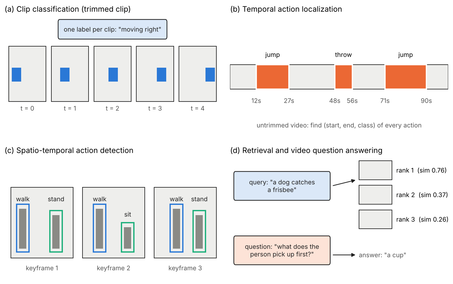
- Clip (action) classification. Given a trimmed clip that contains one action, predict its class . Trained with cross-entropy and evaluated with top-1 and top-5 accuracy, exactly as in DLCV 02. Some datasets are multi-label (several actions at once) and are evaluated with mean average precision (mAP) over classes.
- Temporal action localization (also called temporal action detection). Given an untrimmed video, output a set of segments with start time , end time , class and confidence . It is object detection along one dimension, and it is evaluated with mAP at several temporal IoU thresholds.
- Spatio-temporal action detection. Find who does what, where and when: a person box in each annotated keyframe, with one or more action labels per box. It is evaluated with frame-level mAP at a box-IoU threshold.
- Video–language tasks. Text-to-video retrieval ranks a collection of videos by their similarity to a sentence, evaluated by Recall@ (the fraction of queries whose correct video is among the top ). Video question answering produces a short answer, often chosen from multiple choices and scored by accuracy.
Neighboring problems are covered elsewhere. Linking the same object across frames is tracking (DLCV 07). Predicting what happens next is action anticipation or world modeling (DLCV 13). Labeling every pixel of every frame is video segmentation.
Why video is hard
Plain version. Three things make video harder than images: the label often depends on order and motion, the datasets let models skip that work, and the input is huge.
Time matters, but the data does not always force you to use it
Some actions can only be told apart by their motion: “opening a door” versus “closing a door”, “pushing something left” versus “pushing something right”, “sitting down” versus “standing up”. A single frame of these is ambiguous. Many other actions are recognizable from one frame because of the scene and the objects: a swimming pool, a horse, a guitar. Datasets collected from the web contain many actions of the second kind.
This was visible early. Karpathy et al. trained CNNs on a dataset of 1 million YouTube videos in 487 sports classes and compared several ways of fusing information over time; their best spatio-temporal network improved only modestly over a single-frame model [6]. Later studies measured the problem directly. Li et al. defined the representation bias of a dataset and showed that common action datasets are biased toward static cues (objects, scenes and people); they also built Diving48, a dataset of competitive diving with 48 fine-grained dive classes, to reduce that bias [7]. Sevilla-Lara et al. asked people to recognize actions from videos whose frames had been shuffled, and kept only the classes that became unrecognizable; this “temporal” subset is where a model’s ability to use time actually shows [8]. Something-Something was built to capture detailed physical aspects of actions rather than high-level concepts: its 174 classes are caption templates such as “pushing something from left to right” [9], which the VideoMAE authors describe as motion-centric [10].
The general phenomenon, a network solving the training task with the easiest cue available, is the shortcut learning of DLCV 02. In video the easiest cue is usually the scene.
A dataset where one frame says nothing
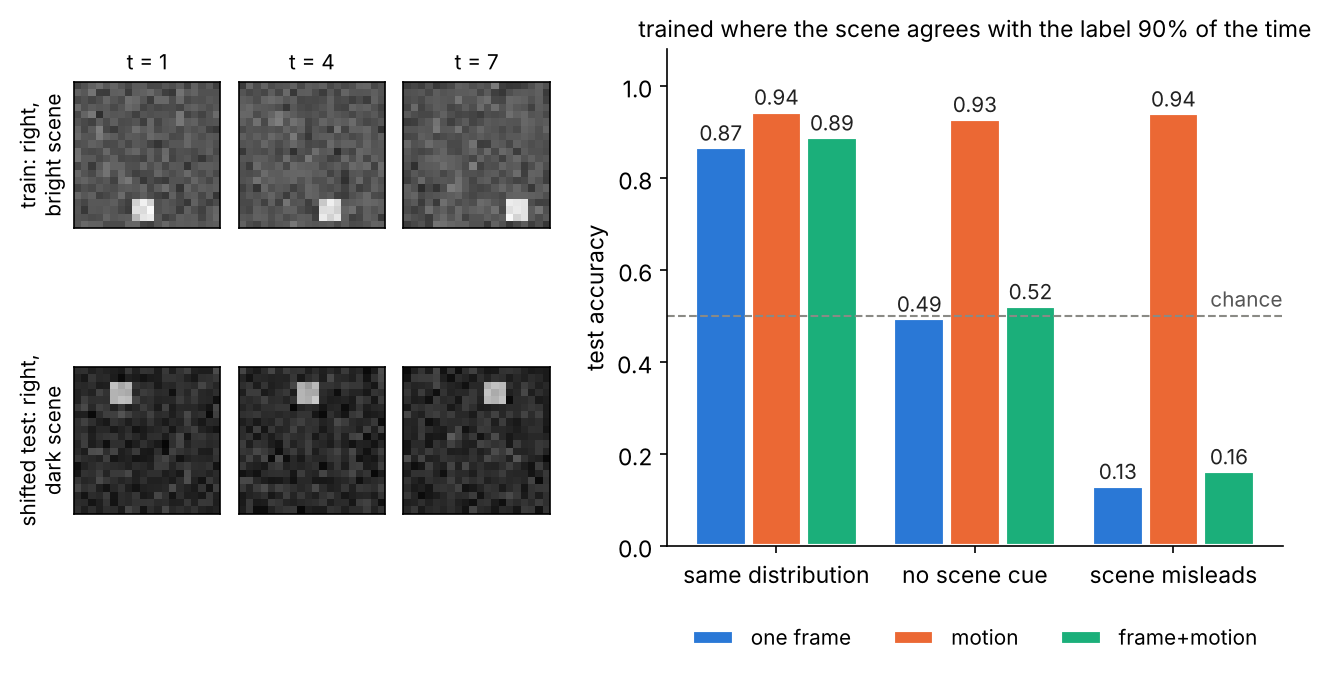
The code below makes this concrete with synthetic clips. A small square moves left or right; the label is the direction. The square’s position in the middle frame has the same distribution for both labels, so the middle frame alone carries no information about the label. We then add a “scene”: a background brightness that agrees with the label in 90% of the training clips. Three logistic-regression classifiers see (1) the pixels of the middle frame, (2) a motion feature, and (3) both.
The motion feature is the classical brightness-constancy estimate (see DLCV 11A). If a pattern shifts by pixels per frame, then , so the temporal difference is . A least-squares fit of over the whole frame gives
where is the brightness of frame at column and row , its horizontal derivative, and the estimated horizontal motion between frames and (positive means rightward). It is a product of a temporal derivative filter and a spatial derivative filter, which is exactly the kind of pattern a 3D convolution can learn.
Code · Python · 38 lines
import numpy as np
from sklearn.linear_model import LogisticRegression

def make_clips(n, T=8, S=20, noise=0.5, scene_bias=0.5, seed=0):
    """A 3x3 square moves 1 px/frame left (y=0) or right (y=1) on a noisy background.
    scene_bias = P(background brightness agrees with the label); 0.5 = no bias."""
    rng = np.random.default_rng(seed)
    y = rng.integers(0, 2, n)
    X = noise * rng.standard_normal((n, T, S, S))
    for i in range(n):
        step = 1 if y[i] == 1 else -1
        c_mid = rng.integers(T // 2, S - 3 - T // 2 + 1)   # middle-frame position: same for both labels
        r = rng.integers(0, S - 3 + 1)
        agree = rng.random() < scene_bias
        X[i] += 0.3 * (y[i] if agree else 1 - y[i])       # the "scene": background brightness
        for t in range(T):
            c = c_mid + step * (t - T // 2)
            X[i, t, r:r + 3, c:c + 3] += 1.0
    return X, y

def frame_features(X):     # appearance only: the pixels of the middle frame
    return X[:, X.shape[1] // 2].reshape(len(X), -1)

def motion_features(X):    # temporal difference times horizontal gradient, per frame pair
    dt = X[:, 1:] - X[:, :-1]
    dx = np.gradient(X[:, :-1], axis=3)
    u = -(dt * dx).sum(axis=(2, 3)) / ((dx ** 2).sum(axis=(2, 3)) + 1e-6)
    return u                                            # one motion estimate per frame pair

data = {"train": make_clips(2000, scene_bias=0.9, seed=1),  # scene agrees with the label 90%
        "same": make_clips(1000, scene_bias=0.9, seed=2),   # test: same distribution
        "no cue": make_clips(1000, scene_bias=0.5, seed=3), # test: scene says nothing
        "shift": make_clips(1000, scene_bias=0.1, seed=4)}  # test: scene misleads 90%
for name, f in [("one frame", frame_features), ("motion", motion_features),
                ("frame+motion", lambda X: np.c_[frame_features(X), motion_features(X)])]:
    clf = LogisticRegression(C=0.1, max_iter=5000).fit(f(data["train"][0]), data["train"][1])
    acc = {k: clf.score(f(X), y) for k, (X, y) in data.items() if k != "train"}
    print(f"{name:13s}", "  ".join(f"{k} {v:.3f}" for k, v in acc.items()))
Output
one frame     same 0.867  no cue 0.495  shift 0.131
motion        same 0.945  no cue 0.929  shift 0.941
frame+motion  same 0.889  no cue 0.522  shift 0.163
(All numbers in this block and in Figure 2 come from this toy run.) On test data from the training distribution, the single-frame model looks good (0.867), because the scene predicts the label 90% of the time. Remove the scene cue and it drops to chance (0.495); make the scene misleading and it falls to 0.131. The motion model is about 0.93–0.94 in every case, because it uses the cue that actually defines the label. The combined model is the warning: it has the motion feature, yet it learned to rely on the hundreds of brightness pixels, and it fails under the shift (0.163). How strongly it leans on the scene depends on feature scaling and regularization (Exercise 1), but a benchmark drawn from the training distribution would never reveal the problem.
Compute and memory
A clip of frames costs roughly times as much as one image for a per-frame network, and more for models that mix frames. For a convolution with input channels, output channels and a kernel of (time × height × width), stride 1 and “same” padding on a input,
where MACs counts multiply–accumulate operations (one multiplication plus one addition each). A kernel therefore has 3 times the parameters and 3 times the work of a kernel applied to the same frames. For a transformer the problem is the number of tokens : self-attention compares query–key pairs, and grows linearly with the number of frames. The code in the next section puts numbers on both.
How to add time to an image network
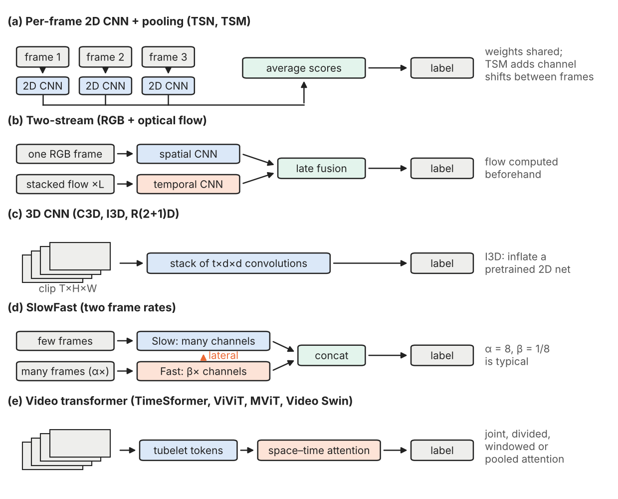
Plain version. Video models combine frame features through pooling, optical flow, temporal convolutions, multiple frame rates or space–time attention.
Per-frame networks and late fusion
The simplest video model applies an image classifier to frames and averages the class scores:
where is the vector of class scores (logits) for one frame and the number of classes. This is order-blind: shuffling the frames gives the same answer, so it cannot tell “opening” from “closing”. It is still a strong baseline on scene-heavy datasets, and it is cheap and can start from any pretrained image backbone (DLCV 02). A recurrent network such as an LSTM [11] over per-frame features adds order; this design is discussed in ML 04.
Two-stream networks: appearance plus optical flow
Plain version. A two-stream model combines appearance from color frames with motion from optical-flow fields.
Simonyan and Zisserman’s two-stream ConvNet [12] has a spatial stream, an image CNN on one RGB frame, and a temporal stream, a CNN whose input is the dense optical flow of consecutive frame pairs. Each flow field has a horizontal component and a vertical component , so the stacked input for frame has channels:
where is a pixel position and , are the horizontal and vertical displacements of that pixel from frame to frame . The two streams are trained separately and fused late, by averaging their softmax scores or with a linear SVM on the stacked scores [12]. The paper showed that a ConvNet on stacked flow performs well despite limited training data, and that the two streams are complementary [12].
The weakness is cost: dense optical flow must be computed (and usually stored) for every frame before training, with a classical solver or a flow network (see DLCV 09A.3 for warping with flow). The flow is also not learned for the recognition task. Temporal Segment Networks [13] and I3D [14] still used a flow stream; SlowFast (below) later learned motion end to end from raw frames, without flow, and its authors found it empirically more effective than the two-stream approach [15].
3D convolutions: C3D and I3D inflation
Plain version. Make every filter a small cube that slides over time as well as space. Then the network can learn motion detectors, such as “a bright edge that moves right”, directly from the pixels.
A 3D convolution with kernel computes, for one input and one output channel,
where is the input at frame , row and column (in practice summed over all input channels and with padding at the borders). C3D [16] trained a network of such layers on a large video dataset and found that a homogeneous architecture with small kernels in all layers was among the best; its features with a linear classifier were strong on several benchmarks.
Training 3D networks from scratch needs much more data than existed in 2015. Carreira and Zisserman solved both problems at once in 2017 [14]. They introduced Kinetics, a dataset of 400 human action classes with at least 400 YouTube clips per class, each about 10 seconds long [17], and the Inflated 3D ConvNet (I3D): take a successful 2D image architecture and inflate every filter and pooling kernel into . To start from weights pretrained on ImageNet [18], they made the inflated network give the same response on a “boring video” (one image repeated in time) as the 2D network on the image: repeat each 2D filter times along time and divide by [14]. With the pretrained filter,
so on a constant-in-time input the temporal taps add up to exactly the 2D response. The check below confirms it numerically.
Code · Python · 14 lines
import numpy as np
from scipy.ndimage import correlate

rng = np.random.default_rng(0)
w2d = rng.standard_normal((3, 3))            # a "pretrained" 2D filter
N = 3                                        # temporal size of the inflated filter
w3d = np.repeat(w2d[None] / N, N, axis=0)    # (N, 3, 3): copy N times, divide by N

img = rng.standard_normal((32, 32))
boring = np.repeat(img[None], 8, axis=0)     # an 8-frame "video" of one still image

r2d = correlate(img, w2d, mode="nearest")
r3d = correlate(boring, w3d, mode="nearest")  # 3D filtering over (t, y, x)
print("max |3D response on any frame - 2D response| =", np.abs(r3d - r2d[None]).max())
Output
max |3D response on any frame - 2D response| = 1.7763568394002505e-15The difference is at the level of floating-point rounding. Training then moves the filters away from “constant in time” as they learn motion. The paper’s final model is two-stream I3D, one I3D on RGB and one on flow with predictions averaged, because the authors still found the flow stream valuable [14]. After pretraining on Kinetics, I3D improved considerably on the small UCF101 and HMDB51 benchmarks [14], which helped make “pretrain on Kinetics, fine-tune on the target” the standard video recipe. The same inflation idea reappears in video generators (DLCV 12A), and I3D features are the feature network behind the Fréchet Video Distance [19] (DLCV 12A).
Optional: Quo Vadis: I3D and the Kinetics dataset (in the Paper guides). How the paper compares five architecture families and what its transfer experiments show.
Factorized (2+1)D convolutions
Plain version. A cube-shaped filter can be split into two cheaper steps: first a flat filter that looks within each frame, then a thin filter that looks across frames at each position. With the right width in between, the split has the same number of parameters but an extra nonlinearity, and it trains more easily.
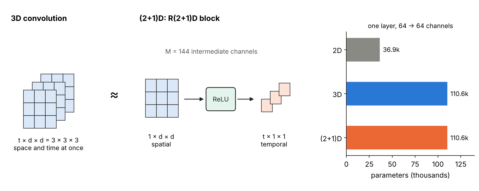
Tran et al. [20] compared several spatiotemporal convolutions inside residual networks: 2D only, 3D everywhere, mixed (3D in early layers only, or late layers only) and a factorized (2+1)D block. The (2+1)D block replaces filters of size with spatial filters of size , a ReLU, and temporal filters of size . Here and are the input and output channel counts of layer , and the temporal and spatial kernel sizes, and the width of the intermediate space, chosen so that the parameter count matches the 3D layer [20]:
The paper names two benefits: the extra ReLU doubles the number of nonlinearities for the same parameter count, and the factorization makes optimization easier, visible as lower training error than an equally sized 3D network [20]. It is the video analogue of the depthwise-separable trick in image CNNs (ML 03): split one big operation into cheaper ones along different axes.
The code computes parameters and multiply–adds for one 64-to-64-channel layer on a 16-frame clip with feature maps, and the token count of a video transformer for comparison.
Code · Python · 24 lines
import math

def conv_cost(c_in, c_out, kt, kh, kw, T, H, W):
    """Parameters and multiply-adds of one convolution (stride 1, 'same' padding, no bias)."""
    params = c_in * c_out * kt * kh * kw
    return params, params * T * H * W

c, t, d = 64, 3, 3                           # channels in = out, temporal and spatial kernel size
T, H, W = 16, 56, 56                         # a 16-frame clip, 56x56 feature maps
M = math.floor(t * d * d * c * c / (d * d * c + t * c))   # R(2+1)D's matched middle width

layers = {
    "2D  (1x3x3), per frame": [conv_cost(c, c, 1, d, d, T, H, W)],
    "3D  (3x3x3)":            [conv_cost(c, c, t, d, d, T, H, W)],
    f"(2+1)D, M={M}":         [conv_cost(c, M, 1, d, d, T, H, W), conv_cost(M, c, t, 1, 1, T, H, W)],
}
for name, parts in layers.items():
    p = sum(x[0] for x in parts); f = sum(x[1] for x in parts)
    print(f"{name:24s} params {p:>8,d}   GMACs {f / 1e9:5.2f}")

# a video transformer's token count with 2x16x16 tubelets on a 16x224x224 clip
n_tok = (16 // 2) * (224 // 16) ** 2
print(f"tokens {n_tok}, joint attention pairs {n_tok**2:,}, "
      f"divided (time, then space) pairs {n_tok * 8 + n_tok * 196:,}")
Output
2D  (1x3x3), per frame   params   36,864   GMACs  1.85
3D  (3x3x3)              params  110,592   GMACs  5.55
(2+1)D, M=144            params  110,592   GMACs  5.55
tokens 1568, joint attention pairs 2,458,624, divided (time, then space) pairs 319,872
With equal input and output widths, makes the (2+1)D block match the 3D layer exactly in parameters and work; the gain is in expressiveness and optimization, not in cost. A cheaper split is possible by choosing a smaller . Figure 4 draws the factorization.
Optional: Choosing the middle width of a (2+1)D block (in the Supplementary notes). Where the formula comes from, and what happens when input and output widths differ or when you want a cheaper block.
Cheap temporal modeling: TSN sampling and the temporal shift module
Plain version. Two tricks let a plain 2D network handle long videos cheaply. TSN looks at a few frames spread over the whole video instead of many frames from one moment. TSM lets neighboring frames swap a few feature channels inside the network, which mixes information across time at almost no cost.
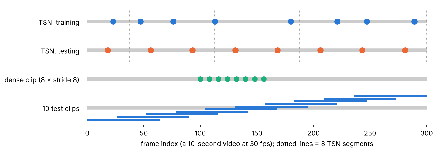
Temporal Segment Networks (TSN) [13] divide a video into equal segments, take one short snippet from each (a random position during training), score every snippet with the same network, and combine the scores with a segmental consensus such as averaging before the softmax. The loss is computed on the consensus, so the whole video supervises the network, not just one short window [13]. The paper’s default was segments [13]. This sparse sampling covers long-range structure with a fixed, small number of frames (Figure 5).
Code · Python · 22 lines
import numpy as np

def tsn_indices(n_frames, K, train, rng=None):
    """TSN-style sparse sampling: split the video into K equal segments, take one frame
    per segment (random position when training, the segment centre when testing)."""
    edges = np.linspace(0, n_frames, K + 1)
    if train:
        return np.floor(edges[:-1] + rng.random(K) * np.diff(edges)).astype(int)
    return np.floor((edges[:-1] + edges[1:]) / 2).astype(int)

def dense_clip(n_frames, length, stride, start):
    """A dense clip: `length` frames, `stride` apart, starting at `start`."""
    return start + stride * np.arange(length)

rng = np.random.default_rng(0)
n = 300                                          # a 10-second video at 30 fps
print("TSN train:", tsn_indices(n, 8, True, rng))
print("TSN test :", tsn_indices(n, 8, False))
print("dense 8x8:", dense_clip(n, 8, 8, start=100))   # 8 frames, every 8th frame
# multi-view testing: 10 clip start positions spread uniformly over the video
starts = np.linspace(0, n - 8 * 8, 10).astype(int)
print("10 clip starts:", starts)
Output
TSN train: [ 23  47  76 113 180 221 247 289]
TSN test : [ 18  56  93 131 168 206 243 281]
dense 8x8: [100 108 116 124 132 140 148 156]
10 clip starts: [  0  26  52  78 104 131 157 183 209 236]
The eight sparse frames span the whole video; the dense clip covers about 2 seconds in detail. (Taking segment centres at test time is a common choice in later implementations; the original TSN paper tested on 25 frames with 10 crops each [13].) Dense clips are what 3D networks and SlowFast consume; the last line, ten clips spread over the video, is the multi-view testing protocol discussed under evaluation below.
The Temporal Shift Module (TSM) [21] adds real temporal interaction to a 2D network with zero extra parameters and zero extra multiply–adds. Inside each residual block, a fraction of the channels of the feature tensor is shifted by one frame forward in time, another fraction one frame backward, and the rest stay in place; the following 2D convolution then mixes channels that come from three different frames. Shifting most channels hurt both latency (data movement) and accuracy (less spatial information per frame), so the paper shifts 1/4 of the channels (1/8 in each direction) and places the shift on the residual branch [21]. For live video, a uni-directional version shifts only from past to current frames [21].
Optional: The temporal shift as a sparse temporal convolution (in the Supplementary notes). A short derivation and a tested snippet showing that shift plus a 1×1 convolution equals a temporal convolution with most weights fixed to zero.
SlowFast: two frame rates
Plain version. What things are changes slowly; how they move can change fast. So use two pathways: a heavy one that looks at few frames to understand the scene, and a light one that looks at many frames to catch the motion.
SlowFast networks [15] have a Slow pathway that samples frames with a large temporal stride , and a Fast pathway that samples frames with stride , so it is times denser in time. The Fast pathway has only a fraction of the Slow pathway’s channels. Typical values are and [15]. Because the cost of a layer grows roughly with the square of its channel count, the Fast pathway takes only about 20% of the total computation in the paper’s instantiations [15]. Lateral connections feed Fast features into the Slow pathway at every stage; to match shapes they convert the Fast frames to , for example with a time-strided 3D convolution, the paper’s default [15].
Two design details carry a general lesson. The Slow pathway uses temporal kernels larger than 1 only in its last two stages, because the authors found that temporal convolutions in early layers hurt when the frame stride is large: fast-moving content has little correlation across a large time step unless the spatial receptive field is also large [15]. And SlowFast uses no optical flow: it learns motion end to end from raw frames [15]. It reported strong results on Kinetics, Charades and AVA classification and detection [15].
Optional: SlowFast networks (in the Paper guides). How to read its ablations on lateral connections and on the channel ratio β.
Two related ideas complete the CNN family. Non-local blocks [22] compute each position’s response as a weighted sum over all space–time positions, an attention layer inserted into a 3D CNN to capture long-range dependencies. X3D [23] starts from a tiny 2D image network and expands it one axis at a time (in space, time, width and depth) to find accurate networks at low cost; one surprising finding was that networks with high spatiotemporal resolution can be extremely thin [23].
Video transformers: TimeSformer, ViViT, MViT and Video Swin
Plain version. Cut the clip into small space–time patches, turn each into a token, and let a transformer decide which patches should look at which. The hard part is that a clip has thousands of tokens, so the designs differ mainly in which tokens each token may attend to.
A Vision Transformer [24] (ML 05) turns an image into patches. A video transformer does the same in space–time. With tubelet embedding [25], non-overlapping tubes of pixels are linearly projected (equivalently, a 3D convolution with stride equal to its kernel), so a clip becomes
tokens, where is the tubelet length in frames and the patch side in pixels. VideoMAE’s ViT-Base, for example, takes a clip with cubes, giving tokens [10]. Joint space–time attention compares all pairs, which the code above counted as about 2.46 million per layer. Four designs tame this:
- TimeSformer [26] compared several self-attention schemes and found divided attention best among those it tried: within each block, a token first attends to the tokens at the same spatial position in other frames (temporal attention) and then to the tokens of its own frame (spatial attention) [26]. In the configuration above that is about 0.32 million pairs instead of 2.46 million. It can also process clips over one minute long [26]. The cost ratio of joint versus divided attention is derived in DLCV 12A, which also explains why video generators often prefer full attention.
- ViViT [25] proposed four models: joint spatio-temporal attention; a factorised encoder (a spatial transformer per frame, then a temporal transformer over the frame embeddings, a form of late fusion); factorised self-attention inside each block; and factorised dot-product attention, where half of the heads attend over space and half over time. It also showed how to regularize these models and initialize them from pretrained image models so they can be trained on comparatively small datasets [25].
- MViT [27] brings back the multiscale hierarchy of CNNs: stages start at high spatiotemporal resolution with few channels and progressively expand channels while reducing resolution, using pooling attention, which pools the query, key and value sequences inside attention [27].
- Video Swin Transformer [28] argues for locality: attention is computed only inside local 3D windows, which are shifted between consecutive layers so information can cross window borders. It extends the image Swin Transformer [29] (DLCV 02) and starts from pretrained image weights, giving a better speed–accuracy trade-off than global attention [28].
Attention is not the only way to model long clips. VideoMamba [30] adapts the Mamba state-space model [31], whose cost grows linearly with the number of tokens, to video; the underlying selective scan is explained in ML 04.
Learning video representations without labels
Plain version. Labeling video is slow and expensive, but unlabeled video is plentiful. So hide most of a clip and train the network to fill it in; to do that well, it must learn how things look and how they move.
VideoMAE [10] applies masked autoencoding (MAE [32], see ML 06) to video. It masks space–time cubes, encodes only the visible ones with a ViT, and reconstructs the pixels of the masked ones with a light decoder. Two things are specific to video. First, consecutive frames are highly redundant, so the masking ratio can be extremely high: 90% to 95% still works well [10]. Second, if masks are drawn independently per frame, a masked patch can often be copied from the same position in a neighboring frame, an information leakage that makes the task too easy. VideoMAE therefore uses tube masking: the same spatial mask in every frame [10]. The snippet measures the leakage.
Code · Python · 16 lines
import numpy as np

rng = np.random.default_rng(0)
T, P, ratio = 8, 196, 0.9               # 8 token frames of 14x14 patches, 90% masked

def leak(mask):
    """Fraction of masked tokens whose same-position token in a neighbouring frame is visible."""
    vis = ~mask
    nb = np.zeros_like(mask)
    nb[1:] |= vis[:-1]; nb[:-1] |= vis[1:]
    return (mask & nb).sum() / mask.sum()

random_mask = rng.random((T, P)) < ratio                  # independent per token
tube_mask = np.repeat((rng.random(P) < ratio)[None], T, 0) # same spatial mask in every frame
print(f"random masking: {random_mask.mean():.2f} masked, leak {leak(random_mask):.2f}")
print(f"tube masking  : {tube_mask.mean():.2f} masked, leak {leak(tube_mask):.2f}")
Output
random masking: 0.90 masked, leak 0.16
tube masking  : 0.89 masked, leak 0.00
With independent masks, about one masked token in six has a visible twin in an adjacent frame (for interior frames the expected value is ; the first and last frames have only one neighbor). Tube masking removes that shortcut entirely, which is the point: a pretext task is only useful if its shortcuts are closed. VideoMAE also reported strong results on small datasets of a few thousand videos without extra data, found that data quality matters more than data quantity for this kind of pretraining, and noted that the domain shift between pretraining and target data is an important issue [10]. VideoMAE V2 [33] scaled the approach to a billion-parameter ViT with dual masking, which also masks the decoder’s input to save computation.
A second line predicts features instead of pixels. V-JEPA [34] trains video models only with a feature-prediction objective, without pretrained image encoders, text, negative examples or reconstruction, on about 2 million videos, and evaluates them with a frozen backbone on both motion- and appearance-based tasks [34]. Its successor V-JEPA 2 [35] and the JEPA idea are covered in ML 06 and DLCV 13.
Video and language, briefly
Plain version. Instead of a fixed list of action names, describe videos with free text. A model that places videos and sentences in the same space can search videos by description; a model that feeds video tokens into a language model can answer questions about them.
Retrieval. CLIP-style image–text models [36] (ML 10) transfer to video: CLIP4Clip [37] transfers CLIP to text–video retrieval end to end and studies whether image features are enough, how post-pretraining on video–text data helps and how to model the dependency between frames, on benchmarks such as MSR-VTT, a collection of 10K web video clips with 200K clip–sentence pairs [38]. Video foundation models such as InternVideo2 [39] combine masked video modeling, video–text contrastive learning and next-token prediction in one progressive training scheme, with a video encoder of up to 6 billion parameters [39].
Question answering. Multimodal large language models (ML 10) accept sampled frames as visual tokens. Long videos stress them: Video-MME [40] evaluates them on 900 manually annotated videos from 11 seconds to 1 hour long (2,700 question–answer pairs), with subtitles and audio as optional inputs, and found that handling longer sequences remained a weakness [40]. A practical caution, by analogy with scene bias: check whether a question can be answered from a single frame, or from the question text alone, before crediting a model with temporal understanding; a single-frame baseline is a cheap sanity check.
Localizing actions in time and space
Plain version. Real videos are not trimmed. A cooking video contains “cut”, “stir” and “pour” with long boring stretches in between. Temporal localization finds where each action starts and ends; spatio-temporal detection also says which person is doing it.
Temporal action localization
The task mirrors object detection along the time axis (DLCV 03), and so do its methods. A clip-level backbone (often frozen, such as I3D or SlowFast features) produces a feature sequence along time; a localization head turns it into scored segments.
- Proposal-based (two-stage). First generate class-agnostic candidate segments, then classify them. BMN [41] represents a proposal as a pair of start and end boundaries and scores all densely distributed pairs at once in a boundary-matching confidence map; combined with an action classifier it gives detections [41].
- Anchor-free, single-stage. ActionFormer [42] classifies every moment in time and regresses the distances to the action’s start and end, with no proposals and no predefined anchor windows. It uses a multiscale transformer with local self-attention and a light decoder [42], the temporal counterpart of the anchor-free detectors of DLCV 03. Duplicate segments are removed with non-maximum suppression in time, as for boxes (ActionFormer uses a soft variant [42]).
Temporal IoU and mAP. For a predicted segment and a ground-truth segment ,
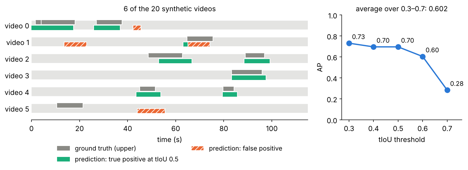
where the numerator is the length of the overlap and the denominator the length of the union. For one class and threshold , predictions are sorted by score; a prediction is a true positive if its tIoU with a not-yet-matched ground truth of that class is at least . Average precision (AP) is the area under the resulting precision–recall curve, mAP averages AP over classes, and an average mAP averages over several thresholds. Two conventions are common: THUMOS14 averages over tIoU and ActivityNet 1.3 over [42]. The code computes AP for one class on synthetic detections (85% of actions found, with boundary errors, plus random false alarms).
Code · Python · 46 lines
import numpy as np

def tiou(seg, segs):
    """Temporal IoU of one segment [s, e] with an array of segments (n, 2)."""
    inter = np.clip(np.minimum(seg[1], segs[:, 1]) - np.maximum(seg[0], segs[:, 0]), 0, None)
    union = (seg[1] - seg[0]) + (segs[:, 1] - segs[:, 0]) - inter
    return inter / union

def average_precision(preds, gts, thr):
    """preds: list of (video, start, end, score); gts: dict video -> (m, 2) array.
    Greedy matching in score order; each ground truth can be matched once."""
    n_gt = sum(len(g) for g in gts.values())
    used = {v: np.zeros(len(g), bool) for v, g in gts.items()}
    tp = []
    for v, s, e, _ in sorted(preds, key=lambda p: -p[3]):
        ious = tiou(np.array([s, e]), gts[v])
        ious[used[v]] = -1                       # already matched ground truths are off limits
        j = int(np.argmax(ious))
        hit = ious[j] >= thr
        if hit:
            used[v][j] = True
        tp.append(hit)
    tp = np.array(tp, float)
    recall = np.cumsum(tp) / n_gt
    precision = np.cumsum(tp) / np.arange(1, len(tp) + 1)
    precision = np.maximum.accumulate(precision[::-1])[::-1]   # monotone envelope
    return np.sum(np.diff(np.r_[0, recall]) * precision)

rng = np.random.default_rng(0)
gts, preds = {}, []
for v in range(20):                              # 20 untrimmed videos, 1-3 actions each
    starts = np.sort(rng.uniform(0, 100, rng.integers(1, 4)))
    g = np.c_[starts, starts + rng.uniform(4, 15, len(starts))]
    gts[v] = g
    for s, e in g:
        if rng.random() < 0.85:                  # the detector finds 85% of actions...
            j = rng.normal(0, 0.2 * (e - s), 2)  # ...with boundary errors
            preds.append((v, s + j[0], e + j[1], rng.uniform(0.5, 1.0)))
    for _ in range(rng.integers(0, 3)):          # plus some false alarms
        s = rng.uniform(0, 100)
        preds.append((v, s, s + rng.uniform(3, 12), rng.uniform(0.0, 0.7)))

thrs = [0.3, 0.4, 0.5, 0.6, 0.7]
aps = [average_precision(preds, gts, t) for t in thrs]
print("AP at tIoU:", "  ".join(f"{t}: {a:.3f}" for t, a in zip(thrs, aps)))
print(f"average over [0.3:0.1:0.7]: {np.mean(aps):.3f}")
Output
AP at tIoU: 0.3: 0.731  0.4: 0.696  0.5: 0.696  0.6: 0.604  0.7: 0.284
average over [0.3:0.1:0.7]: 0.602
(Toy numbers.) Up to tIoU 0.5 the AP is limited mainly by the 15% missed actions and the false alarms; at 0.7 it collapses because boundary errors of about 20% of the action length are no longer good enough. Boundaries of actions are genuinely ambiguous (when does “pour” start?), which is why strict thresholds are hard even for people, and why benchmarks report several.
Optional: Average precision for temporal localization, step by step (in the Supplementary notes). A hand-worked example of the matching rule, duplicates and the precision envelope.
Spatio-temporal action detection
Here the model must say which person does which action. In AVA [43], every person in keyframes sampled at 1 Hz from 15-minute movie clips gets a box and one or more labels from 80 atomic actions (14 pose classes, 49 person–object and 17 person–person interactions) [43]. A common pipeline is detection plus video classification, as in SlowFast’s AVA detector [15]: an off-the-shelf person detector (DLCV 03) proposes boxes on the keyframe, a video backbone computes a spatiotemporal feature map for a clip around it, the features inside each box are pooled, and a per-class sigmoid classifier gives multi-label predictions, because one person can “stand”, “talk to” and “hold” at once. The metric is frame-mAP at IoU 0.5: AP per action class over all keyframe detections, a detection counting only if its box overlaps a ground-truth box of that class with IoU at least 0.5, averaged over classes [43]. Linking detections into tubes over time borrows the association methods of tracking (DLCV 07).
Skeleton-based action recognition
Instead of pixels, a model can read the pose: the 2D or 3D coordinates of body joints over time, estimated as in DLCV 05 or captured with depth sensors, as in the NTU RGB+D dataset of 60 action classes [44]. ST-GCN [45] builds a graph whose nodes are the joints in every frame, with spatial edges along the bones and temporal edges connecting the same joint in consecutive frames, and applies graph convolutions over it [45]. Skeletons are compact, ignore clothing and background, and are therefore less prone to scene bias: on the Mimetics dataset of mimed actions without the usual objects and scenes, a pose-based model held up much better than 3D CNNs [46]. The price is that skeletons miss objects (“drinking” versus “eating”) and depend on the pose estimator’s errors.
Optional: Graph convolution on a skeleton sequence (ST-GCN) (in the Supplementary notes). The normalized adjacency, the partition of neighbors and how the convolution is implemented.
Training and evaluating video classifiers
Plain version. How you pick frames, how many views you average at test time and which dataset you report on change the numbers as much as many architecture changes. Read the protocol before comparing two papers.
Sampling and training
Three choices define the input: the number of frames , the stride between them (frame rate), and dense versus sparse (TSN-style) sampling. Motion-centric datasets reward dense, fine-grained sampling; scene-centric datasets tolerate sparse sampling. VideoMAE, for example, uses TSN-style uniform sampling on Something-Something V2 and dense sampling on Kinetics-400 [10]. Spatial augmentation is the same as for images (random resized crops, flips), with one video-specific trap: horizontal flipping changes the label of direction-dependent classes such as “pushing something from left to right”. Training otherwise follows DLCV 02. Initialization usually comes from an image model (inflation, or a pretrained ViT) or from a self-supervised video model.
Multi-view testing
At test time, one clip rarely covers the whole video, so predictions are averaged over temporal clips and spatial crops:
where is the -th clip cropped at the -th spatial position. SlowFast, for example, samples 10 clips uniformly along the video and takes 3 crops of from each, 30 views in total, and reports cost as GFLOPs per view × number of views, noting that some earlier works used more than 100 views [15]. VideoMAE evaluated with 2 clips × 3 crops on Something-Something V2 and 5 × 3 on Kinetics-400 [10]. The total inference cost is the per-view cost times the number of views, so a model that looks cheap per view may be expensive in practice. Report both, and compare models only under the same protocol.
Datasets and benchmarks
| Dataset | Task | Content (as described by its authors) |
|---|---|---|
| UCF101 [47] | clip classification | 101 action classes, over 13k clips, 27 hours of user-uploaded video |
| HMDB51 [48] | clip classification | 51 action classes from movies and web videos; small and deliberately hard |
| Kinetics-400 [17] | clip classification | 400 human action classes, at least 400 clips each, about 10 s per clip, from YouTube |
| Something-Something V2 [9], [10] | clip classification | 174 motion-centric classes defined as caption templates; about 169k training and 20k validation videos |
| Diving48 [7] | clip classification | over 18,000 clips of 48 fine-grained dive classes, built to reduce static bias |
| Charades [49] | multi-label classification, localization | 9,848 videos of everyday indoor activities recorded by 267 people, 157 action classes |
| THUMOS14 [50] | temporal localization | untrimmed videos, including background videos without the target actions |
| ActivityNet [51] | untrimmed classification, localization | a large-scale benchmark of human activities in untrimmed web videos |
| AVA [43] | spatio-temporal detection | 80 atomic actions in 430 15-minute movie clips, 1.58M action labels |
| EPIC-KITCHENS-100 [52], [53] | egocentric recognition, detection, anticipation | 100 hours of unscripted head-mounted video in 45 environments, 90K actions |
| NTU RGB+D [44] | skeleton / RGB-D recognition | over 56 thousand samples, 60 action classes, 40 subjects |
| MSR-VTT [38] | retrieval, captioning | 10K web clips, 200K clip–sentence pairs |
| Video-MME [40] | video QA for multimodal LLMs | 900 videos from 11 s to 1 h, 2,700 question–answer pairs |
UCF101 and HMDB51 report average accuracy over three official train/test splits [12], [13]; Kinetics and Something-Something report top-1 and top-5 on their validation sets; Charades and AVA report mAP. Two warnings. First, Kinetics and Something-Something reward different things: the VideoMAE authors describe Kinetics videos as mostly stationary and scene-related, while Something-Something V2 is motion-centric [10]. A model’s ranking can change between them. Second, the authors of EPIC-KITCHENS-100 built in a “test of time”: testing models trained on footage collected in 2018 on new footage collected two years later, and an unsupervised domain adaptation challenge [53]. Benchmarks like these measure robustness that a single held-out split cannot.
Failure modes
Plain version. Video models fail in a few predictable ways. Most of them come from the model using a cue that happened to work on the training data.
- Scene and object bias. The model predicts “playing tennis” from a tennis court. Evidence: representation bias toward static cues in common datasets [7]; models that fail on mimed actions without the usual objects and scenes [46]. Remedies include debiasing losses, such as an adversarial scene classifier and a loss that penalizes confident predictions on videos with the person masked out [54], motion-centric training data [9] and pose input [46].
- Temporal shortcuts. The model ignores frame order. Test: shuffle or reverse the frames. If accuracy barely moves, the model (or the benchmark) does not use time; Sevilla-Lara et al. built their temporal subset of classes exactly this way [8].
- Short temporal context. Most clip models see only a few seconds at a time. Actions defined over minutes (“assembling furniture”) or questions about a whole film need long-range memory, which remains a weakness even for large multimodal models [40].
- Domain shift. Third-person YouTube video, egocentric kitchens, surveillance at night and medical endoscopy look very different. Models trained on one transfer imperfectly to another; EPIC-KITCHENS-100 measures this with unseen kitchens and footage recorded later [52], [53]. Distribution-shift tests from DLCV 02 apply.
- Ambiguous labels and boundaries. Actions overlap, have fuzzy starts and ends and depend on intent. Multi-label datasets (Charades, AVA) and several tIoU thresholds acknowledge this; single-label accuracy hides it.
- Unfair comparisons. Different numbers of views, frame counts, resolutions and pretraining data make reported numbers incomparable [1]. Always check the protocol line of a results table.
Two cheap diagnostics catch most of these: a single-frame baseline (how much of the score needs no time at all?) and a shuffled-frames test (does order matter to the model?). Run both before trusting a video model.
Modern view
What the surveys say
Five surveys cover the field from different angles. Zhu et al. [1] review over 200 papers on deep action recognition, introduce 17 datasets, present the models in chronological order (early attempts, two-stream networks, 3D convolutions, compute-efficient models), benchmark popular methods under one protocol with released code, and name the field’s main challenges: long-range temporal modeling, compute cost and results made incomparable by different datasets and protocols. Kong and Fu [2] cover both recognition (labeling a complete action) and prediction (anticipating an action from its first part), including datasets and evaluation protocols. Selva et al. [3] organize video transformers by how they tokenize the input, how they reduce redundancy and reintroduce inductive biases, how they capture long-term dynamics and how they are trained, and find that they outperform 3D CNNs on action classification even at lower computational cost. Madan et al. [4] analyze over 200 video foundation models in three groups (image-based models adapted to video, video-based models, and universal models across modalities) and report that image-based models outperform video-based ones on most video understanding tasks, while universal multimodal models do best. Tang et al. [5] categorize video understanding with large language models by how the video reaches the language model (video analyzer, video embedder or both) and by the role of the language model (summarizer, manager, text decoder, regressor or hidden layer).
Optional: Guide to the Modern view surveys (in the Paper guides). How each survey is organized and what to read first.
The state of the art, 2023–2026
- Self-supervised pretraining is a common starting point. Masked video modeling (VideoMAE [10], VideoMAE V2 [33]) and feature prediction (V-JEPA [34]) produce encoders that are fine-tuned or probed for downstream tasks; the VideoMAE V2 authors call scale the primary factor for such foundation models [33].
- Video foundation models unify tasks. Models such as InternVideo2 [39] train one encoder with masked modeling, video–text contrast and next-token prediction, and are evaluated across recognition, retrieval and dialogue. The finding of Madan et al. that adapted image models remain very competitive [4] is a reminder that much of video understanding is still appearance.
- Multimodal LLMs take over open-ended understanding. Video question answering, captioning and temporal grounding are increasingly handled by language models with visual tokens, evaluated on benchmarks such as Video-MME [40]. The bottleneck is the number of visual tokens for long videos.
- Efficient long-range models. Linear-cost sequence models such as VideoMamba [30] and streaming designs (in the spirit of online TSM [21]) target long and live video.
- Localization builds on pretrained encoders. Temporal localizers run on features from pretrained video models; ActionFormer, for example, uses two-stream I3D features pretrained on Kinetics for THUMOS14 [42], so better encoders and better localization heads improve results together.
Open problems
- Genuine temporal reasoning. Benchmarks where one frame or the language prior is not enough, and models that use order, causality and duration.
- Long video. Memory and token budgets for hours of video, and evaluation of long-range understanding.
- Fine-grained and egocentric actions. Hands, small objects, and intent; transfer across viewpoints and environments.
- Efficient and online recognition. Low latency on devices, with honest cost reporting (FLOPs × views, real latency).
- Evaluation. Comparable protocols, contamination of benchmarks by web-scale pretraining data, and metrics that reward temporal understanding rather than appearance.
Key takeaways
- Choose metrics from the requested output: clip labels, action intervals, person boxes or retrieval results.
- A strong score can reflect scene cues rather than motion understanding.
- Flow, temporal convolutions and attention incorporate time differently; inspect what information each can access.
- Sampling and multi-rate pathways trade temporal coverage against computation.
- Masking must prevent easy temporal leakage if pretraining is meant to learn useful structure.
- Compare matched testing views and pretraining, then test a single-frame baseline and shuffled-frame inputs.
Exercises
- How much does the combined model cheat? In the scene-bias code, standardize the features (
sklearn.preprocessing.StandardScalerin a pipeline) and varyCover 0.01, 0.1 and 1. How do the “no cue” and “shift” accuracies of the frame+motion model change? Why does standardization help it use the motion feature?
Hint
The motion features have a small numeric range compared with the 400 pixel features, so with an L2 penalty the model finds it cheaper to spread weight over many pixels. In our runs, standardizing gave the frame+motion model “no cue”/“shift” accuracies of 0.752/0.547 at C = 0.01, 0.824/0.685 at C = 0.1 and 0.842/0.708 at C = 1, still well below the motion-only model. Scaling reduces the shortcut but does not remove it while the scene remains predictive in training.
- Inflation by hand. A 2D filter (a horizontal derivative) is inflated to frames. Write , and compute its response at one position for (a) a boring video where every frame has the row and (b) a video whose three frames have rows , and . What does the difference tell you about what training must change?
Hint
has three temporal slices, each . (a) Each slice gives , total , the same as the 2D response. (b) The slices give , and , total . The inflated filter averages the frames, so it responds to motion only through blurring; to become a motion detector, training must make the temporal slices different (for example, opposite signs on the first and last).
- (2+1)D with unequal widths. For a layer with input and output channels, , , compute , the 3D parameter count and the (2+1)D parameter count. Then choose and compute the savings.
Hint
. 3D: . (2+1)D with : (slightly less, because of the floor). With : , about 28% of the 3D layer.
- Views and cost. Model A costs 36 GFLOPs per view and is tested with 10 × 3 views; model B costs 180 GFLOPs per view and is tested with 1 × 3 views. Which is more expensive per video? Design a fair comparison.
Hint
A: GFLOPs; B: GFLOPs, so A costs twice as much per video despite being five times cheaper per view. A fair comparison plots accuracy against total inference cost for several view counts of each model, on the same frames and resolution.
- A shuffled-frames test. Extend the scene-bias code: shuffle the frame order of each test clip, with a new permutation per clip (
rng = np.random.default_rng(5), thennp.stack([x[rng.permutation(8)] for x in X])), and re-evaluate the three models trained on ordered clips. Predict the result before you run it.
Hint
The one-frame model still reads only the scene, so it barely changes (0.868 / 0.499 / 0.127 on the three test sets in our run). The motion model’s per-pair estimates now have random signs, and it drops to chance (0.522 / 0.500 / 0.466). The frame+motion model does not move (0.864 / 0.497 / 0.133), which exposes that it never relied on order. A model whose accuracy survives shuffling is not using time.
- tIoU by hand. A ground-truth action runs from 10 s to 20 s. Predictions: P1 [12, 22] with score 0.9, P2 [9, 19] with score 0.8, P3 [30, 35] with score 0.7. Compute each tIoU, mark TP/FP at and , and compute AP at both thresholds.
Hint
P1: overlap 8, union 12, tIoU 0.667. P2: overlap 9, union 11, tIoU 0.818. P3: 0. At 0.5: P1 is TP (first in score order), P2 is a duplicate (FP), P3 FP; precision at recall 1 is 1, so AP = 1. At 0.75: P1 is FP, P2 is TP (precision 1/2 at recall 1), P3 FP; AP = 0.5. A worse box with a higher score can cost half the AP at a strict threshold.
References
- Y. Zhu, X. Li, C. Liu, M. Zolfaghari, Y. Xiong, C. Wu, Z. Zhang, J. Tighe et al., “A comprehensive study of deep video action recognition,” technical report, arXiv:2012.06567, 2020. arXiv
- Y. Kong and Y. Fu, “Human action recognition and prediction: A survey,” International Journal of Computer Vision, vol. 130, no. 5, pp. 1366–1401, 2022. doi
- J. Selva, A. S. Johansen, S. Escalera, K. Nasrollahi, T. B. Moeslund and A. Clapés, “Video transformers: A survey,” IEEE Transactions on Pattern Analysis and Machine Intelligence, vol. 45, no. 11, pp. 12922–12943, 2023. doi
- N. Madan, A. Moegelmose, R. Modi, Y. S. Rawat and T. B. Moeslund, “Foundation models for video understanding: A survey,” arXiv:2405.03770, 2024. arXiv
- Y. Tang, J. Bi, S. Xu, L. Song, S. Liang, T. Wang, D. Zhang, J. An et al., “Video understanding with large language models: A survey,” arXiv:2312.17432, 2023 (accepted to IEEE Transactions on Circuits and Systems for Video Technology according to the arXiv record). arXiv
- A. Karpathy, G. Toderici, S. Shetty, T. Leung, R. Sukthankar and L. Fei-Fei, “Large-scale video classification with convolutional neural networks,” in Proc. IEEE CVPR, pp. 1725–1732, 2014. CVF
- Y. Li, Y. Li and N. Vasconcelos, “RESOUND: Towards action recognition without representation bias,” in Proc. ECCV, 2018. CVF
- L. Sevilla-Lara, S. Zha, Z. Yan, V. Goswami, M. Feiszli and L. Torresani, “Only time can tell: Discovering temporal data for temporal modeling,” in Proc. IEEE WACV, 2021. doi
- R. Goyal, S. Ebrahimi Kahou, V. Michalski, J. Materzyńska, S. Westphal, H. Kim, V. Haenel, I. Fruend et al., “The ‘something something’ video database for learning and evaluating visual common sense,” in Proc. IEEE ICCV, 2017. CVF
- Z. Tong, Y. Song, J. Wang and L. Wang, “VideoMAE: Masked autoencoders are data-efficient learners for self-supervised video pre-training,” in Advances in Neural Information Processing Systems (NeurIPS), 2022. NeurIPS · arXiv
- S. Hochreiter and J. Schmidhuber, “Long short-term memory,” Neural Computation, vol. 9, no. 8, pp. 1735–1780, 1997. doi
- K. Simonyan and A. Zisserman, “Two-stream convolutional networks for action recognition in videos,” in Advances in Neural Information Processing Systems (NeurIPS), 2014. NeurIPS · arXiv
- L. Wang, Y. Xiong, Z. Wang, Y. Qiao, D. Lin, X. Tang and L. Van Gool, “Temporal segment networks: Towards good practices for deep action recognition,” in Proc. ECCV, pp. 20–36, 2016. doi · arXiv
- J. Carreira and A. Zisserman, “Quo vadis, action recognition? A new model and the Kinetics dataset,” in Proc. IEEE CVPR, 2017. CVF · arXiv
- C. Feichtenhofer, H. Fan, J. Malik and K. He, “SlowFast networks for video recognition,” in Proc. IEEE/CVF ICCV, 2019. CVF · arXiv
- D. Tran, L. Bourdev, R. Fergus, L. Torresani and M. Paluri, “Learning spatiotemporal features with 3D convolutional networks,” in Proc. IEEE ICCV, pp. 4489–4497, 2015. CVF
- W. Kay, J. Carreira, K. Simonyan, B. Zhang, C. Hillier, S. Vijayanarasimhan, F. Viola, T. Green et al., “The Kinetics human action video dataset,” arXiv:1705.06950, 2017. arXiv
- J. Deng, W. Dong, R. Socher, L.-J. Li, K. Li and L. Fei-Fei, “ImageNet: A large-scale hierarchical image database,” in Proc. IEEE CVPR, 2009. doi
- T. Unterthiner, S. van Steenkiste, K. Kurach, R. Marinier, M. Michalski and S. Gelly, “Towards accurate generative models of video: A new metric & challenges,” arXiv:1812.01717, 2018. arXiv
- D. Tran, H. Wang, L. Torresani, J. Ray, Y. LeCun and M. Paluri, “A closer look at spatiotemporal convolutions for action recognition,” in Proc. IEEE/CVF CVPR, 2018. CVF · arXiv
- J. Lin, C. Gan and S. Han, “TSM: Temporal shift module for efficient video understanding,” in Proc. IEEE/CVF ICCV, 2019. CVF · arXiv
- X. Wang, R. Girshick, A. Gupta and K. He, “Non-local neural networks,” in Proc. IEEE/CVF CVPR, 2018. CVF
- C. Feichtenhofer, “X3D: Expanding architectures for efficient video recognition,” in Proc. IEEE/CVF CVPR, 2020. CVF
- A. Dosovitskiy, L. Beyer, A. Kolesnikov, D. Weissenborn, X. Zhai, T. Unterthiner, M. Dehghani, M. Minderer et al., “An image is worth 16x16 words: Transformers for image recognition at scale,” in Proc. ICLR, 2021. arXiv
- A. Arnab, M. Dehghani, G. Heigold, C. Sun, M. Lučić and C. Schmid, “ViViT: A video vision transformer,” in Proc. IEEE/CVF ICCV, 2021. CVF · arXiv
- G. Bertasius, H. Wang and L. Torresani, “Is space-time attention all you need for video understanding?,” in Proc. ICML, PMLR 139, 2021. PMLR · arXiv
- H. Fan, B. Xiong, K. Mangalam, Y. Li, Z. Yan, J. Malik and C. Feichtenhofer, “Multiscale vision transformers,” in Proc. IEEE/CVF ICCV, 2021. CVF · arXiv
- Z. Liu, J. Ning, Y. Cao, Y. Wei, Z. Zhang, S. Lin and H. Hu, “Video Swin Transformer,” in Proc. IEEE/CVF CVPR, 2022. CVF · arXiv
- Z. Liu, Y. Lin, Y. Cao, H. Hu, Y. Wei, Z. Zhang, S. Lin and B. Guo, “Swin Transformer: Hierarchical vision transformer using shifted windows,” in Proc. IEEE/CVF ICCV, 2021. doi
- K. Li, X. Li, Y. Wang, Y. He, Y. Wang, L. Wang and Y. Qiao, “VideoMamba: State space model for efficient video understanding,” in Proc. ECCV, pp. 237–255, 2024. doi · arXiv
- A. Gu and T. Dao, “Mamba: Linear-time sequence modeling with selective state spaces,” in Proc. Conference on Language Modeling (COLM), 2024. arXiv
- K. He, X. Chen, S. Xie, Y. Li, P. Dollár and R. Girshick, “Masked autoencoders are scalable vision learners,” in Proc. IEEE/CVF CVPR, 2022. doi
- L. Wang, B. Huang, Z. Zhao, Z. Tong, Y. He, Y. Wang, Y. Wang and Y. Qiao, “VideoMAE V2: Scaling video masked autoencoders with dual masking,” in Proc. IEEE/CVF CVPR, 2023. CVF · arXiv
- A. Bardes, Q. Garrido, J. Ponce, X. Chen, M. Rabbat, Y. LeCun, M. Assran and N. Ballas, “Revisiting feature prediction for learning visual representations from video,” Transactions on Machine Learning Research (TMLR), 2024. OpenReview · arXiv
- M. Assran, A. Bardes, D. Fan, Q. Garrido, R. Howes et al., “V-JEPA 2: Self-supervised video models enable understanding, prediction and planning,” arXiv:2506.09985, 2025. arXiv
- A. Radford, J. W. Kim, C. Hallacy, A. Ramesh, G. Goh, S. Agarwal et al., “Learning transferable visual models from natural language supervision,” in Proc. ICML, PMLR 139, 2021. PMLR
- H. Luo, L. Ji, M. Zhong, Y. Chen, W. Lei, N. Duan and T. Li, “CLIP4Clip: An empirical study of CLIP for end to end video clip retrieval and captioning,” Neurocomputing, vol. 508, pp. 293–304, 2022. doi · arXiv
- J. Xu, T. Mei, T. Yao and Y. Rui, “MSR-VTT: A large video description dataset for bridging video and language,” in Proc. IEEE CVPR, 2016. CVF
- Y. Wang, K. Li, X. Li, J. Yu, Y. He, G. Chen, B. Pei, R. Zheng et al., “InternVideo2: Scaling foundation models for multimodal video understanding,” in Proc. ECCV, pp. 396–416, 2024. doi · arXiv
- C. Fu, Y. Dai, Y. Luo, L. Li, S. Ren, R. Zhang, Z. Wang, C. Zhou et al., “Video-MME: The first-ever comprehensive evaluation benchmark of multi-modal LLMs in video analysis,” in Proc. IEEE/CVF CVPR, 2025. CVF · arXiv
- T. Lin, X. Liu, X. Li, E. Ding and S. Wen, “BMN: Boundary-matching network for temporal action proposal generation,” in Proc. IEEE/CVF ICCV, 2019. CVF
- C.-L. Zhang, J. Wu and Y. Li, “ActionFormer: Localizing moments of actions with transformers,” in Proc. ECCV, pp. 492–510, 2022. doi · arXiv
- C. Gu, C. Sun, D. A. Ross, C. Vondrick, C. Pantofaru, Y. Li, S. Vijayanarasimhan, G. Toderici et al., “AVA: A video dataset of spatio-temporally localized atomic visual actions,” in Proc. IEEE/CVF CVPR, 2018. CVF · arXiv
- A. Shahroudy, J. Liu, T.-T. Ng and G. Wang, “NTU RGB+D: A large scale dataset for 3D human activity analysis,” in Proc. IEEE CVPR, 2016. doi · arXiv
- S. Yan, Y. Xiong and D. Lin, “Spatial temporal graph convolutional networks for skeleton-based action recognition,” in Proc. AAAI, vol. 32, no. 1, 2018. doi · arXiv
- P. Weinzaepfel and G. Rogez, “Mimetics: Towards understanding human actions out of context,” International Journal of Computer Vision, vol. 129, no. 5, pp. 1675–1690, 2021. doi · arXiv
- K. Soomro, A. R. Zamir and M. Shah, “UCF101: A dataset of 101 human actions classes from videos in the wild,” technical report CRCV-TR-12-01, arXiv:1212.0402, 2012. arXiv
- H. Kuehne, H. Jhuang, E. Garrote, T. Poggio and T. Serre, “HMDB: A large video database for human motion recognition,” in Proc. IEEE ICCV, pp. 2556–2563, 2011. doi
- G. A. Sigurdsson, G. Varol, X. Wang, A. Farhadi, I. Laptev and A. Gupta, “Hollywood in homes: Crowdsourcing data collection for activity understanding,” in Proc. ECCV, pp. 510–526, 2016. doi · arXiv
- H. Idrees, A. R. Zamir, Y.-G. Jiang, A. Gorban, I. Laptev, R. Sukthankar and M. Shah, “The THUMOS challenge on action recognition for videos ‘in the wild’,” Computer Vision and Image Understanding, vol. 155, pp. 1–23, 2017. doi
- F. Caba Heilbron, V. Escorcia, B. Ghanem and J. C. Niebles, “ActivityNet: A large-scale video benchmark for human activity understanding,” in Proc. IEEE CVPR, pp. 961–970, 2015. CVF
- D. Damen, H. Doughty, G. M. Farinella, S. Fidler, A. Furnari, E. Kazakos, D. Moltisanti, J. Munro et al., “Scaling egocentric vision: The EPIC-KITCHENS dataset,” in Proc. ECCV, 2018. CVF
- D. Damen, H. Doughty, G. M. Farinella, A. Furnari, E. Kazakos, J. Ma, D. Moltisanti, J. Munro et al., “Rescaling egocentric vision: Collection, pipeline and challenges for EPIC-KITCHENS-100,” International Journal of Computer Vision, vol. 130, no. 1, 2022. doi · arXiv
- J. Choi, C. Gao, J. C. E. Messou and J.-B. Huang, “Why can’t I dance in the mall? Learning to mitigate scene bias in action recognition,” in Advances in Neural Information Processing Systems (NeurIPS), 2019. NeurIPS · arXiv
- C. Szegedy, W. Liu, Y. Jia, P. Sermanet, S. Reed, D. Anguelov, D. Erhan, V. Vanhoucke and A. Rabinovich, “Going deeper with convolutions,” in Proc. IEEE CVPR, 2015. doi
Check your understanding
This tutorial has 6 exercises. Can you solve them without opening the hints?
Go to the exercises ↑Next DLCV 09 · Deep Image Restoration: Low-Level Vision · 57 min