DLCV 03B · 3D Object Detection: LiDAR, Cameras and Bird's-Eye View
Needs: DLCV 03 · Object Detection: From R-CNN to DETR, DLCV 11 · 3D Reconstruction: From Multi-View Geometry to NeRF and Gaussian Splatting
Navigate: this page and this track: Navigate: this page and this track
On this page
- What you’ll learn1 min
- The big picture1 min
- The 3D detection problem4 min
- Point clouds: what the network actually sees2 min
- A classical baseline: ground removal, clustering and box fitting3 min
- 3D boxes: encoding, IoU and NMS4 min
- LiDAR-based detectors7 min
- Camera-only 3D detection4 min
- Fusing LiDAR, cameras and radar2 min
- Training: assignment and augmentation2 min
- Datasets and metrics5 min
- Efficiency and deployment1 min
- Failure modes2 min
- Modern view3 min
- Key takeaways1 min
- Exercises4 min
- Supplementary notes
- Paper guides
- References
Deep Learning for Computer Vision
Explore this chapter 1 interactive experiment
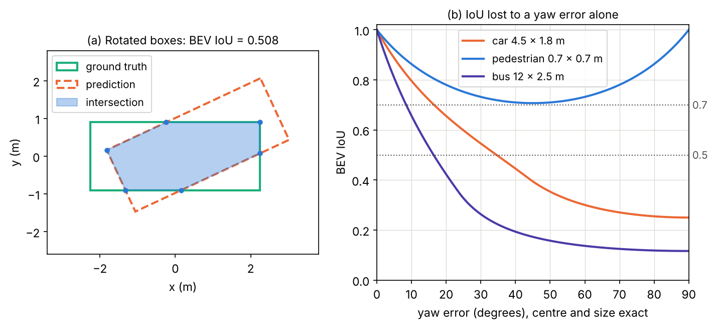
Turn a predicted box a few degrees away from the ground truth in the bird’s-eye view and watch the exact rotated IoU fall while the centre distance stays at zero.
What you’ll learn
- Define 3D boxes, coordinate frames and sensor calibration.
- Compare point, voxel, pillar and hybrid representations.
- Understand camera-only depth inference and multi-sensor fusion.
- Encode orientation and distinguish BEV overlap from full 3D overlap.
- Interpret benchmark metrics and test range, weather, calibration and deployment cost.
The big picture
A 2D detector draws rectangles on an image. A 3D detector places boxes in the real world: where each object is in metres, how big it is, which way it faces and, for moving things, how fast it goes. A self-driving car does not brake for a rectangle of pixels; it brakes because a pedestrian is 14 metres ahead and walking into its lane.
Why it matters. 3D detection is the core of the perception stack in autonomous driving, where it feeds tracking, motion prediction and planning [1]. Robots need it to grasp and avoid objects, and augmented reality needs it to anchor virtual content to real things. The task also forced new ideas that 2D vision never needed: networks for unordered point sets, sparse convolution, the bird’s-eye-view representation, and ways to “lift” flat images into 3D.
This chapter assumes the 2D detection vocabulary of DLCV 03 · Object Detection: box regression targets, IoU, anchors and label assignment, NMS and the focal loss (its core building blocks), centre-based detection (anchor-free detectors), DETR-style set prediction (set prediction with transformers) and average precision (evaluating detectors). We reuse those ideas and only explain what changes in 3D. Two surveys frame the field: Mao et al. [1] and Qian et al. [2]; we return to them in the Modern view.
The 3D detection problem
Plain version. A 3D detector turns sensor observations into boxes, classes and scores. The upright-box setting models yaw while excluding roll and pitch.
Precise version. A 3D detector outputs a set
where is the box centre in metres, are its length, width and height, is the yaw (heading angle about the vertical axis), is one of classes, is a confidence, is an optional ground-plane velocity in metres per second, and varies from scene to scene. This 7-number box is called a 7-DoF (degrees of freedom) box; the Waymo Open Dataset, for example, labels every object this way, with length, width and height measured along the box’s own , and axes [3]. Roll and pitch are assumed to be zero, which is reasonable for road users on a roughly flat road.
Compared with 2D detection, three things change:
- The box lives in metric space. Sizes do not shrink with distance, so a car is about 4.5 m long whether it is 5 m or 80 m away. This makes size priors (anchors, class-average sizes) far more useful than in images.
- Orientation matters. A 2D box is axis-aligned. A 3D box must turn with the object, and a wrong yaw can ruin the overlap even when the centre is perfect.
- The data are sparse and uneven. A LiDAR sees surfaces, not volumes, mostly the sides that face it, and far objects get only a few points.
Sensors and coordinate frames
Plain version. Each sensor measures in its own coordinates. To combine them, we move everything into one shared frame attached to the car, using the known position and orientation of each sensor, its calibration.
Three sensors dominate (Figure 1, left):
- LiDAR sends laser pulses and times their echoes. A spinning unit returns a point cloud: tens of thousands of points per sweep, each with an intensity (reflectance). Depth is measured directly and accurately, but there is no colour, and the points are sparse.
- Cameras give dense colour and texture at low cost but no depth: a pixel tells you the direction of a ray, not how far along the ray the object is.
- Radar returns a handful of points per object with range and, through the Doppler effect, radial velocity. It works in fog and rain, but its angular resolution is poor.
The nuScenes car, for example, carries 6 cameras, 5 radars and 1 LiDAR covering 360 degrees [4]; the Waymo car carries five LiDARs and five cameras [3].
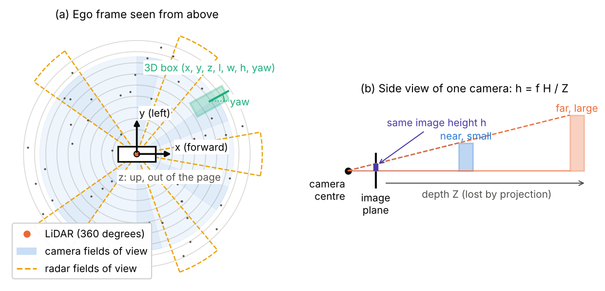
A convention used by the Waymo dataset, and by this chapter, is a right-handed vehicle frame with forward, to the left and up; each sensor has its own frame, and a 4×4 matrix called the extrinsics maps sensor coordinates into the vehicle frame [3]. In formulas, a point measured by a sensor becomes
where is a 3×3 rotation matrix and a 3-vector translation, together the sensor’s extrinsics. A camera additionally has intrinsics , a 3×3 matrix holding the focal lengths and the image centre in pixels. A point in camera coordinates (with pointing out of the lens) projects to the pixel
where are pixel coordinates. The division by is the heart of the matter: every point on the ray , , lands on the same pixel, so the depth is lost (Figure 1, right). Calibration matters in practice: if is off by half a degree, a point 60 m away moves by about half a metre, which is enough to paint a pedestrian’s pixels onto the wall behind them.
The bird’s-eye view
Plain version. BEV represents road scenes from above, making object size and position easier to compare in metric space. Vertical overlap remains possible.
In the BEV we drop and keep a 2D grid over , for example m cells. Height becomes a feature channel instead of an axis. Because objects keep their metric size and do not occlude each other in this view, an ordinary 2D convolutional detector can run on the BEV grid, and the planner downstream also thinks in this map. The price is that height detail is compressed, which matters little for cars on a road and more for indoor scenes with tables and shelves.
Point clouds: what the network actually sees
Plain version. Point clouds are unordered and spatially sparse. Distant objects usually receive fewer returns, so the representation must handle uneven sampling.
A LiDAR sweep is a set with , where is the intensity and is the number of points, often tens of thousands. Three properties shape every network in this chapter:
- Unordered. Any permutation of the list describes the same scene, so a network that consumes the points must be permutation invariant: for every permutation of the indices.
- Sparse. Points lie on surfaces. Divide the space around a car into 16 cm columns and more than 9 in 10 of them are empty (we measure this below).
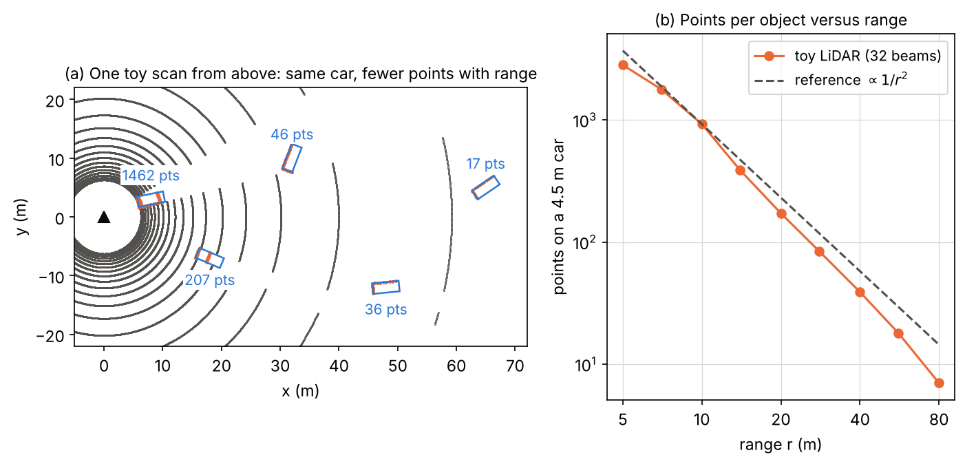
- Range-dependent density. A spinning LiDAR fires rays at fixed angular steps (horizontal) and (vertical). At range , neighbouring rays are about and apart, so an object of fixed face area receives about
points, where is the expected number of points and the angles are in radians. Doubling the distance cuts the points by about four.
The snippet below builds a toy spinning LiDAR (32 beams, one ray every 0.2 degrees) and counts the rays that hit a car-sized box placed at increasing range. It uses the slab method: a ray hits a box if the intervals where it lies between each pair of parallel faces overlap.
Code · Python · 26 lines
import numpy as np

# A toy spinning LiDAR mounted 1.8 m above the ground: 32 beams between -16 and +10 degrees
# elevation, one ray every 0.2 degrees of azimuth (1800 rays per beam per turn).
elev = np.deg2rad(np.linspace(-16, 10, 32))
azim = np.deg2rad(np.arange(0, 360, 0.2))
E, A = np.meshgrid(elev, azim, indexing="ij")
dirs = np.stack([np.cos(E) * np.cos(A), np.cos(E) * np.sin(A), np.sin(E)], -1).reshape(-1, 3)
origin = np.array([0.0, 0.0, 1.8])

def hits_on_box(center, size):
    """Count rays whose first hit is an axis-aligned box (slab method)."""
    lo, hi = center - size / 2, center + size / 2
    with np.errstate(divide="ignore", invalid="ignore"):
        t1, t2 = (lo - origin) / dirs, (hi - origin) / dirs
    t_near = np.nanmax(np.minimum(t1, t2), axis=1)
    t_far = np.nanmin(np.maximum(t1, t2), axis=1)
    return int(np.sum((t_far >= t_near) & (t_far > 0)))

car = np.array([4.5, 1.8, 1.5])                      # length, width, height in metres
ranges = np.array([5, 10, 20, 40, 80])
counts = np.array([hits_on_box(np.array([r, 0, car[2] / 2]), car) for r in ranges])
for r, c in zip(ranges, counts):
    print(f"car at {r:2d} m: {c:5d} points")
slope = np.polyfit(np.log(ranges[1:]), np.log(counts[1:]), 1)[0]
print(f"log-log slope (10-80 m): {slope:.2f}")
Output
car at  5 m:  2817 points
car at 10 m:   924 points
car at 20 m:   172 points
car at 40 m:    39 points
car at 80 m:     7 points
log-log slope (10-80 m): -2.33
The count drops from thousands of points at 5 m to 7 points at 80 m. The fitted slope is a bit steeper than because only a handful of the 32 beams cross a 1.5 m tall object far away, so the vertical sampling becomes coarse; real sensors with more beams follow more closely. Figure 2 shows the same effect on a whole scene: identical cars, very different evidence.
A classical baseline: ground removal, clustering and box fitting
Plain version. Before deep learning, a common LiDAR pipeline was: remove the road, group the remaining points into blobs, and draw a tight rectangle around each blob. It needs no training data, and it tells you exactly which problems the networks later had to solve.
The three steps are:
- Ground removal with RANSAC [5]. Fit a plane (unit normal , offset ) by repeatedly picking three random points, building the plane through them, and counting the inliers, points with for a tolerance . The plane with the most inliers is the ground. (RANSAC is explained in more detail in the Supplementary notes of IP 12 · Feature Extraction.)
- Clustering with DBSCAN [6]. Group the remaining points in the BEV: two points are neighbours if they are closer than , a point with at least neighbours is a core point, and clusters grow from core points; isolated points are labelled noise. DBSCAN needs no number of clusters, which suits a scene with an unknown number of objects. (See PR 07 · Clustering, Mixtures and EM for clustering in general.)
- Oriented box fitting. For each cluster, try yaw angles , rotate the points into the box frame, take the tight axis-aligned rectangle, and score it. Searching over angles with a fitting criterion is the idea of search-based L-shape fitting [7]. We use a simple criterion: the mean distance from each point to the nearest rectangle edge. A LiDAR usually sees an “L” (two sides of a car), and the right yaw puts those points on two edges.
Code · Python · 58 lines
import numpy as np
from sklearn.cluster import DBSCAN

rng = np.random.default_rng(0)

def box_surface(cx, cy, l, w, h, yaw, n):
    """n points on the sides of a yawed box that face the sensor at the origin."""
    c, s = np.cos(yaw), np.sin(yaw)
    pts = []
    for nx, ny, half, along in [(1, 0, l / 2, w), (-1, 0, l / 2, w), (0, 1, w / 2, l), (0, -1, w / 2, l)]:
        normal = np.array([c * nx - s * ny, s * nx + c * ny])
        mid = np.array([cx, cy]) + half * normal
        if normal @ mid >= 0:                      # face points away from the sensor: hidden
            continue
        t = rng.uniform(-along / 2, along / 2, n)
        tangent = np.array([-normal[1], normal[0]])
        xy = mid + t[:, None] * tangent
        pts.append(np.column_stack([xy, rng.uniform(0, h, n)]))
    return np.vstack(pts)

# ground plane z = 0 with slight noise, sampled uniformly in range and angle (density ~ 1/r)
r, a = rng.uniform(2, 60, 20000), rng.uniform(-np.pi / 2, np.pi / 2, 20000)
ground = np.column_stack([r * np.cos(a), r * np.sin(a), rng.normal(0, 0.03, r.size)])
objects = [(12, -4, 4.5, 1.8, 1.5, 0.3), (25, 6, 4.2, 1.7, 1.4, -1.0), (40, -10, 0.8, 0.6, 1.7, 0.0)]
cloud = [ground] + [box_surface(*o, n=int(40000 / np.hypot(o[0], o[1]) ** 2) + 5) for o in objects]
pts = np.vstack(cloud) + rng.normal(0, 0.02, (sum(len(c) for c in cloud), 3))

# 1) RANSAC plane fit: pick 3 points, count inliers within 0.1 m, keep the best plane
best = None
for _ in range(100):
    p = pts[rng.choice(len(pts), 3, replace=False)]
    n = np.cross(p[1] - p[0], p[2] - p[0])
    if np.linalg.norm(n) < 1e-9:
        continue
    n /= np.linalg.norm(n)
    inl = np.abs((pts - p[0]) @ n) < 0.1
    if best is None or inl.sum() > best.sum():
        best = inl
above = pts[~best]
print(f"{len(pts)} points, {best.sum()} ground inliers, {len(above)} left")

# 2) DBSCAN in the bird's-eye view
labels = DBSCAN(eps=0.7, min_samples=5).fit_predict(above[:, :2])

# 3) oriented box per cluster: search the yaw; score = mean distance of points to the nearest edge
for k in range(labels.max() + 1):
    q = above[labels == k]
    best_score, best_fit = np.inf, None
    for yaw in np.deg2rad(np.arange(0, 180, 1)):
        R = np.array([[np.cos(yaw), -np.sin(yaw)], [np.sin(yaw), np.cos(yaw)]])
        uv = q[:, :2] @ R                              # coordinates along the box axes
        lo, hi = uv.min(0), uv.max(0)
        edge_dist = np.minimum(np.minimum(uv - lo, hi - uv)[:, 0], np.minimum(uv - lo, hi - uv)[:, 1])
        if edge_dist.mean() < best_score and hi[0] - lo[0] >= hi[1] - lo[1]:   # x axis = long side
            best_score, best_fit = edge_dist.mean(), (R @ ((lo + hi) / 2), hi - lo, np.rad2deg(yaw))
    ctr, size, yaw = best_fit
    print(f"cluster {k}: {len(q):4d} pts, centre ({ctr[0]:5.1f}, {ctr[1]:5.1f}), "
          f"size {size[0]:.1f} x {size[1]:.1f} m, yaw {yaw:4.0f} deg, height {q[:, 2].max():.1f} m")
Output
20694 points, 19944 ground inliers, 750 left
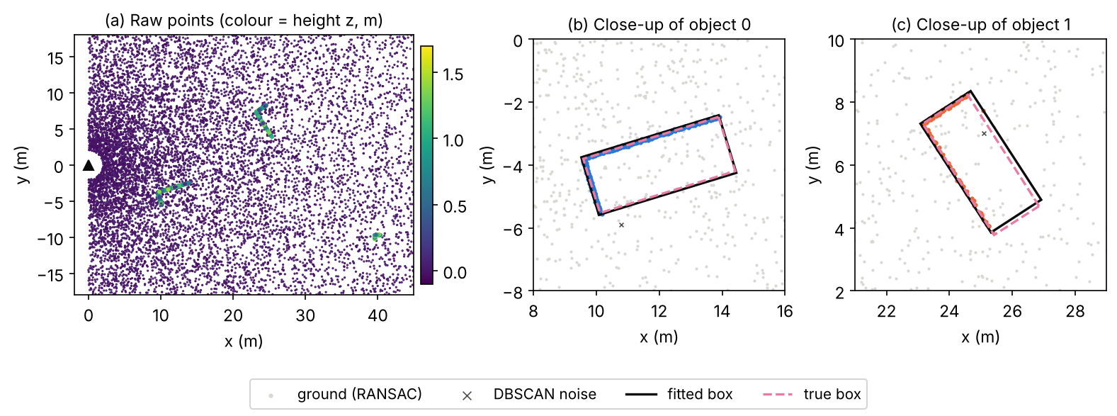
cluster 0:  471 pts, centre ( 12.0,  -4.0), size 4.6 x 1.9 m, yaw   17 deg, height 1.5 m
cluster 1:  124 pts, centre ( 25.0,   6.1), size 4.1 x 1.9 m, yaw  123 deg, height 1.4 m
cluster 2:   53 pts, centre ( 40.0,  -9.9), size 0.8 x 0.6 m, yaw    0 deg, height 1.7 m
On this synthetic scene (true objects: a car at with yaw 17°, a car at with yaw −57°, which is 123° modulo 180°, and a 0.8 × 0.6 m pedestrian at ) the pipeline recovers centres, sizes and yaws well. Figure 3 shows the result. A tempting simpler criterion, the smallest rectangle area, fails here: the hull of an L-shaped point set is roughly a triangle, and a rectangle along the triangle’s long diagonal encloses it with the same area, so the area criterion can pick a yaw about 20° off.
The baseline also shows its limits, and each one is a reason for learning:
- No semantics. A cluster is “something”. Telling a pedestrian from a pole, or a car from a bush, needs learned features.
- Partial views. The box is fitted to visible points only. A far car seen from the back gives a short line, so its length is unknown. Learned detectors use class-level size priors to complete what is not seen.
- Merging and splitting. Two people walking together merge into one cluster; a truck seen through a gap splits into two.
- Heading. The fit gives yaw only modulo 180°: it cannot tell the front of a car from its back.
3D boxes: encoding, IoU and NMS
These are the 3D versions of the building blocks of DLCV 03. We explain only what is new.
Box encoding and the yaw problem
Plain version. As in 2D, a network predicts small corrections to a reference box (an anchor or a point). The new part is the angle: angles wrap around, and a box turned by 180° covers exactly the same space, so a naive angle loss punishes the network for answers that are geometrically correct.
VoxelNet [8], SECOND [9] and PointPillars [10] use the same residuals between a ground-truth box (superscript ) and an anchor (superscript ):
where is the diagonal of the anchor’s base, which normalizes horizontal offsets in both directions by one length. These are the 2D targets of DLCV 03 with one more dimension.
For the angle, VoxelNet regressed the raw difference . SECOND [9] pointed out that this creates a conflict: a prediction off by exactly gives the same box but a large loss. Its sine-error loss
(with the predicted and the target angle, and SmoothL1 the smooth L1 loss of DLCV 03: quadratic for errors below 1, linear above) is zero both for a perfect prediction and for one flipped by . Because it cannot tell front from back, SECOND adds a small direction classifier with two bins that decides which way the box points [9]; PointPillars uses the same pair of losses [10]. CenterPoint instead regresses and recovers the angle with , which is continuous and unambiguous [11].
Optional: Yaw encodings compared (in the Supplementary notes). The four encodings side by side on worked angle pairs, including the flipped-box case.
BEV IoU and 3D IoU of rotated boxes
Plain version. IoU still means “overlap divided by total area”, but the boxes are now rotated, so the overlap is a polygon, not a rectangle. In 3D, multiply that polygon’s area by the overlap of the two height intervals.
For two upright boxes and , let be the intersection of their BEV rectangles (a convex polygon with up to 8 corners) and let
be the overlap of their vertical extents, where is a box’s centre height and its height. Then
where is area and are the box sizes. The intersection polygon of two convex polygons can be computed with Sutherland–Hodgman clipping [12]: cut the first polygon by each edge line of the second in turn, keeping only the part on the inner side. The polygon’s area then follows from the shoelace formula over its corners , with indices taken cyclically.
Code · Python · 58 lines
import numpy as np

def corners(box):
    """BEV corners (counter-clockwise) of box = (x, y, z, l, w, h, yaw); z is the box centre."""
    x, y, _, l, w, _, yaw = box
    c, s = np.cos(yaw), np.sin(yaw)
    local = np.array([[l, w], [-l, w], [-l, -w], [l, -w]]) / 2
    return local @ np.array([[c, s], [-s, c]]) + [x, y]

def clip(subject, clipper):
    """Sutherland-Hodgman: keep the part of polygon `subject` inside convex CCW polygon `clipper`."""
    out = list(subject)
    for i in range(len(clipper)):
        a, b = clipper[i], clipper[(i + 1) % len(clipper)]
        inside = lambda p: (b[0] - a[0]) * (p[1] - a[1]) - (b[1] - a[1]) * (p[0] - a[0]) >= 0
        pts, out = out, []
        for j in range(len(pts)):
            p, q = pts[j], pts[(j + 1) % len(pts)]
            if inside(q):
                if not inside(p):
                    out.append(cross_point(p, q, a, b))
                out.append(q)
            elif inside(p):
                out.append(cross_point(p, q, a, b))
        if not out:
            break
    return np.array(out)

def cross_point(p, q, a, b):
    """Intersection of segment p-q with the infinite line through a and b."""
    d1, d2 = q - p, b - a
    t = ((a[0] - p[0]) * d2[1] - (a[1] - p[1]) * d2[0]) / (d1[0] * d2[1] - d1[1] * d2[0])
    return p + t * d1

def area(poly):                                   # shoelace formula
    if len(poly) < 3:
        return 0.0
    x, y = poly[:, 0], poly[:, 1]
    return 0.5 * abs(x @ np.roll(y, -1) - y @ np.roll(x, -1))

def iou_bev_3d(a, b):
    inter = area(clip(corners(a), corners(b)))
    bev = inter / (a[3] * a[4] + b[3] * b[4] - inter)
    dz = max(0.0, min(a[2] + a[5] / 2, b[2] + b[5] / 2) - max(a[2] - a[5] / 2, b[2] - b[5] / 2))
    inter3 = inter * dz
    return bev, inter3 / (a[3] * a[4] * a[5] + b[3] * b[4] * b[5] - inter3)

car = (0, 0, 0, 4, 2, 1.5, 0)
cases = {"identical":                 (car, car),
         "rotated by 180 deg":        (car, (0, 0, 0, 4, 2, 1.5, np.pi)),
         "rotated by 90 deg":         (car, (0, 0, 0, 4, 2, 1.5, np.pi / 2)),
         "unit square vs 45 deg":     ((0, 0, 0, 1, 1, 1, 0), (0, 0, 0, 1, 1, 1, np.pi / 4)),
         "shifted 1 m along length":  (car, (1, 0, 0, 4, 2, 1.5, 0)),
         "same BEV, raised 0.5 m":    (car, (0, 0, 0.5, 4, 2, 1.5, 0)),
         "far apart":                 (car, (10, 0, 0, 4, 2, 1.5, 0.3))}
for name, (a, b) in cases.items():
    bev, iou3 = iou_bev_3d(np.array(a, float), np.array(b, float))
    print(f"{name:26s} BEV IoU {bev:.4f}   3D IoU {iou3:.4f}")
Output
identical                  BEV IoU 1.0000   3D IoU 1.0000
rotated by 180 deg         BEV IoU 1.0000   3D IoU 1.0000
rotated by 90 deg          BEV IoU 0.3333   3D IoU 0.3333
unit square vs 45 deg      BEV IoU 0.7071   3D IoU 0.7071
shifted 1 m along length   BEV IoU 0.6000   3D IoU 0.6000
same BEV, raised 0.5 m     BEV IoU 1.0000   3D IoU 0.5000
far apart                  BEV IoU 0.0000   3D IoU 0.0000
Every value matches a hand calculation: a 4 × 2 box against itself rotated by 90° overlaps in a 2 × 2 square, so ; a unit square against itself rotated by 45° overlaps in a regular octagon of area , which gives ; a box raised by a third of its height keeps the full BEV overlap but only half of the 3D one. Note the second line: a box turned by 180° has IoU 1. IoU is blind to the heading direction, which is why the Waymo metric adds a heading term (see below).
Figure 4 (right) shows how harsh yaw errors are for elongated objects. With a perfect centre and size, a car-sized box falls below IoU 0.7 at a yaw error of about 17°, and a bus-sized box at about 8.5°, while a square pedestrian box never drops below 0.7.
Rotated NMS and its alternatives
Plain version. Removing duplicate boxes works as in 2D, but “overlap” must now be measured between rotated boxes, which is slower. Two shortcuts are common: approximate the overlap with axis-aligned boxes, or avoid NMS altogether with centre peaks or set prediction.
Greedy NMS in 3D sorts boxes by score and removes those whose BEV IoU with a kept box exceeds a threshold, using the rotated IoU above. Because objects on a road rarely overlap in the BEV, the threshold can be low. PointPillars found that NMS on axis-aligned BEV boxes with threshold 0.5 gave similar results to rotated NMS and was much faster [10]. CenterPoint reads objects off the local maxima of a centre heatmap, like CenterNet [13], which removes most duplicates by construction; the paper still applies NMS to the peaks before its second stage [11]. Camera methods in the DETR family [14], such as DETR3D, predict a set of boxes and need no NMS at all [15].
LiDAR-based detectors
Plain version. LiDAR detectors differ mainly in how they turn an unordered point set into something a network can process: keep the points (point-based), drop them into a 3D grid (voxels), drop them into vertical columns (pillars), or mix the two. After that, most use a 2D detection head on the BEV.
Point-based: PointNet, PointNet++ and PointRCNN
Plain version. Process every point with the same small network, then summarize all points with a maximum. A maximum does not care about the order of its inputs, so the result is permutation invariant.
PointNet [16] computes
where is a shared multilayer perceptron applied to each point, is taken element-wise over the points (a symmetric function, so the order does not matter), and is a second network that maps the pooled feature to the output. It sees each point alone and then the whole set at once, so it misses local structure. PointNet++ [17] fixes this with set abstraction layers: choose a subset of centre points by farthest point sampling (each new centre is the point farthest from those already chosen), gather the neighbours within a radius of each centre (a ball query), and run a small PointNet on each neighbourhood. Stacking these layers gives a hierarchy of local features, like a CNN’s growing receptive fields. Both are mainly backbones: they produce features, and a detection head is built on top.
PointRCNN [18] is a two-stage detector that works directly on points. Stage 1 segments the scene into foreground and background points with a PointNet++ backbone and proposes a 3D box from each foreground point, bottom-up. Stage 2 pools the points inside each proposal, transforms them into the proposal’s own canonical coordinates (centred and rotated so the box is axis-aligned), and refines the box. Point-based detectors are accurate on small objects, but sampling and neighbour search on large clouds are slow.
Voxel-based: VoxelNet and SECOND
Plain version. Divide space into small 3D cells (voxels), summarize the points in each cell with a tiny PointNet, and then run convolutions on the resulting 3D grid. Because almost all voxels are empty, compute only where there are points.
VoxelNet [8] groups points by voxel and augments each point with its offset from the voxel’s centroid, giving a 7-D input , where is the mean of the points in the voxel. A stack of voxel feature encoding (VFE) layers, each a shared fully connected layer followed by element-wise max pooling within the voxel, turns each voxel into one feature vector. 3D convolutions then process the grid, and a region proposal network in the style of Faster R-CNN [19] predicts boxes on the BEV feature map. It was end-to-end and strong, but dense 3D convolutions made it slow.
SECOND [9] replaced the dense 3D convolutions by sparse convolutions, which store and compute only the occupied voxels. It uses mostly submanifold sparse convolutions [20], whose outputs are active only where the inputs are active, so the set of occupied sites does not grow layer after layer. SECOND also introduced the sine-error angle loss and ground-truth sampling augmentation (both described in this chapter), and sparse voxel backbones of this kind were adopted by later detectors such as PV-RCNN [21].
Optional: Sparse and submanifold convolution (in the Supplementary notes). Rule tables, why ordinary sparse convolution “dilates” the active set, and a small measurement.
Pillar-based: PointPillars
Plain version. Make the cells infinitely tall. Each vertical column (a pillar) is summarized by a tiny PointNet, and the result is a flat “pseudo-image” that an ordinary 2D CNN can process quickly.
PointPillars [10] has three stages: a pillar feature network, a 2D convolutional backbone and an SSD-style detection head [22]. Each point in a pillar is decorated to dimensions: , its offsets from the mean of the points in the pillar, and its offsets from the pillar’s centre in the – plane. The non-empty pillars are packed into a dense tensor of shape , with at most pillars per sample and points per pillar (12,000 and 100 in the paper, at a 0.16 m grid), zero-padded or randomly subsampled. A linear layer, batch normalization and ReLU are applied to every point, a max over the points gives one -dimensional feature per pillar, and the features are scattered back to their grid positions to form a pseudo-image. The paper reports 62 Hz for its full pipeline, and a faster variant at 105 Hz [10].
Optional: PointPillars: a reading guide (in the Paper guides). How to read the paper’s speed and accuracy tables, and what changed after KITTI switched to 40 recall positions.
The snippet performs the input side of this pipeline on a toy cloud: binning, the 9-D decoration, the dense tensor and the scatter (the PointNet weights are random here; in a real model they are learned).
Code · Python · 43 lines
import numpy as np

rng = np.random.default_rng(0)
# toy cloud: ground sampled uniformly in range and angle (so density falls as 1/r) + two "cars"
r, a = rng.uniform(2, 70, 10000), rng.uniform(-0.5, 0.5, 10000)
ground = np.column_stack([r * np.cos(a), r * np.sin(a), rng.normal(-1.7, 0.03, r.size)])
cars = [c + rng.uniform([-2.2, -0.9, -1.7], [2.2, 0.9, -0.2], (n, 3))
        for c, n in [(np.array([10.0, 2.0, 0.0]), 3000), (np.array([35.0, -6.0, 0.0]), 60)]]
xyz = np.vstack([ground] + cars)
pts = np.column_stack([xyz, rng.uniform(0, 1, len(xyz))])          # x, y, z, reflectance

# 1) bin into a bird's-eye-view grid of 0.16 m pillars over x in [0, 70.4), y in [-40, 40)
vx, x0, y0, W, H = 0.16, 0.0, -40.0, 440, 500
ix = np.floor((pts[:, 0] - x0) / vx).astype(int)
iy = np.floor((pts[:, 1] - y0) / vx).astype(int)
ok = (ix >= 0) & (ix < W) & (iy >= 0) & (iy < H)
pts, ix, iy = pts[ok], ix[ok], iy[ok]
pillar_id, inv, counts = np.unique(iy * W + ix, return_inverse=True, return_counts=True)
print(f"{len(pts)} points -> {len(pillar_id)} non-empty pillars out of {W * H} "
      f"({100 * (1 - len(pillar_id) / (W * H)):.1f}% empty); max {counts.max()} points in one pillar")

# 2) per-point 9-D features: x, y, z, r, offsets to the pillar mean, offsets to the pillar centre
mean = np.zeros((len(pillar_id), 3))
np.add.at(mean, inv, pts[:, :3])
mean /= counts[:, None]
centre = np.column_stack([(ix + 0.5) * vx + x0, (iy + 0.5) * vx + y0])
feat = np.column_stack([pts, pts[:, :3] - mean[inv], pts[:, :2] - centre])

# 3) dense tensor (P pillars, N points, D=9): pad with zeros, keep at most N points per pillar
P, N = len(pillar_id), 16          # PointPillars caps P at 12000 and N at 100, sampling at random
order = np.argsort(inv, kind="stable")
slot = np.arange(len(inv)) - np.searchsorted(inv[order], inv[order])   # rank inside its pillar
keep = slot < N
dense = np.zeros((P, N, 9))
dense[inv[order][keep], slot[keep]] = feat[order][keep]
print("dense pillar tensor:", dense.shape, "| points dropped by the cap N:", int((~keep).sum()))

# 4) a one-layer 'PointNet' (random weights here): linear + ReLU per point, max over points, scatter
Wt = rng.normal(0, 0.3, (9, 64))
pillar_feat = np.maximum(dense @ Wt, 0).max(axis=1)                      # (P, 64)
canvas = np.zeros((64, H * W))
canvas[:, pillar_id] = pillar_feat.T
print("pseudo-image:", canvas.reshape(64, H, W).shape)
Output
13060 points -> 9481 non-empty pillars out of 220000 (95.7% empty); max 24 points in one pillar
dense pillar tensor: (9481, 16, 9) | points dropped by the cap N: 23
pseudo-image: (64, 500, 440)
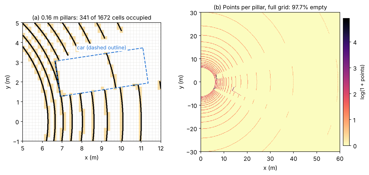
More than 95% of the 220,000 cells are empty in this toy, close to the roughly 97% sparsity the PointPillars paper reports for a real 64-beam sweep at the same grid size [10]. This is why pillarization and scattering, not the convolutions, decide how much memory the input step needs. Figure 5 shows the grid on a ray-cast scan.
Centre-based heads: CenterPoint
Plain version. Instead of anchors at several orientations, find object centres as peaks in a BEV heatmap and read every other property from the feature at the peak. A centre has no orientation, so the rotation problem of anchors disappears.
CenterPoint [11] keeps a standard voxel or pillar backbone and replaces the anchor head by a centre head in the spirit of CenterNet [13]. The heatmap has one channel per class and is trained with a focal loss [23] against Gaussian peaks rendered at the projected box centres; because objects are small in the BEV, the Gaussian radius is enlarged to at least 2 cells. At each centre, regression heads predict a sub-voxel offset, the height above ground, the 3D size, the yaw as and a 2D velocity. The velocity comes from feeding two consecutive sweeps, and it turns tracking into greedy closest-point matching of centres between frames. A light second stage samples features at the centres of the box faces and predicts a refined box and a confidence trained toward the box’s 3D IoU with the ground truth. Centre-based heads spread beyond LiDAR: the camera detector BEVDet, for example, uses CenterPoint’s head [24].
Point–voxel hybrids: PV-RCNN
Plain version. Voxels are fast and give good proposals; points keep exact positions. Use voxels to propose and points to refine.
PV-RCNN [21] runs a sparse 3D voxel CNN to get features and proposals, then summarizes the multi-scale voxel features into a small set of keypoints (voxel set abstraction). For each proposal, RoI-grid pooling gathers keypoint features at a regular grid of points inside the box, with several radii, and a refinement head predicts the final box and confidence. Two-stage hybrids of this kind were among the most accurate LiDAR detectors before transformer backbones.
Transformers and sequence models on points
Plain version. A car covers only a tiny part of a 150 m scene, so shrinking the feature map, as 2D networks do, throws away detail. Attention lets features interact over long distances without shrinking, if it is restricted to the occupied voxels.
SST [25] observed that downsampling brings little benefit in LiDAR detection and kept a single stride throughout, using attention among nearby occupied voxels to regain the receptive field that downsampling would have provided; the paper reports that this helps most on small objects such as pedestrians. DSVT [26] reorganized this attention so that it runs fully in parallel on a GPU and is easy to deploy. LION [27] and Voxel Mamba [28] replace attention by linear-time sequence models (a linear recurrent network and a state space model) that read the voxels as long sequences. The one thing to remember: these backbones buy long-range context at a cost that grows with the number of occupied voxels, not with the size of the scene.
Optional: Attention on sparse voxels (in the Supplementary notes). How windows, equal-size sets and space-filling-curve serialization make attention and sequence models practical on sparse voxels.
Camera-only 3D detection
Plain version. Cameras are cheap and see colour, texture and signs, but a photo is flat. Every camera detector must answer the same question: how far away is each thing it sees? This section first shows why that is hard, then the two main ways to build a 3D map from images: push pixels out into 3D, or pull image features into 3D positions.
Why one camera is not enough: depth ambiguity
Plain version. A photo of a toy car close up and a real car far away can look identical. To get depth from one image, a network must rely on clues such as the object’s typical size, where it touches the road and perspective, and small errors in those clues become large errors in metres far away.
For a pinhole camera with focal length (in pixels), an object of real height at depth appears pixels tall, so . Differentiating gives
so a one-pixel measurement error costs a depth error that grows with the square of the distance, and an error in the assumed size scales the depth by the same factor.
Code · Python · 9 lines
import numpy as np

f, H = 1000.0, 1.5                       # focal length in pixels, true car height in metres
for Z in [10, 20, 40, 80]:
    h = f * H / Z                        # image height of the car in pixels
    z_pix = f * H / (h - 1)              # depth if we mis-measure the height by one pixel
    z_size = f * (1.1 * H) / h           # depth if we assume a car 10% taller than it is
    print(f"Z = {Z:2d} m: car is {h:6.2f} px tall | 1 px error -> {z_pix - Z:5.2f} m | "
          f"10% size error -> {z_size - Z:4.1f} m")
Output
Z = 10 m: car is 150.00 px tall | 1 px error ->  0.07 m | 10% size error ->  1.0 m
Z = 20 m: car is  75.00 px tall | 1 px error ->  0.27 m | 10% size error ->  2.0 m
Z = 40 m: car is  37.50 px tall | 1 px error ->  1.10 m | 10% size error ->  4.0 m
Z = 80 m: car is  18.75 px tall | 1 px error ->  4.51 m | 10% size error ->  8.0 m
At 80 m a single pixel already moves the car by about 4.5 m, far outside a 3D IoU of 0.7. This is why monocular 3D detectors trail LiDAR so far on far objects. Monocular methods such as FCOS3D [29] adapt a 2D one-stage detector (FCOS [30]) to regress depth, size and orientation at the projected 3D centre. Pseudo-LiDAR [31] made an influential point: much of the gap between image-based and LiDAR-based detectors came from the representation, not only from depth quality; turning an estimated depth map into a 3D point cloud and running a LiDAR detector on it worked far better than processing the depth map as an image.
Lifting images into the bird’s-eye view
Plain version. Each pixel does not know its depth, so give it a probability distribution over depths, place a copy of its feature at every possible depth weighted by that probability, and then drop all those 3D features onto the BEV grid. The result can be fused across cameras and processed like a LiDAR BEV map.
Lift-Splat-Shoot (LSS) [32] “lifts” each image into a frustum of features. At each pixel, the network predicts a context vector and a distribution over a set of discrete depths (, ). The feature placed at depth along the pixel’s ray is
an outer product of depth probabilities and context. A confident depth puts the feature at one place; an uncertain depth spreads it along the ray. The “splat” step transforms all frustum points into the vehicle frame with the camera extrinsics and intrinsics and sum-pools them into BEV pillars, using a cumulative-sum trick to make the pooling fast [32]. The paper evaluated BEV segmentation and planning; BEVDet [24] turned the same view transform into a 3D detector with a BEV encoder and a centre-based head, plus data augmentation applied in both image and BEV space. BEVDepth [33] found that the depth distribution learned only from the detection loss was poor, and supervised it explicitly with depth from LiDAR points projected into the images, together with a depth network aware of the camera parameters.
Optional: Lift-Splat-Shoot: a reading guide (in the Paper guides). What the LSS paper actually evaluated, its robustness experiments and its limits.
Querying images from 3D: DETR3D, PETR and BEVFormer
Plain version. Go the other way round. Start from 3D guesses, either object queries or a grid of BEV cells, project them into the images with the known camera matrices, and fetch the image features they land on. No depth map is needed.
DETR3D [15] decodes each object query to a 3D reference point, projects it into all cameras, samples the image features there by bilinear interpolation and uses them to refine the query; training uses DETR’s set-to-set loss [14], so no NMS is needed. PETR [34] instead encodes 3D position into the image features themselves: the camera frustum is discretized into points at several depths, transformed to 3D with the camera parameters, and passed through a small network to produce a 3D position embedding that is added to the image features; ordinary DETR-style queries then attend to these position-aware features. BEVFormer [35] keeps a grid of learnable BEV queries, one per BEV cell. Spatial cross-attention lets each BEV query sample features in the image regions where its location projects, using deformable attention [36], and temporal self-attention lets it look at the BEV features of the previous frame, which helps with velocity and with objects that are briefly hidden. Its BEV map supports detection and map segmentation heads.
Time turned out to be a strong source of depth for cameras: motion between frames is a form of stereo. StreamPETR [37] propagates object queries from frame to frame online and reports camera-only results comparable to LiDAR-based methods on nuScenes, and Far3D [38] targets long-range camera detection with 3D queries generated from 2D detections.
Fusing LiDAR, cameras and radar
Plain version. LiDAR is good at “where”, cameras at “what”. Fusion combines them, and the main design question is where in the network to combine: at the raw points, at the proposals, in a shared BEV map, or through attention.
We group methods by where fusion happens; Wang et al. [39] give a finer taxonomy.
- Point-level (early) fusion. PointPainting [40] projects each LiDAR point into an image semantic segmentation and appends the class scores to the point; any LiDAR detector can then run on the “painted” cloud.
- Proposal-level fusion. MV3D [41] generates 3D proposals from a BEV map of the point cloud and fuses region features from the BEV, the LiDAR front view and the image. Frustum PointNets [42] go from 2D to 3D: a 2D detector finds the object in the image, and a PointNet processes only the points inside the frustum behind that 2D box.
- BEV-level fusion. Two methods named BEVFusion turn camera features into a BEV map (with an LSS-style view transform) and combine them with the LiDAR BEV map. One, from MIT [43], fuses with concatenation and a convolutional encoder, supports detection and map segmentation, and speeds up the camera-to-BEV pooling by more than 40 times. The other [44] keeps the camera stream independent of the LiDAR, so the detector still works when LiDAR fails, and reports large gains under simulated LiDAR malfunctions.
- Query-level fusion. TransFusion [45] first predicts object queries from LiDAR, then lets each query attend to image features with a transformer decoder. This “soft” association by attention, rather than a hard projection of points to pixels, makes it more robust to poor image conditions and calibration errors. UniTR [46] goes further and processes camera and LiDAR tokens with one shared transformer backbone.
Radar. Radar adds velocity and robustness to weather. CenterFusion [47] detects object centres in the image, associates radar returns with each detection through a frustum around it, and uses the radar features to improve depth, rotation and velocity, raising the nuScenes detection score of a camera detector substantially.
Training: assignment and augmentation
Plain version. Training a 3D detector resembles 2D training, with two twists: assignment uses rotated BEV overlaps or centre heatmaps, and data augmentation can cut objects out of one scene and paste them into another, which is impossible to do convincingly with photos.
Assignment. Anchor-based heads place a few anchors per BEV cell (one size per class, usually at yaw 0° and 90°) and assign them by BEV IoU, like the 2D rules of DLCV 03. VoxelNet’s car anchors, for instance, are positive above BEV IoU 0.6 and negative below 0.45 [8]. Because 3D scenes contain many more anchors than objects, these heads use the focal loss [23]. Centre-based heads replace IoU assignment by Gaussian heatmap targets [11].
Augmentation. LiDAR scenes are few (KITTI has 7,481 training scans [48]) and objects per scene are fewer still. Standard augmentations are [8], [9], [10]:
- Ground-truth sampling. Build a database of all labelled boxes and the points inside them, then paste randomly chosen objects into each training scene [9]. PointPillars samples 15 cars, 0 pedestrians and 8 cyclists per scene on KITTI [10]. VoxelNet already used a collision test to reject physically impossible results when perturbing boxes [8], and the same check is needed when pasting.
- Per-object perturbation. Rotate and translate each box with its points; VoxelNet draws rotations from and translations from a zero-mean Gaussian with standard deviation 1 m [8].
- Global transforms. Rotate the whole scene about the vertical axis (VoxelNet draws the angle from , simulating the car making a turn), scale it by a factor from , and flip it left–right [8], [10].
These are cheap because a point cloud is just coordinates: rotating points and boxes together keeps the labels exact. The catch is consistency across sensors: an object pasted into a LiDAR scan is not in the camera images, so fusion models need extra care.
Optional: Ground-truth sampling in detail (in the Supplementary notes). The database, the collision check and the pitfalls (floating objects, inconsistent occlusion, camera mismatch).
Datasets and metrics
Plain version. Three public benchmarks shaped the field. KITTI is small and front-facing, with a strict 3D IoU metric. nuScenes and Waymo are large and 360-degree; nuScenes matches boxes by centre distance and adds error terms, and Waymo weights each correct box by how well its heading matches.
| Dataset | Sensors (from the papers) | Scale (from the papers) | Main detection metric |
|---|---|---|---|
| KITTI 3D [49], [48] | Two stereo camera pairs (grey and colour), a Velodyne HDL-64E LiDAR | 7,481 training and 7,518 test images with point clouds; 80,256 labelled objects | 3D AP at IoU 0.7 (car) / 0.5 (pedestrian, cyclist), easy / moderate / hard |
| nuScenes [4], [50] | 6 cameras, 5 radars, 1 LiDAR, 360° | 1,000 scenes of 20 s; 23 classes and 8 attributes (10 classes for detection) | mAP with centre-distance matching; NDS |
| Waymo Open [3], [51] | 5 LiDARs, 5 cameras | 1,150 scenes of 20 s; about 12M labelled 3D LiDAR objects | mAPH at LEVEL_1 / LEVEL_2 |
KITTI: 3D AP with difficulty levels
On the KITTI 3D benchmark a detection is correct if its 3D IoU with a ground-truth box is at least 0.7 for cars and 0.5 for pedestrians and cyclists [48]. Objects are split into three cumulative difficulty levels by their image appearance [48]:
- Easy: 2D box at least 40 px tall, fully visible, at most 15% truncated.
- Moderate: at least 25 px tall, at most partly occluded, at most 30% truncated.
- Hard: at least 25 px tall, at most “difficult to see”, at most 50% truncated.
Methods are ranked by moderate AP. Since 8 October 2019 the benchmark computes AP from 40 recall positions instead of the original 11, following the analysis of Simonelli et al. [48], [52]; papers write this as , and numbers computed with the two rules must not be compared. The labels cover only objects visible in the front camera, so KITTI LiDAR detectors usually keep only the points that project into the image [10].
nuScenes: centre-distance mAP and NDS
Matching by distance. nuScenes does not use IoU to decide whether a detection is correct. A prediction matches the ground-truth object with the smallest 2D centre distance on the ground plane, if that distance is below a threshold [50]. AP is computed per class for thresholds m, integrating the precision–recall curve only where recall and precision exceed 0.1, and
where is the set of 10 detection classes and the set of distance thresholds in metres [50]. Each class is evaluated only within its own range from the ego vehicle (30 m for barriers and traffic cones, 40 m for bicycles, motorcycles and pedestrians, 50 m for the vehicle classes), and at most 500 boxes per sample may be submitted [50].
Why distance? IoU punishes the same centre error far more on small objects than on large ones (Figure 6). A 0.25 m error, for example, takes a 0.7 m pedestrian box to about IoU 0.47, below 0.5, while a car shifted by the same amount along its length keeps an IoU near 0.9.
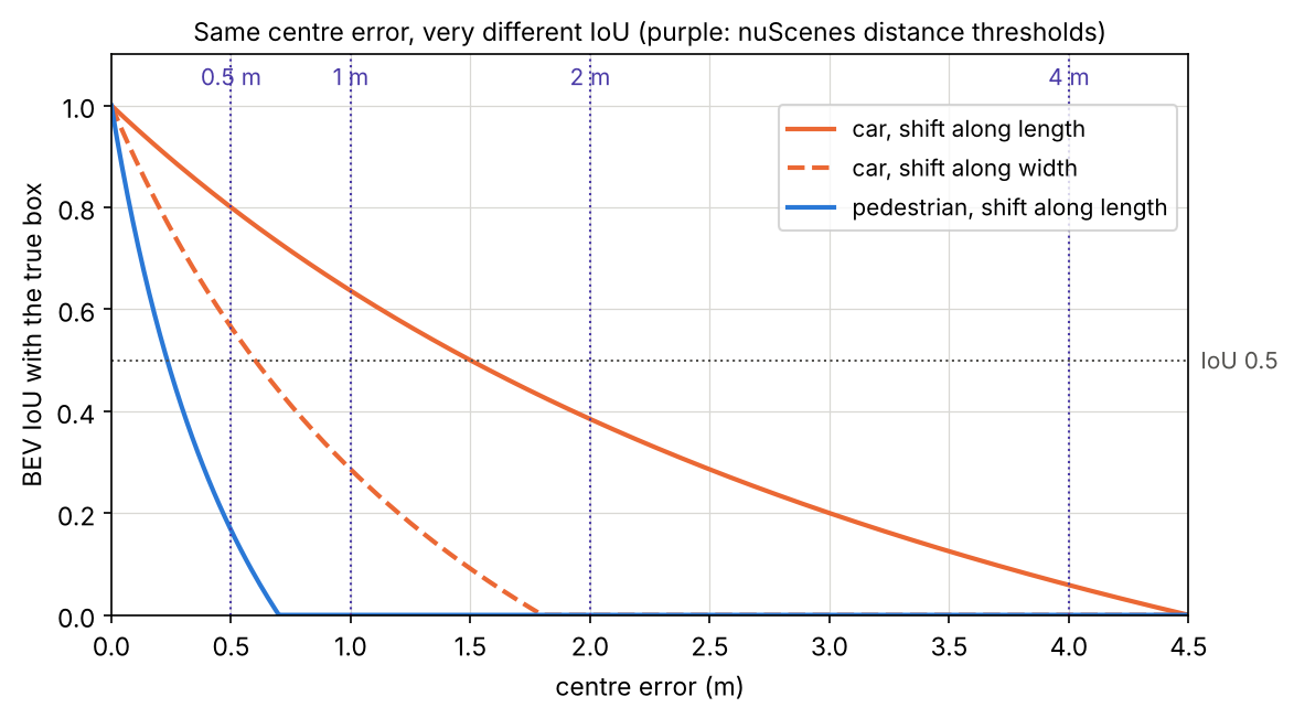
The snippet makes the same point with AP. Two classes get identical centre errors (Gaussian, standard deviation 0.25 m per axis) and the same number of false positives; only their sizes differ. (We compute plain 101-point interpolated AP and skip nuScenes’ 0.1 clipping, which does not change the comparison.)
Code · Python · 37 lines
import numpy as np

rng = np.random.default_rng(0)
size = {"car": (4.5, 1.8), "pedestrian": (0.7, 0.7)}     # BEV length x width in metres

def bev_iou(a, b):
    """Axis-aligned BEV IoU of boxes (x, y, l, w); yaw is 0 in this toy."""
    ox = max(0, min(a[0] + a[2] / 2, b[0] + b[2] / 2) - max(a[0] - a[2] / 2, b[0] - b[2] / 2))
    oy = max(0, min(a[1] + a[3] / 2, b[1] + b[3] / 2) - max(a[1] - a[3] / 2, b[1] - b[3] / 2))
    return ox * oy / (a[2] * a[3] + b[2] * b[3] - ox * oy)

def average_precision(gts, preds, is_match):
    """Greedy matching in score order; AP = mean interpolated precision at 101 recall points."""
    used, tp = np.zeros(len(gts), bool), []
    for p in sorted(preds, key=lambda p: -p[-1]):
        ok = [j for j in range(len(gts)) if not used[j] and is_match(p, gts[j])]
        if ok:
            j = min(ok, key=lambda j: np.hypot(p[0] - gts[j][0], p[1] - gts[j][1]))
            used[j] = True
        tp.append(bool(ok))
    tp = np.array(tp)
    recall = np.cumsum(tp) / len(gts)
    precision = np.cumsum(tp) / np.arange(1, len(tp) + 1)
    envelope = np.maximum.accumulate(precision[::-1])[::-1]
    return np.mean([envelope[recall >= r].max() if np.any(recall >= r) else 0
                    for r in np.linspace(0, 1, 101)])

for cls, (l, w) in size.items():
    gts = [(x, y, l, w) for x, y in rng.uniform(-50, 50, (100, 2))]
    preds = [(g[0] + dx, g[1] + dy, l, w, s) for g, (dx, dy), s in
             zip(gts, rng.normal(0, 0.25, (100, 2)), rng.uniform(0.3, 1, 100))]
    preds += [(x, y, l, w, s) for (x, y), s in zip(rng.uniform(-50, 50, (20, 2)), rng.uniform(0, 0.6, 20))]
    ap_iou = average_precision(gts, preds, lambda p, g: bev_iou(p, g) >= 0.5)
    ap_d = [average_precision(gts, preds, lambda p, g, t=t: np.hypot(p[0] - g[0], p[1] - g[1]) <= t)
            for t in (0.5, 1, 2, 4)]
    print(f"{cls:10s} AP(BEV IoU>=0.5) = {ap_iou:.3f} | AP(centre dist <= 0.5/1/2/4 m) = "
          f"{' / '.join(f'{a:.3f}' for a in ap_d)} | mean = {np.mean(ap_d):.3f}")
Output
car        AP(BEV IoU>=0.5) = 0.951 | AP(centre dist <= 0.5/1/2/4 m) = 0.789 / 0.988 / 0.988 / 0.990 | mean = 0.939
pedestrian AP(BEV IoU>=0.5) = 0.126 | AP(centre dist <= 0.5/1/2/4 m) = 0.791 / 0.979 / 0.979 / 0.979 | mean = 0.932
In this toy run, IoU matching rates the pedestrian detector as nearly useless (AP 0.126) and the car detector as excellent (0.951), although both made identical centre errors. Centre-distance matching gives both about the same score. Distance matching does not ignore box quality; it moves it into separate error terms.
True-positive errors and NDS. For matched detections at the 2 m threshold, nuScenes measures five TP errors: translation error ATE (centre distance in metres), scale error ASE ( after aligning centre and orientation), orientation error AOE (smallest yaw difference in radians), velocity error AVE (m/s) and attribute error AAE ( attribute accuracy) [50]. Their class means are combined with mAP into the nuScenes detection score:
where is the set of mean TP errors [50]. Half of NDS comes from mAP, the other half from box quality, orientation, velocity and attributes, which is why methods that estimate velocity well (with multiple sweeps or frames) gain a lot of NDS.
Optional: Computing NDS step by step (in the Supplementary notes). How TP errors are averaged, which classes skip which terms, and a worked comparison of two detectors.
Waymo: AP weighted by heading
The Waymo Open Dataset uses 3D IoU matching with thresholds 0.7 for vehicles and 0.5 for pedestrians and cyclists, and its primary metric is APH, average precision weighted by heading [51]. Each true positive counts not as 1 but as a heading accuracy
where and are the predicted and ground-truth headings in [3], [53]. A correct box facing exactly backwards () therefore counts as 0, which closes the loophole that IoU leaves open. Ground-truth boxes are split into two difficulty levels: LEVEL_2 for boxes with 1 to 5 LiDAR points (or marked as LEVEL_2 in the released labels), LEVEL_1 for the rest (boxes with no LiDAR points are not evaluated), and LEVEL_2 metrics include both [51]. Its 2020 3D detection challenge ranks entries by mAPH at LEVEL_2, the mean over vehicles, pedestrians and cyclists, and break results down by range: , and beyond 50 m [51].
Efficiency and deployment
Plain version. A car’s computer must finish perception well before the next sweep arrives, on embedded hardware, every time. The representation decides most of the cost: how many cells, how many points per cell, and whether the operators run fast on the target chip.
- Grid size and range set the budget. Halving the cell size quadruples the BEV cells. PointPillars traded accuracy for speed exactly this way, from 62 Hz at its default grid to 105 Hz with coarser pillars [10].
- Sparse operators need support. Sparse convolution and point sampling are efficient in principle, but they rely on custom kernels; pillar networks run on dense 2D convolutions that every inference engine supports. DSVT made deployment an explicit design goal, building its pooling without custom CUDA operators and reporting real-time inference after deployment [26].
- Camera view transforms are expensive. Lifting every pixel to many depths creates huge intermediate point sets; BEVFusion’s optimized BEV pooling reduced that step’s latency by more than 40 times [43].
- Benchmark speed is not vehicle speed. PointPillars’ paper notes that KITTI uses only the points inside the front camera’s view, about 10% of the sweep, and that timings on desktop GPUs do not transfer to embedded computers [10]. Measure end to end, on the target hardware, with full 360-degree input.
- Post-processing and temporal input count too. Rotated NMS runs over many boxes; multi-sweep inputs multiply the points. nuScenes limits the past sensor data a detection method may use to about 0.5 s [50].
Failure modes
Plain version. 3D detectors fail where the evidence is thin (far, small or hidden objects), where the sensors are disturbed (weather, dirt, miscalibration), and where the test data differ from the training data (another city, another sensor).
- Far and sparse objects. Points fall roughly with (Figure 2), so far objects have a few points or none. Benchmarks acknowledge this: Waymo assigns boxes with 1–5 points or an explicit difficulty flag to LEVEL_2, and its LEVEL_2 evaluation includes both difficulty levels [51]. nuScenes evaluates each class only within 30–50 m [50]. Camera depth errors grow with , which hurts the same objects.
- Occlusion and truncation. The sensor sees only surfaces facing it, and a parked car hides the pedestrian behind it. KITTI’s difficulty levels are defined by occlusion and truncation [48]; temporal models help by remembering briefly hidden objects [35].
- Confusable classes. PointPillars reports that pedestrians and cyclists are often confused with each other, and pedestrians with poles and tree trunks [10].
- Weather. Fog, rain and snow scatter laser pulses, creating spurious near returns and losing far ones. Hahner et al. simulate physically based fog on clear-weather LiDAR scans and show that training with it improves detection in real fog [54].
- Calibration and synchronization errors. Fusion that hard-projects points to pixels breaks when extrinsics drift; TransFusion’s soft association was designed for this [45], and LSS showed that training with noisy extrinsics or dropped cameras makes a camera BEV model more robust to them [32].
- Common corruptions. A benchmark of 27 LiDAR and camera corruptions applied to KITTI, nuScenes and Waymo, testing 24 detectors, found that motion-related corruptions hurt all models most, that LiDAR–camera fusion models were more robust, and that camera-only models were extremely vulnerable to image corruptions [55].
- Domain shift between datasets. A detector trained on one dataset can drop sharply on another. Wang et al. found that the main hurdle between German and US driving datasets was simply the different average car size, and that correcting for it closes much of the gap [56]. The Waymo paper itself reports a pronounced gap between data from different cities [3]. Different LiDAR models (beam count, mounting height) shift the point distribution too.
Modern view
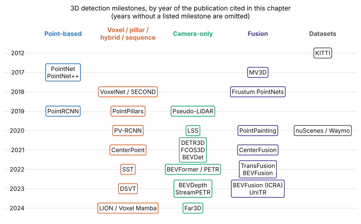
Figure 7 places the methods of this chapter on a timeline, by the year of each cited publication.
What the surveys say
Six surveys frame the field, each with its own taxonomy. Mao et al. [1] give the most complete map of 3D detection for driving: LiDAR methods by data representation (points, grids, point–voxel, range images), camera methods (monocular, stereo, multi-view), fusion, transformers, temporal and label-efficient detection, with an analysis of accuracy and speed trends. Qian et al. [2] cover sensors, datasets and metrics and include a case study with runtime, error and robustness analyses. Guo et al. [57] review deep learning on point clouds as a whole, of which detection is one task. For cameras, Ma et al. [58] and Li et al. [59] survey bird’s-eye-view perception; the latter frames the core problems as the view transformation, BEV ground truth, multi-sensor pipelines and generalization across sensor setups, and adds a practical “recipe” of tricks. Wang et al. [39] organize fusion methods by fusion stage, inputs and granularity. Two shared takeaways: the BEV has become the common meeting place of sensors and tasks, and accuracy gains on the standard benchmarks have outpaced gains in robustness and deployability.
Optional: Guide to the Modern view surveys (in the Paper guides). What each survey covers, how it organizes the field and how to use it.
The state of the art, 2023–2026
- LiDAR backbones have moved from sparse convolutions toward sparse transformers and linear-time sequence models over serialized voxels (DSVT [26], LION [27], Voxel Mamba [28]). Point Transformer V3 [60] argues that scale matters more than intricate design, and improves further with joint training on several datasets.
- Camera-only detection has narrowed the gap to LiDAR, mainly through temporal modelling and sparse queries (StreamPETR [37]) and better depth supervision (BEVDepth [33]); long-range camera detection is an active direction (Far3D [38]).
- Fusion in a shared BEV or token space (BEVFusion [43], [44], UniTR [46]) is the standard recipe for the strongest systems, and robustness to missing or degraded sensors is now a design goal rather than an afterthought.
- End-to-end driving. Detection is increasingly one stage of a single network trained for planning, as in UniAD [61], where perception, prediction and planning tasks communicate through unified query interfaces.
Open problems
- Far, small and rare objects. Sparse evidence at range, and classes that are rare in training data (animals, debris, unusual vehicles), remain weak points; closed-set datasets do not cover the long tail [1].
- Robustness. Weather, sensor faults, calibration drift and motion corruptions still cause large drops [55], [54].
- Generalization across sensors and places. Models trained on one LiDAR model, camera rig or city often fail on another [56], [3].
- Metrics that match driving. AP treats a missed pedestrian at 10 m and one at 45 m alike; nuScenes and Waymo add heading, velocity and range breakdowns, but, as Mao et al. note, maximizing AP alone may not be optimal for the driving system as a whole [1].
- Labels. 3D boxes are expensive to annotate, which motivates semi-supervised, self-supervised and auto-labelling methods [1].
Key takeaways
- State box conventions, units and coordinate transforms before interpreting detections.
- Point-cloud sparsity and range-dependent sampling shape the useful representations.
- BEV simplifies metric-space reasoning, but vertical structure and calibration still matter.
- Camera-only detection must infer depth; temporal and additional sensor evidence can help but introduce alignment requirements.
- Orientation errors can be hidden by overlap metrics; check yaw conventions and heading-sensitive measures.
- KITTI, nuScenes and Waymo use different matching and scoring rules; report the protocol and measure the deployed pipeline.
Exercises
- Points at range. A LiDAR has a horizontal step of 0.1° and a vertical step of 0.4°. Estimate how many points fall on the 1.8 m × 1.5 m back of a car at 20 m and at 60 m, using . How many beams cross the car vertically at 60 m?
Hint
Convert to radians: , . With m², and . Vertically, rays are m apart at 60 m, so only about 3–4 beams cross a 1.5 m tall object; the rest of the points come from the fine horizontal step.
- IoU by hand. Two 4 m × 2 m × 1.5 m boxes share a centre; one is rotated by 90° about the vertical axis. Compute the BEV IoU and the 3D IoU. Then raise the second box by 0.75 m and recompute the 3D IoU. Check your answers with the IoU snippet.
Hint
BEV intersection is a 2 m × 2 m square: . With equal heights the 3D IoU is also . Raised by 0.75 m, the height overlap is 0.75 m, so the intersection is 3 m³ and .
- Break the classical pipeline. In the classical-baseline snippet, move the pedestrian to , next to the first car (in our run its points come within about 0.15 m of the car’s points), and run it again. What does DBSCAN do? Change
epsto fix it, and explain what new failure a smallepscauses for the far objects.
Hint
In our run, every eps from 0.7 down to 0.15 merges the pedestrian and the car into one cluster with a wrong box (5.1 × 1.8 m at yaw 28° instead of 4.5 × 1.8 m at 17°). At eps=0.12 the pedestrian separates, but the car at 25 m already breaks into several fragments; at eps=0.1 even the near car splits into its two visible sides. Far objects have fewer points, so the gaps between their points are larger (on a real scanner they grow like ). A fixed eps cannot suit all ranges, a direct consequence of the density.
- Matching protocols. Using the matching snippet, find the standard deviation of the centre error at which the car’s AP under IoU ≥ 0.5 matches the pedestrian’s AP at standard deviation 0.25 m. What does this say about comparing per-class APs computed with IoU matching?
Hint
In our runs the car’s IoU-based AP falls to 0.117 at a standard deviation of 0.75 m, about three times the pedestrian’s 0.25 m (roughly the ratio of the car’s width to the pedestrian’s), in line with Figure 6. Per-class IoU-based APs therefore mix detection quality with object size, so a low pedestrian AP does not mean the pedestrian detector localizes worse in metres.
- Heading-weighted AP. A detector finds all 10 cars in a scene with no false positives and perfect IoU, but 3 of them face backwards and 2 are off by 30°. What are its AP and APH (assume all detections have the same score)? Which nuScenes TP error would reveal the same problem?
Hint
AP is 1, since every box matches. Heading accuracies: , so APH . In nuScenes the orientation error AOE (in radians) would rise, lowering NDS through the term .
- Pillar budget. In the pillarization snippet, change the grid to 0.32 m and to 0.08 m (adjust
WandHso the grid still covers 70.4 m × 80 m). Report the number of non-empty pillars, the share of empty cells and the number of points dropped by the cap . Relate the trend to the speed–accuracy trade-off reported by PointPillars.
Hint
In our runs, 0.32 m gives 7,567 non-empty pillars (86.2% empty) and drops 1,734 points at ; 0.08 m gives 10,908 pillars (98.8% empty) and drops none. Coarser pillars mean fewer, fuller pillars: a smaller pseudo-image and more points dropped by the cap, so faster but less precise. Finer pillars mean more pillars with one or two points each, a larger pseudo-image and more empty cells. PointPillars reports higher speed with coarser grids and a loss mainly for pedestrians and cyclists.
Detections are the input to tracking, which links them over time; see DLCV 07 · Object Tracking.
References
- J. Mao, S. Shi, X. Wang and H. Li, “3D object detection for autonomous driving: A comprehensive survey,” International Journal of Computer Vision, vol. 131, no. 8, 2023. doi
- R. Qian, X. Lai and X. Li, “3D object detection for autonomous driving: A survey,” Pattern Recognition, vol. 130, 2022. doi
- P. Sun, H. Kretzschmar, X. Dotiwalla, A. Chouard, V. Patnaik et al., “Scalability in perception for autonomous driving: Waymo Open Dataset,” in Proc. IEEE/CVF CVPR, 2020. CVF
- H. Caesar, V. Bankiti, A. H. Lang, S. Vora, V. E. Liong et al., “nuScenes: A multimodal dataset for autonomous driving,” in Proc. IEEE/CVF CVPR, 2020. CVF
- M. A. Fischler and R. C. Bolles, “Random sample consensus: A paradigm for model fitting with applications to image analysis and automated cartography,” Communications of the ACM, vol. 24, no. 6, 1981. doi
- M. Ester, H.-P. Kriegel, J. Sander and X. Xu, “A density-based algorithm for discovering clusters in large spatial databases with noise,” in Proc. KDD, 1996. AAAI
- X. Zhang, W. Xu, C. Dong and J. M. Dolan, “Efficient L-shape fitting for vehicle detection using laser scanners,” in Proc. IEEE Intelligent Vehicles Symposium (IV), 2017. doi
- Y. Zhou and O. Tuzel, “VoxelNet: End-to-end learning for point cloud based 3D object detection,” in Proc. IEEE CVPR, 2018. CVF
- Y. Yan, Y. Mao and B. Li, “SECOND: Sparsely embedded convolutional detection,” Sensors, vol. 18, no. 10, 3337, 2018. doi
- A. H. Lang, S. Vora, H. Caesar, L. Zhou, J. Yang and O. Beijbom, “PointPillars: Fast encoders for object detection from point clouds,” in Proc. IEEE/CVF CVPR, 2019. CVF
- T. Yin, X. Zhou and P. Krähenbühl, “Center-based 3D object detection and tracking,” in Proc. IEEE/CVF CVPR, 2021. CVF
- I. E. Sutherland and G. W. Hodgman, “Reentrant polygon clipping,” Communications of the ACM, vol. 17, no. 1, 1974. doi
- X. Zhou, D. Wang and P. Krähenbühl, “Objects as points,” arXiv:1904.07850, 2019. arXiv
- N. Carion, F. Massa, G. Synnaeve, N. Usunier, A. Kirillov and S. Zagoruyko, “End-to-end object detection with transformers,” in Proc. ECCV, 2020. doi
- Y. Wang, V. Guizilini, T. Zhang, Y. Wang, H. Zhao and J. Solomon, “DETR3D: 3D object detection from multi-view images via 3D-to-2D queries,” in Proc. Conference on Robot Learning (CoRL), 2021. arXiv
- C. R. Qi, H. Su, K. Mo and L. J. Guibas, “PointNet: Deep learning on point sets for 3D classification and segmentation,” in Proc. IEEE CVPR, 2017. arXiv
- C. R. Qi, L. Yi, H. Su and L. J. Guibas, “PointNet++: Deep hierarchical feature learning on point sets in a metric space,” in Advances in Neural Information Processing Systems (NeurIPS), 2017. NeurIPS
- S. Shi, X. Wang and H. Li, “PointRCNN: 3D object proposal generation and detection from point cloud,” in Proc. IEEE/CVF CVPR, 2019. arXiv
- S. Ren, K. He, R. Girshick and J. Sun, “Faster R-CNN: Towards real-time object detection with region proposal networks,” IEEE TPAMI, vol. 39, no. 6, 2017. doi
- B. Graham, M. Engelcke and L. van der Maaten, “3D semantic segmentation with submanifold sparse convolutional networks,” in Proc. IEEE CVPR, 2018. CVF
- S. Shi, C. Guo, L. Jiang, Z. Wang, J. Shi, X. Wang and H. Li, “PV-RCNN: Point-voxel feature set abstraction for 3D object detection,” in Proc. IEEE/CVF CVPR, 2020. arXiv
- W. Liu, D. Anguelov, D. Erhan, C. Szegedy, S. Reed, C.-Y. Fu and A. C. Berg, “SSD: Single shot multibox detector,” in Proc. ECCV, 2016. arXiv
- T.-Y. Lin, P. Goyal, R. Girshick, K. He and P. Dollár, “Focal loss for dense object detection,” in Proc. IEEE ICCV, 2017. doi
- J. Huang, G. Huang, Z. Zhu, Y. Ye and D. Du, “BEVDet: High-performance multi-camera 3D object detection in bird-eye-view,” arXiv:2112.11790, 2021. arXiv
- L. Fan, Z. Pang, T. Zhang, Y.-X. Wang, H. Zhao, F. Wang, N. Wang and Z. Zhang, “Embracing single stride 3D object detector with sparse transformer,” in Proc. IEEE/CVF CVPR, 2022. CVF
- H. Wang, C. Shi, S. Shi, M. Lei, S. Wang, D. He, B. Schiele and L. Wang, “DSVT: Dynamic sparse voxel transformer with rotated sets,” in Proc. IEEE/CVF CVPR, 2023. CVF
- Z. Liu, J. Hou, X. Wang, X. Ye, J. Wang, H. Zhao and X. Bai, “LION: Linear group RNN for 3D object detection in point clouds,” in Advances in Neural Information Processing Systems (NeurIPS), 2024. NeurIPS
- G. Zhang, L. Fan, C. He, Z. Lei, Z. Zhang and L. Zhang, “Voxel Mamba: Group-free state space models for point cloud based 3D object detection,” in Advances in Neural Information Processing Systems (NeurIPS), 2024. NeurIPS
- T. Wang, X. Zhu, J. Pang and D. Lin, “FCOS3D: Fully convolutional one-stage monocular 3D object detection,” in Proc. IEEE/CVF ICCV Workshops, 2021. arXiv
- Z. Tian, C. Shen, H. Chen and T. He, “FCOS: Fully convolutional one-stage object detection,” in Proc. IEEE/CVF ICCV, 2019. arXiv
- Y. Wang, W.-L. Chao, D. Garg, B. Hariharan, M. Campbell and K. Q. Weinberger, “Pseudo-LiDAR from visual depth estimation: Bridging the gap in 3D object detection for autonomous driving,” in Proc. IEEE/CVF CVPR, 2019. arXiv
- J. Philion and S. Fidler, “Lift, splat, shoot: Encoding images from arbitrary camera rigs by implicitly unprojecting to 3D,” in Proc. ECCV, 2020. arXiv
- Y. Li, Z. Ge, G. Yu, J. Yang, Z. Wang, Y. Shi, J. Sun and Z. Li, “BEVDepth: Acquisition of reliable depth for multi-view 3D object detection,” in Proc. AAAI, 2023. arXiv
- Y. Liu, T. Wang, X. Zhang and J. Sun, “PETR: Position embedding transformation for multi-view 3D object detection,” in Proc. ECCV, 2022. arXiv
- Z. Li, W. Wang, H. Li, E. Xie, C. Sima, T. Lu, Y. Qiao and J. Dai, “BEVFormer: Learning bird’s-eye-view representation from multi-camera images via spatiotemporal transformers,” in Proc. ECCV, 2022. arXiv
- X. Zhu, W. Su, L. Lu, B. Li, X. Wang and J. Dai, “Deformable DETR: Deformable transformers for end-to-end object detection,” in Proc. ICLR, 2021. arXiv
- S. Wang, Y. Liu, T. Wang, Y. Li and X. Zhang, “Exploring object-centric temporal modeling for efficient multi-view 3D object detection,” in Proc. IEEE/CVF ICCV, 2023. CVF
- X. Jiang, S. Li, Y. Liu, S. Wang, F. Jia, T. Wang, L. Han and X. Zhang, “Far3D: Expanding the horizon for surround-view 3D object detection,” in Proc. AAAI, 2024. arXiv
- Y. Wang, Q. Mao, H. Zhu, J. Deng, Y. Zhang, J. Ji, H. Li and Y. Zhang, “Multi-modal 3D object detection in autonomous driving: A survey,” International Journal of Computer Vision, vol. 131, no. 8, 2023. doi
- S. Vora, A. H. Lang, B. Helou and O. Beijbom, “PointPainting: Sequential fusion for 3D object detection,” in Proc. IEEE/CVF CVPR, 2020. arXiv
- X. Chen, H. Ma, J. Wan, B. Li and T. Xia, “Multi-view 3D object detection network for autonomous driving,” in Proc. IEEE CVPR, 2017. arXiv
- C. R. Qi, W. Liu, C. Wu, H. Su and L. J. Guibas, “Frustum PointNets for 3D object detection from RGB-D data,” in Proc. IEEE CVPR, 2018. CVF
- Z. Liu, H. Tang, A. Amini, X. Yang, H. Mao, D. Rus and S. Han, “BEVFusion: Multi-task multi-sensor fusion with unified bird’s-eye view representation,” in Proc. IEEE ICRA, 2023. arXiv
- T. Liang, H. Xie, K. Yu, Z. Xia, Z. Lin, Y. Wang, T. Tang, B. Wang et al., “BEVFusion: A simple and robust LiDAR-camera fusion framework,” in Advances in Neural Information Processing Systems (NeurIPS), 2022. arXiv
- X. Bai, Z. Hu, X. Zhu, Q. Huang, Y. Chen, H. Fu and C.-L. Tai, “TransFusion: Robust LiDAR-camera fusion for 3D object detection with transformers,” in Proc. IEEE/CVF CVPR, 2022. arXiv
- H. Wang, H. Tang, S. Shi, A. Li, Z. Li, B. Schiele and L. Wang, “UniTR: A unified and efficient multi-modal transformer for bird’s-eye-view representation,” in Proc. IEEE/CVF ICCV, 2023. arXiv
- R. Nabati and H. Qi, “CenterFusion: Center-based radar and camera fusion for 3D object detection,” in Proc. IEEE/CVF WACV, 2021. doi
- A. Geiger, P. Lenz, C. Stiller and R. Urtasun, “3D object detection evaluation 2017,” The KITTI Vision Benchmark Suite, official benchmark page (data sizes, IoU thresholds, difficulty levels, 40 recall positions). link
- A. Geiger, P. Lenz and R. Urtasun, “Are we ready for autonomous driving? The KITTI vision benchmark suite,” in Proc. IEEE CVPR, 2012. doi
- nuScenes devkit, “nuScenes detection task,” official evaluation documentation (classes, detection ranges, mAP, TP metrics, NDS, submission rules). link
- Waymo Open Dataset, “3D detection challenge (2020),” official challenge page (APH, IoU thresholds, LEVEL_1/LEVEL_2, range breakdown). link
- A. Simonelli, S. Rota Bulò, L. Porzi, M. López-Antequera and P. Kontschieder, “Disentangling monocular 3D object detection,” in Proc. IEEE/CVF ICCV, 2019. doi
- Waymo Open Dataset,
metrics_utils.cc, official metric implementation (functionComputeHeadingAccuracy). code - M. Hahner, C. Sakaridis, D. Dai and L. Van Gool, “Fog simulation on real LiDAR point clouds for 3D object detection in adverse weather,” in Proc. IEEE/CVF ICCV, 2021. arXiv
- Y. Dong, C. Kang, J. Zhang, Z. Zhu, Y. Wang, X. Yang, H. Su, X. Wei et al., “Benchmarking robustness of 3D object detection to common corruptions in autonomous driving,” in Proc. IEEE/CVF CVPR, 2023. arXiv
- Y. Wang, X. Chen, Y. You, L. E. Li, B. Hariharan, M. Campbell, K. Q. Weinberger and W.-L. Chao, “Train in Germany, test in the USA: Making 3D object detectors generalize,” in Proc. IEEE/CVF CVPR, 2020. arXiv
- Y. Guo, H. Wang, Q. Hu, H. Liu, L. Liu and M. Bennamoun, “Deep learning for 3D point clouds: A survey,” IEEE TPAMI, vol. 43, no. 12, 2021. doi
- Y. Ma, T. Wang, X. Bai, H. Yang, Y. Hou, Y. Wang, Y. Qiao, R. Yang and X. Zhu, “Vision-centric BEV perception: A survey,” IEEE TPAMI, vol. 46, no. 12, 2024. doi
- H. Li, C. Sima, J. Dai, W. Wang, L. Lu, H. Wang, J. Zeng, Z. Li et al., “Delving into the devils of bird’s-eye-view perception: A review, evaluation and recipe,” IEEE TPAMI, vol. 46, no. 4, 2024. doi
- X. Wu, L. Jiang, P.-S. Wang, Z. Liu, X. Liu, Y. Qiao, W. Ouyang, T. He and H. Zhao, “Point Transformer V3: Simpler, faster, stronger,” in Proc. IEEE/CVF CVPR, 2024. arXiv
- Y. Hu, J. Yang, L. Chen, K. Li, C. Sima, X. Zhu, S. Chai, S. Du et al., “Planning-oriented autonomous driving,” in Proc. IEEE/CVF CVPR, 2023. arXiv
Check your understanding
This tutorial has 6 exercises. Can you solve them without opening the hints?
Go to the exercises ↑Next DLCV 04 · Image Segmentation: Semantic, Instance and Panoptic · 37 min