DLCV 12 · Image Generation: From GANs to Text-to-Image Systems
Needs: ML 07 · Generative Models: Autoencoders, VAEs, GANs and Flows, ML 08 · Diffusion Models and Flow Matching
Navigate: this page and this track: Navigate: this page and this track
On this page
- What you’ll learn1 min
- The big picture2 min
- The task: what to generate, and what “good” means2 min
- The model families on one map3 min
- The text-to-image system7 min
- Control, personalization and editing3 min
- Autoregressive and unified multimodal generators4 min
- Evaluating text-to-image models5 min
- Data1 min
- Risks and responsible use2 min
- Failure modes1 min
- Modern view2 min
- Key takeaways1 min
- Exercises3 min
- Supplementary notes
- Paper guides
- References
Deep Learning for Computer Vision
What you’ll learn
- Define generation and editing tasks through their conditions and required outputs.
- Distinguish generator families from pixel, latent and token representations.
- Trace text encoding, conditioning, sampling and decoding.
- Compare spatial control, personalization and editing mechanisms.
- Evaluate quality, diversity, alignment, cost and data-related failure modes.
The big picture
An image generator turns a request into a new picture. The request can be nothing at all (“any face”), a class label (“a goldfinch”), a sentence (“a red ball on the grass”), or another image plus an instruction (“make it winter”). The answer should look real, should vary from one try to the next, and should actually show what was asked.
Why it matters. Image generation went from small, blurry faces to photorealistic, prompt-following pictures in less than a decade, and it is now part of design tools, photo editors, data pipelines and restoration systems (DLCV 09B uses the same models to restore damaged photos). As a computer-vision system, a modern generator combines a language model, an image compressor, a generative network, a sampler and an evaluation pipeline. Each part can fail on its own, and each part has its own literature.
Where this chapter sits. The theory lives in the ML track, and this chapter does not repeat it. ML 07 derives VAEs, GANs, normalizing flows and the classic metrics (Inception Score, FID, precision and recall) with code. ML 08 derives diffusion, DDIM, classifier-free guidance, latent diffusion, diffusion transformers, flow matching and few-step samplers. ML 09 covers autoregressive models over pixels and tokens, and ML 10 covers CLIP and parameter-efficient fine-tuning. Here we take the system view: how these pieces are assembled into text-to-image products, how they are steered, how they are judged, and what can go wrong. The two code examples run in seconds on a CPU with NumPy and scikit-image, and use no network weights.
Next. DLCV 12A extends these systems from images to video.
The task: what to generate, and what “good” means
Plain version. Generation produces outputs under conditions such as text, labels or an input image. Evaluate realism, diversity and adherence to those conditions separately.
Six kinds of generation
All the tasks below are sampling from a conditional distribution , where is an image and is the condition; the unconditional case uses an empty condition .
| Task | Condition | Output | Example method in this chapter |
|---|---|---|---|
| Unconditional | nothing | an image from the training domain | StyleGAN on faces [1] |
| Class-conditional | a class label | an image of that class | BigGAN [2], DiT [3] |
| Text-to-image | a text prompt | an image matching the prompt | Imagen [4], latent diffusion [5] |
| Image-to-image | an image (often plus text) | a new image that keeps its structure | SDEdit [6], ControlNet [7] |
| Editing | an image plus an edit request | the edited image | Prompt-to-Prompt [8], InstructPix2Pix [9] |
| Inpainting / outpainting | an image plus a mask | the image with the masked region filled | RePaint [10] |
Because the form is shared, one trained text-to-image model can serve most rows of the table: edits, masks and control images are extra conditions or a different starting point for the sampler.
Three questions: fidelity, diversity, alignment
- Fidelity (quality). Does each sample look like a real image of the domain, without artifacts?
- Diversity (coverage). Do many samples together cover the variety of real images, or does the model repeat a few favorites (mode collapse)?
- Alignment. Does the sample show what the condition asked for: the right objects, counts, colors, positions and text?
Add a fourth, practical question: cost, the number of network evaluations and the seconds per image. The first three questions pull against each other. Most generators expose a dial that trades diversity for fidelity and alignment: the truncation trick of BigGAN shrinks the spread of the input noise [2], and classifier-free guidance in diffusion models pushes samples toward the condition [11]. Turning such a dial up makes images cleaner and more on-prompt, but more alike. Keep this trade-off in mind whenever you read a single “quality” number. The metrics that measure fidelity and diversity separately are derived in ML 07; this chapter adds the alignment side in the evaluation section below.
The model families on one map
Plain version. GANs, diffusion, flow and autoregressive models learn different generation procedures. Separately choose whether the system represents images as pixels, continuous latents or tokens.
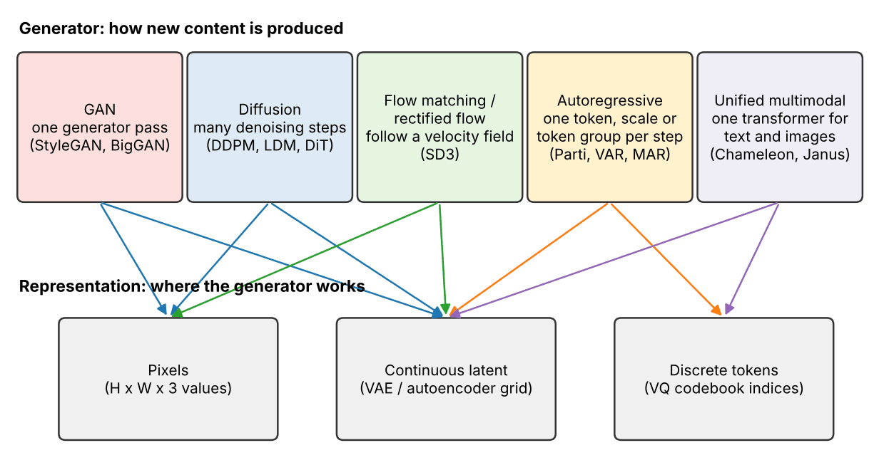
GANs: one pass through a generator. A generator maps random noise to an image, and a discriminator, trained at the same time, tries to tell generated images from real ones; the generator improves by fooling it [12]. Sampling is a single forward pass, so GANs are fast. StyleGAN [1] maps the noise to an intermediate “style” vector and injects it at every resolution of the generator, which separates coarse attributes (pose, identity) from fine ones (freckles, hair) and allows scale-specific control. BigGAN [2] scaled class-conditional GANs on ImageNet and introduced the truncation trick mentioned above. Training is unstable and can miss modes, which made GANs hard to scale to open-ended prompts. Theory and code: ML 07, GANs.
VAEs and tokenizers: compress first. A variational autoencoder (VAE) learns an encoder to a compact latent code, a decoder back to pixels, and a simple prior over codes [13]. In today’s systems the autoencoder’s main job is compression in front of another generator: latent diffusion runs its denoiser on a continuous latent grid that is several times smaller than the image [5], and token-based models use a vector-quantized autoencoder (VQ-VAE [14], VQGAN [15]) that turns an image into a grid of integer indices from a learned codebook, like words from a dictionary. The decoder sets a ceiling: no generator can produce detail the decoder cannot reconstruct. Details: ML 07, VAEs and ML 09, visual tokens.
Diffusion: many small denoising steps. Train a network to remove a little Gaussian noise from a noisy image; to generate, start from pure noise and apply it many times [16]. Training is a stable regression, and with better architectures and classifier guidance diffusion models overtook GANs on ImageNet [17]. Running the same process on an autoencoder’s latent grid, latent diffusion, made high-resolution text-to-image generation affordable [5]. Theory and code: ML 08 and its section on latent diffusion.
Flow matching and rectified flow: follow a velocity field. Draw a noise sample and a data sample, connect them with a straight line, and train a network to predict the direction of travel along such lines; to generate, start from noise and follow the predicted directions [18], [19]. It is closely related to diffusion (a different path between noise and data) and is now used at scale: Stable Diffusion 3 trains a large latent transformer with a rectified-flow objective [20]. Theory: ML 08, flow matching.
Autoregressive and unified models: write the picture piece by piece. Turn the image into a sequence of tokens and predict the next token (or the next group of tokens, or the next, sharper version of the whole token map) given everything generated so far. This is the language-model recipe applied to images, and its newest form is a single transformer that reads and writes both text and images. It gets its own section below.
| Family | How it samples | Sequential network calls | Main strength | Main thing to watch |
|---|---|---|---|---|
| GAN | one generator pass | one | speed, smooth editable latent space | training stability, mode coverage |
| Diffusion | repeated denoising from noise | tens to hundreds; fewer with distillation | quality, coverage, stable training | sampling cost |
| Flow matching | integrate a learned velocity | tens; fewer with distillation | simple objective, straighter paths | still needs several steps unless distilled |
| Autoregressive | predict tokens in some order | one per token, group or scale | reuses language-model machinery, exact likelihood of tokens | tokenizer ceiling, error accumulation |
Two points from the map are easy to forget. The generator and the representation are separate choices: a diffusion model can work on pixels (Imagen [4]) or on latents (latent diffusion [5]), and an autoregressive model can use discrete or continuous tokens [21]. And real systems mix families: an adversarial loss trains the tokenizer of VQGAN [15], and adversarial distillation turns a diffusion model into a one-to-four-step generator [22].
The text-to-image system
Plain version. A latent text-to-image pipeline encodes the prompt, generates a conditioned latent representation and decodes pixels. The conditioning interface connects language to image features.
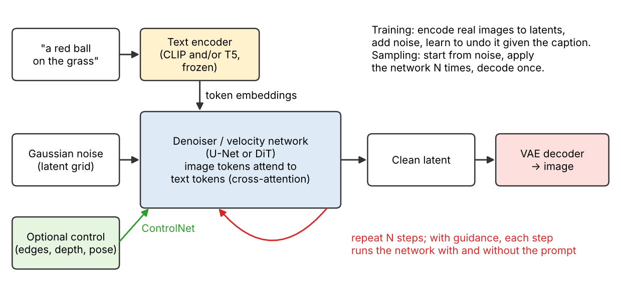
In training, each image of an image–caption pair is encoded to a latent, noised to a random level, and the denoiser learns to undo the noise given the caption’s embeddings. At sampling time, the denoiser starts from pure noise and runs for steps, then the decoder produces pixels. The diffusion and sampling equations behind these two sentences are in ML 08; below we look at the parts that are specific to text.
Text encoders: CLIP or a language model
Plain version. The text encoder decides what the generator can “understand”. A model trained to match images and captions knows visual concepts; a large language model trained on text alone knows grammar, word order and spelling-related structure better. Many systems use both.
Two kinds of encoder dominate:
- CLIP text encoders are trained contrastively so that an image and its caption land near each other in a shared embedding space [23] (see ML 10). Their embeddings are visually grounded.
- Language-model encoders such as T5 [24] are trained on text only. Imagen’s key finding was that a large frozen T5 encoder works surprisingly well, and that making the text encoder larger improved both fidelity and image–text alignment much more than making the image diffusion model larger [4].
Recent systems combine them. SDXL adds a second text encoder to the design of earlier Stable Diffusion models [25]. Stable Diffusion 3 uses three frozen encoders, two CLIP models and T5-XXL; its authors report that dropping T5 at inference time costs little on most prompts but clearly hurts prompts with long written text or many details [20]. A related finding concerns spelling: text encoders that see whole word pieces rather than characters (“character-blind”) make it hard to draw a word letter by letter, and character-aware encoders render visual text much more accurately [26]. DALL·E 2 takes yet another route: a “prior” network first generates a CLIP image embedding from the caption, and a diffusion decoder then generates the image from that embedding [27].
Cross-attention: how words reach pixels
Plain version. At every layer, each position of the image asks a question (“what should be here?”) and looks over all the words of the prompt to find the ones that answer it. The answer it collects is a weighted mix of the words, with large weights on the words that match.
Latent diffusion introduced cross-attention layers into the U-Net denoiser for this purpose [5]. Let be the image features at one layer ( spatial positions, each a vector of width ), and the text-encoder outputs ( tokens of width ). Learned matrices , project them to a common width :
Here holds one query per image position, hold one key and one value per text token, the softmax is taken along each row, and is the attention map: row is a probability distribution over the tokens that says how much position listens to each word. The output gives every image position a mix of word values; it is added back to the image features. Queries come from the image and keys and values come from the text, which is exactly what makes it cross-attention rather than self-attention (compare NLP 07). Reading column of as an image gives a heat map of where word is being drawn, a fact that Prompt-to-Prompt turned into an editing method [8].
Transformer backbones offer an alternative. Stable Diffusion 3’s MM-DiT concatenates image tokens and text tokens into one sequence and lets them attend to each other in both directions, with separate weights for the two modalities [20]. The text then also “reads” the image, not only the other way round.
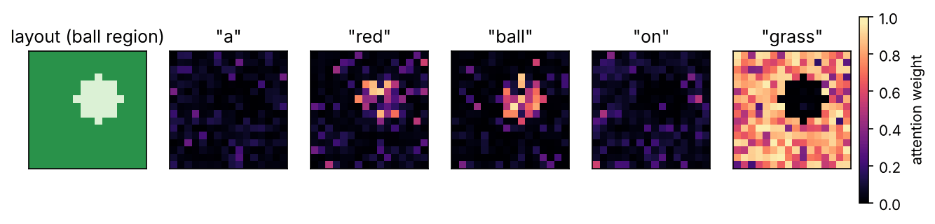
The toy below builds a grid of image features in which a disk region resembles the words “red” and “ball” and the background resembles “grass”, then runs one cross-attention step. The projection matrices are identities to keep it readable; in a trained model they are learned.
Code · Python · 26 lines
import numpy as np

rng = np.random.default_rng(0)
d = 32                                       # feature width
words = ["a", "red", "ball", "on", "grass"]  # the prompt, one text token per word
E = rng.normal(size=(len(words), d))         # text-encoder outputs, one row per word

# A 16 x 16 grid of image tokens: a disk ("the ball") on a background ("the grass").
yy, xx = np.mgrid[:16, :16]
ball = ((yy - 6) ** 2 + (xx - 9) ** 2 <= 9).ravel()   # 29 of the 256 positions
X = 1.0 * rng.normal(size=(256, d))                   # noisy image features
X[ball] += 0.5 * (E[1] + E[2])                        # ball region looks like "red ball"
X[~ball] += 0.5 * E[4]                                # background looks like "grass"

# Cross-attention: queries from the image, keys and values from the text.
# Real models learn W_q, W_k, W_v; identity matrices keep the toy readable.
Q, K, V = X, E, E
scores = Q @ K.T / np.sqrt(d)                         # 256 image tokens x 5 words
A = np.exp(scores - scores.max(axis=1, keepdims=True))
A /= A.sum(axis=1, keepdims=True)                     # softmax over the words
out = A @ V                                           # each image token gets a mix of word values

print("each row sums to 1:", np.allclose(A.sum(axis=1), 1), "| output shape:", out.shape)
for j, w in enumerate(words):
    print(f"{w:6s} mean weight inside the ball={A[ball, j].mean():.2f}  "
          f"outside={A[~ball, j].mean():.2f}")
It prints:
Code · 6 lines
each row sums to 1: True | output shape: (256, 32)
a      mean weight inside the ball=0.02  outside=0.06
red    mean weight inside the ball=0.43  outside=0.07
ball   mean weight inside the ball=0.52  outside=0.04
on     mean weight inside the ball=0.02  outside=0.08
grass  mean weight inside the ball=0.01  outside=0.74
(These numbers come from our toy run, not from any trained model.) Inside the disk, almost all the attention goes to “red” and “ball”; outside, three quarters of it goes to “grass”. The function words “a” and “on” get little weight anywhere. Figure 3 shows the five maps. Notice what the mechanism does not guarantee: “red” and “ball” share the same region because the features say so, and nothing in the attention formula forces a color word to attach to the right object. When two objects are present, a color can attend to the wrong one, which is one root of the attribute-binding failures discussed later [28].
Guidance as used in practice
Classifier-free guidance (CFG) is derived and tested in ML 08; here is the reminder. During training the caption is dropped (replaced by an empty prompt) for a random fraction of examples, so one network learns both a conditional and an unconditional prediction [11]. At sampling time the two are combined, , where and are the predictions with and without the prompt and is the guidance scale; moves past the conditional prediction toward the prompt.
For a system builder, four practical facts matter:
- It is a dial, not a measurement. Higher usually gives more prompt-faithful, higher-contrast images with less variety; very high gives over-saturated, distorted images. Report the value and the convention (some code writes ).
- It doubles the work per step unless the two predictions are batched, so a 30-step guided sampler costs about 60 network evaluations.
- It also works for token models. Autoregressive and masked token generators apply the same formula to next-token logits (ML 09).
- Distilled models may bake it in. Some distilled checkpoints are trained to reproduce guided outputs, so the guidance scale becomes an input or disappears; read the release documentation before comparing settings (ML 08).
Backbones and some landmark systems
The denoiser was first a U-Net [29], a convolutional encoder–decoder with skip connections, with cross-attention layers inserted at several resolutions [5]. The diffusion transformer (DiT) replaces it with a Vision Transformer over latent patches and showed steady gains as transformer compute grew [3] (details in ML 08). Large recent systems mostly use transformers. The table lists a few systems whose design is documented in papers; it is a map of design choices, not a ranking.
| System | Where it generates | Generator and backbone | Text conditioning |
|---|---|---|---|
| Latent diffusion / Stable Diffusion [5] | autoencoder latent | diffusion, U-Net | cross-attention to a text encoder |
| DALL·E 2 [27] | pixels | diffusion decoder from a CLIP image embedding | a prior maps the caption to a CLIP image embedding |
| Imagen [4] | pixels, 64 → 256 → 1024 cascade | diffusion | frozen T5-XXL |
| Parti [30] | discrete tokens (ViT-VQGAN) | autoregressive encoder–decoder transformer | the text is the encoder’s input |
| Muse [31] | discrete tokens | masked parallel decoding, transformer | embeddings from a pretrained language model |
| SDXL [25] | autoencoder latent | diffusion, larger U-Net, optional refiner | two text encoders |
| Stable Diffusion 3 [20] | autoencoder latent | rectified flow, MM-DiT transformer | two CLIP encoders and T5-XXL |
The resolutions of the Imagen cascade are from the project page listed with its reference.
Optional: Stable Diffusion 3 (in the Paper guides). How one paper combines a rectified-flow objective, a joint text–image transformer, three text encoders and curated captions, and how to read its ablations.
Control, personalization and editing
Plain version. A prompt is a weak steering wheel: words cannot pin down an exact pose, a particular person’s dog, or “change only the hat”. Three groups of methods add stronger steering: extra control images (edges, depth, pose), small personalization updates that teach the model a new concept, and editing procedures that change a given image while keeping the rest.
Spatial control: ControlNet
ControlNet adds a spatial condition (an edge map, a depth map, a segmentation, a human pose) to a large pretrained text-to-image model without damaging it [7]. It locks the original network, makes a trainable copy of its encoding layers that receives the condition, and connects the copy back to the original through zero convolutions: convolutions whose weights and biases start at zero. At the first training step the added branch outputs exactly zero, so the model behaves exactly like the original and learning starts from a working generator. The paper reports robust training with both small (under 50k) and large (over 1M) datasets [7].
Optional: ControlNet’s zero convolutions (in the Supplementary notes). The equation of one controlled block and why gradients still reach the zero-initialized layers.
Personalization: teaching the model a new concept
Three methods trade storage, speed and fidelity differently:
- Textual inversion keeps the whole model frozen and learns only a new word embedding (a new “pseudo-word”) from 3–5 images of a concept, by minimizing the usual denoising loss on those images [32]. The stored result is a single vector, but its expressiveness is limited by what the frozen model can already draw.
- DreamBooth fine-tunes the whole model on a few images of a subject captioned with a rare identifier plus the class name, such as “a [V] dog”, and adds a class-specific prior-preservation loss that keeps the model able to draw ordinary dogs; without it, the model drifts and loses diversity [33].
- LoRA (low-rank adaptation) freezes each weight matrix and learns an additive update with , and a small rank [34]. It was introduced for language models; the same update can be attached to the attention layers of a text-to-image denoiser, which makes a personalized style or subject a small file that can be switched on and off (ML 10, PEFT).
Optional: Personalization objectives side by side (in the Supplementary notes). The exact losses of textual inversion and DreamBooth, and what each method stores.
Editing and inpainting
- SDEdit adds noise to an input image (for example a rough color sketch) up to an intermediate noise level, then runs the ordinary reverse process [6]. A low starting noise level keeps the input’s layout and colors (faithful); a high one gives the model more freedom (realistic). One number sets the balance.
- Prompt-to-Prompt edits a generated image by changing the prompt (“a cat on a bike” → “a dog on a bike”) while re-using the original cross-attention maps during sampling, so the layout stays the same and only the changed word’s content changes [8]. Editing a real photo this way first requires finding a noise that reproduces it, for example with deterministic DDIM inversion (ML 08).
- InstructPix2Pix follows written instructions (“make it look like winter”). Its training data was generated automatically by combining a language model (GPT-3) and a text-to-image model (Stable Diffusion) into a large set of before-and-after editing examples; a conditional diffusion model trained on these pairs then edits in a single sampling run, without per-image fine-tuning or inversion [9].
- RePaint inpaints with an unconditional diffusion model: at every reverse step it replaces the known region with a correctly noised copy of the input and lets the model generate only the masked region [10].
A survey by Huang et al. organizes the many diffusion-based editing methods by learning strategy, input condition and task [35].
Fast sampling, briefly
A text-to-image model is used interactively, so the number of network calls matters. The routes are covered in ML 08, few-step generation: deterministic samplers such as DDIM need fewer steps with the same network [36]; progressive distillation halves the step count repeatedly [37]; consistency models learn to jump from any point of a trajectory to its end [38]; and adversarial diffusion distillation (ADD) combines a diffusion teacher with an adversarial loss to sample a large model in 1–4 steps [22]. When you compare systems, count every network evaluation (both guidance passes included) plus the decoder.
Autoregressive and unified multimodal generators
Plain version. An autoregressive generator writes an image the way a language model writes a sentence: one token, or one group of tokens, at a time, each conditioned on what came before. The newest step is to use one transformer for both text and images, so the same model can describe a picture, answer questions about it and draw a new one.
The autoregressive line in one paragraph
The theory is in ML 09; here is the summary. A tokenizer (VQ-VAE or VQGAN, ML 09) turns the image into a grid of integers, and a transformer models them with the chain rule, trained by next-token cross-entropy with teacher forcing (ML 09). Raster-order models such as Parti [30] and LlamaGen [39] predict one token per step; masked models such as MaskGIT [40] and Muse [31] predict many tokens in parallel and refine them over a few rounds (ML 09); VAR predicts a whole, sharper token map per step, coarse to fine [41] (ML 09); and MAR drops the discrete codebook and models each continuous token with a small diffusion head [21] (ML 09). Sampling cost, KV caching and the comparison with diffusion are in ML 09.
Autoregressive text-to-image in practice
From the system side, four facts are worth knowing.
- The text enters as context, not through cross-attention to a separate denoiser. Parti treats text-to-image as translation: a transformer encoder reads the prompt and a decoder writes image tokens; the paper scales this encoder–decoder model to 20 billion parameters and introduces the PartiPrompts benchmark of over 1,600 English prompts [30]. Muse instead feeds a text embedding from a pretrained large language model to a masked token transformer, and it supports inpainting, outpainting and mask-free editing without fine-tuning [31].
- Language-model infrastructure transfers. LlamaGen uses a plain Llama-style decoder; besides class-conditional models from 111M to 3.1B parameters it trains a 775M text-conditional model, and it reports that an LLM serving framework sped up image generation by 326%–414% [39].
- The tokenizer is decisive. MAGVIT-v2 argues that the tokenizer is the key component: with its new “lookup-free” quantizer, which lets the vocabulary grow large, a language model outperformed diffusion models on ImageNet when given the same training data, a similar model size and a similar training budget [42]. Small details such as text and thin lines are typical casualties of a coarse tokenizer (ML 09).
- Guidance and sampling knobs carry over. CFG on logits, temperature and top- sampling set the fidelity–diversity balance, and every guided step costs two forward passes.
Unified multimodal models
Plain version. Instead of a text model that hands a prompt to a separate image model, a unified model puts text and image pieces into one sequence and trains one transformer on it. The design questions are: are image pieces discrete tokens or continuous vectors, is the image part generated by next-token prediction or by diffusion, and do understanding and generation share one image encoder?
The models below are documented in papers and illustrate the main design choices:
- Chameleon puts discrete image tokens and text tokens in one sequence from the start (“early fusion”) and handles captioning, question answering and the generation of text, images and mixed documents with one model [43].
- Emu3 trains one transformer from scratch with next-token prediction only, over discrete tokens of images, text and video [44].
- Transfusion keeps images continuous and trains one transformer with a next-token loss on text and a diffusion loss on image patches; its authors report that this scales better than quantizing images into tokens [45].
- Show-o combines autoregressive text modeling with discrete (masked) diffusion over image tokens [46].
- Janus shares one transformer but uses separate visual encoders for understanding and for generation, because the two tasks need different levels of image detail [47].
| Model | Image representation | Image objective | Visual encoders |
|---|---|---|---|
| Chameleon [43] | discrete tokens | next token | one, shared |
| Emu3 [44] | discrete tokens | next token | one, shared |
| Transfusion [45] | continuous patches | diffusion | one, shared |
| Show-o [46] | discrete tokens | masked (discrete) diffusion | one, shared |
| Janus [47] | discrete tokens for generation | next token | separate for understanding and generation |
Optional: Unified multimodal models, one by one (in the Supplementary notes). What each paper changes in the transformer, the tokenizer and the training data.
What is still open: whether one model can be state-of-the-art at both understanding and generation at the same size, how much a shared visual tokenizer costs each task (the motivation for Janus), and how evaluation should compare a unified model with a specialized diffusion system. Claims about scaling in these papers are each paper’s own measurements, on its own data; they are not yet a settled law.
Evaluating text-to-image models
Plain version. You need four kinds of evidence: do the images look real and varied (distribution metrics), do they match their prompts overall (alignment scores), do they get the details right (compositional checks), and do people like them (human preference). Each kind catches failures the others miss.
Distribution metrics and their pitfalls
FID compares feature statistics of generated and real images; precision and recall separate fidelity from coverage. Both are defined and implemented in ML 07, and ML 08 covers the newer feature spaces. For text-to-image models the common protocol is a zero-shot COCO FID: generate images from COCO captions [48] with a model that was not trained on COCO and compare with the real COCO images, as Imagen did [4]. Five pitfalls matter in practice:
- Finite-sample bias. FID is biased for finite sample sets, and the bias depends on the model being evaluated, so even equal sample counts do not make a comparison fully fair; Chong and Forsyth propose extrapolating to an infinite sample count [49].
- Preprocessing. The resizing filter and JPEG compression used before feature extraction change FID substantially; Parmar et al. show this and provide a reference implementation [50].
- What the features see. Inception features are so close to ImageNet classes that matching the class histogram of generated images can lower FID without making images better [51].
- Agreement with people. In a large human study no common metric correlated strongly with human judgments, and FID under-rated diffusion models; the authors recommend richer feature extractors such as DINOv2 [52]. CMMD replaces Inception features and the Gaussian assumption with CLIP embeddings and a kernel distance [53].
- No alignment. FID does not look at the prompt at all: a model that ignores every prompt but draws beautiful COCO-like images can score well.
Prompt alignment: CLIPScore
CLIPScore measures how well an image and a text agree in CLIP’s embedding space [54]. With the CLIP embedding of the text and the CLIP embedding of the image,
where is the cosine similarity and is a constant that only rescales the range ( in the original paper, which proposed the score for image captioning). For text-to-image evaluation the score is averaged over prompt–image pairs. It is cheap and needs no reference image, but it inherits CLIP’s blind spots: an embedding that summarizes the whole image is weak at counts, spatial relations and which attribute belongs to which object. The GenEval study found that its object-level checks agree with human judgments much better than CLIPScore on such compositional tasks [55].
Compositional benchmarks
Plain version. Instead of one overall similarity, ask concrete yes-or-no questions about the image: is there a dog, are there exactly three, is the dog left of the cat, is the car red? A detector or a vision–language model answers them.
GenEval generates prompts from templates for six tasks (single object, two objects, counting, colors, position and attribute binding), detects the objects with an instance-segmentation model, classifies object colors with CLIP, and scores each image as correct or not [55]. T2I-CompBench provides 6,000 compositional prompts in three categories (attribute binding, object relationships and complex compositions) with metrics tailored to each [56]. Imagen’s DrawBench [4] and Parti’s PartiPrompts [30] are prompt sets for side-by-side human comparison. Object detection itself is the subject of DLCV 03; an open-vocabulary detector (DLCV 03) can check objects outside a fixed class list.
Optional: GenEval (in the Paper guides). How the benchmark is built, how its scores are computed and how to read its tables.
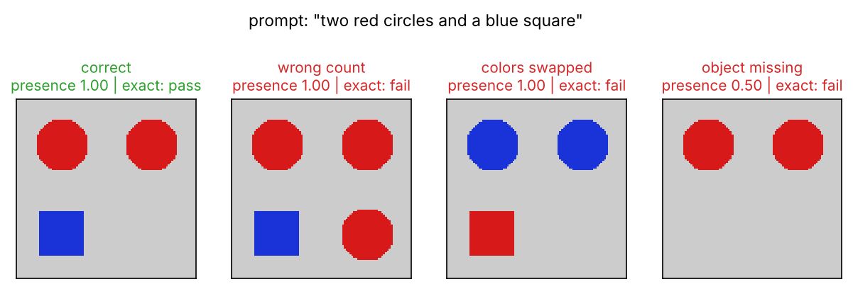
The toy below shows why object-level checks matter. It draws synthetic “generated images” made of colored disks and squares for the prompt “two red circles and a blue square”, detects the shapes with connected components, and compares two scores: a presence score that asks which prompt words appear anywhere in the image (a deliberately simple stand-in for a global similarity score, not CLIP itself) and an exact check that requires every (color, shape) pair with the right count, as GenEval does.
Code · Python · 49 lines
import numpy as np
from skimage.draw import disk, rectangle
from skimage.measure import label, regionprops

COLORS = {"red": (0.85, 0.1, 0.1), "blue": (0.1, 0.2, 0.85)}

def render(objects, size=96):
    """Draw (color, shape) objects at fixed slots on a gray canvas: a stand-in for a generated image."""
    img = np.full((size, size, 3), 0.8)
    for k, (col, shape) in enumerate(objects):
        cy, cx = 24 + 48 * (k // 2), 24 + 48 * (k % 2)
        if shape == "circle":
            rr, cc = disk((cy, cx), 14)
        else:
            rr, cc = rectangle((cy - 12, cx - 12), extent=(24, 24))
        img[rr, cc] = COLORS[col]
    return img

def detect(img):
    """Toy 'detector': connected colored regions -> (color, shape) pairs."""
    found = []
    for region in regionprops(label(np.abs(img - 0.8).sum(-1) > 0.3)):
        r, g, b = img[tuple(region.coords.T)].mean(0)
        col = "red" if r > b else "blue"
        shape = "square" if region.extent > 0.9 else "circle"   # filled bbox fraction
        found.append((col, shape))
    return found

def presence_score(prompt, img):
    """Bag-of-words check: which prompt words appear anywhere (ignores counts and binding)."""
    words = {w for obj in prompt for w in obj}
    seen = {w for obj in detect(img) for w in obj}
    return len(words & seen) / len(words)

def exact_check(prompt, img):
    """GenEval-style check: every (color, shape) pair with the right count."""
    return sorted(detect(img)) == sorted(prompt)

prompt = [("red", "circle"), ("red", "circle"), ("blue", "square")]   # "two red circles and a blue square"
candidates = {
    "correct":          prompt,
    "wrong count":      prompt + [("red", "circle")],
    "colors swapped":   [("blue", "circle"), ("blue", "circle"), ("red", "square")],
    "object missing":   prompt[:2],
}
for name, objs in candidates.items():
    img = render(objs)
    print(f"{name:15s} presence score={presence_score(prompt, img):.2f}  "
          f"exact check={'pass' if exact_check(prompt, img) else 'fail'}")
It prints:
Code · 4 lines
correct         presence score=1.00  exact check=pass
wrong count     presence score=1.00  exact check=fail
colors swapped  presence score=1.00  exact check=fail
object missing  presence score=0.50  exact check=fail
The presence score gives full marks to the wrong count and to the swapped colors, because every word of the prompt is present somewhere; only the exact check catches them. Real benchmarks replace our connected-component “detector” with a trained detector and a color classifier, and inherit their errors: the check is only as good as the detector, which is why GenEval reports its agreement with human annotators [55]. Figure 4 shows the four images.
Human preference and holistic evaluation
People remain the reference. Because human studies are slow, several groups trained preference models that predict which of two images people prefer for a prompt: ImageReward was trained on 137k expert comparisons [57], and PickScore on Pick-a-Pic, an open dataset of real users’ choices collected through a web app [58]. HEIM evaluates models along 12 aspects (including alignment, quality, aesthetics, originality, reasoning, knowledge, bias, toxicity, fairness, robustness, multilinguality and efficiency) over 62 scenarios and 26 models, and finds that no single model is best at everything [59]. A learned preference model is itself a model with biases; if a generator is tuned to maximize it, the score can rise faster than real quality.
A reporting checklist. For any claim about a text-to-image model, state: the prompts (and how they were sampled), the number of images per prompt and seeds, the sampler, the number of steps and guidance scale, the resolution, the metric implementations and feature extractors, and show uncurated samples. Report distribution, alignment, compositional and preference results side by side, and say which numbers you ran yourself and which were copied from papers.
Data
Plain version. A generator can only learn what its training images and captions show, so the dataset decides its knowledge, its style and many of its biases. Large text-to-image datasets are scraped from the web, which raises questions of quality, copyright and consent.
- Class-conditional benchmarks use ImageNet [60]; text-to-image papers often evaluate zero-shot on COCO captions [48]; face generators use datasets such as FFHQ, the high-quality face dataset introduced with StyleGAN [1].
- LAION-5B is an openly released dataset of 5.85 billion CLIP-filtered image–text pairs, of which 2.32 billion have English text [61]. It distributes URLs and alt-text rather than the images themselves, and its datasheet states that LAION releases the metadata under CC-BY-4.0 but does not own the copyright of the images or text, that people depicted in the images may not have consented to their upload, and that the dataset should be used for academic research in its current form; it describes ways to request removal of links [61].
- Content audits. Birhane et al. examined the earlier LAION-400M dataset and found explicit and problematic image–text pairs, including pornography, malign stereotypes and slurs [62].
- Captions are data too. Stable Diffusion 3 trains on a 50/50 mix of original captions and synthetic captions written by a vision–language model, and filters its data for sexual content, low aesthetic scores and near-duplicates (to reduce regurgitation of training images) [20].
Risks and responsible use
Plain version. A model that can draw anything can also copy, stereotype and deceive. The practical responses are to measure these behaviors, to reduce them in the data and the model, and to label generated images so that viewers can check where they came from.
Memorization and copying
Carlini et al. showed that diffusion models memorize individual training images and can emit them: with a generate-and-filter pipeline they extracted over a thousand training examples, from photos of individual people to trademarked logos, and they found diffusion models less private than GANs in their experiments [63]. Somepalli et al. built image-retrieval tools to compare generated images with training images and found cases where models, including Stable Diffusion, copied content from their training data [64]. Deduplicating training data [20] and checking generated images against the training set are the standard first defenses.
Bias
Bianchi et al. found that ordinary prompts (traits, occupations, objects) produce and amplify demographic stereotypes, and that neither counter-stereotypical prompts nor system guardrails removed them in their tests [65]. Luccioni et al. proposed a way to measure social bias in generated people by comparing the variation caused by gender and ethnicity words with the variation caused by professions, and found under-representation of marginalized identities in the three systems they tested [66]. Bias evaluation needs its own prompts and analysis; overall quality metrics do not reveal it. See also ML 10, data provenance, bias and privacy.
Deepfakes, provenance and watermarks
Two complementary tools exist for labeling generated images:
- Signed provenance (C2PA). The C2PA specification defines a “manifest” of provenance claims (who made the asset and how) that is cryptographically signed and bound to the asset, either by a cryptographic hash (a hard binding) or by a fingerprint or invisible watermark (a soft binding) [67]. A valid signature shows that the claims were not altered; it does not prove that the content is true, and a manifest stored in metadata can simply be removed.
- Invisible watermarks. Tree-Ring watermarking hides a pattern in the Fourier transform of the initial noise of a diffusion sampler and detects it by inverting the sampler [68]. Stable Signature fine-tunes the latent decoder so that every generated image carries a binary signature that a pretrained extractor can read [69]. Classical watermarking is covered in IP 08.
Neither is a complete answer. Zhao et al. prove and show that pixel-level invisible watermarks can be removed by a “regeneration attack” (add noise, then reconstruct with a generative model) [70], and Saberi et al. show a fundamental trade-off for low-perturbation watermarks between failing to detect watermarked images and falsely flagging real ones, and demonstrate spoofing attacks that make real images look watermarked [71]. Treat provenance and watermarks as evidence to weigh, not as proof.
Optional: Hard bindings, soft bindings and watermarks (in the Supplementary notes). How each mechanism survives cropping, re-encoding and metadata stripping.
Failure modes
Plain version. Today’s generators are excellent at “a photo of X” and still unreliable at the precise parts of a request: how many, which one has which color, where things are, what the text says. Knowing the typical failures tells you what to test.
- Counting. “Four apples” often gives three or five. GenEval’s counting task (2, 3 or 4 objects) measures it directly [55].
- Spatial relations. “A cup to the left of a laptop” is often drawn in the wrong arrangement; in GenEval’s original study the best model produced the correct position in only 15% of images [55].
- Attribute binding and leakage. In “a red car and a blue bench” the colors can swap between objects or leak onto the background; GenEval’s best model at the time got attribute binding right in 35% of images [55]. Attend-and-Excite also documents catastrophic neglect, where one of the subjects in the prompt is not drawn at all, and steers the cross-attention maps at sampling time so that every subject token gets attention [28].
- Text rendering. Misspelled signs and labels are common; character-blind text encoders are one documented cause [26], and Stable Diffusion 3’s ablation shows that the T5 encoder matters most for prompts with written text [20].
- Hands. Generated hands often have the wrong number of fingers or irregular shapes; HandRefiner repairs them afterwards by inpainting conditioned on a reconstructed hand mesh [72]. Note that object-level benchmarks cannot check this: GenEval’s authors point out that their detector can count people but not fingers [55].
- Copying of content and style. A prompt that names a famous image, product or artist can pull out a near-copy of training content [64], [63].
How to test. Build a small prompt set per failure type, generate several images per prompt with fixed seeds, check them with an object-level tool where possible and by eye where not, and track the failure rate across model versions.
Modern view
Surveys worth reading.
- Zhang et al. [73] (2023) is a self-contained review of text-to-image diffusion models: a short introduction to diffusion, the background of text-conditioned synthesis, the pioneering systems and their improvements, applications beyond images (video, other modalities, text-guided editing) and open challenges.
- Croitoru et al. [74] (IEEE TPAMI 2023) survey diffusion models in vision, grouped by formulation (DDPM, score networks, SDEs) and by application (generation, super-resolution, inpainting, editing, translation, segmentation).
- Huang et al. [35] (IEEE TPAMI 2025) classify diffusion-based image editing by learning strategy, user-input condition and editing task, give special attention to inpainting and outpainting, and propose a benchmark (EditEval) with a metric scored by a large multimodal model.
- Xiong et al. [75] (TMLR 2025) survey autoregressive vision models, split by representation into pixel-based, token-based and scale-based models, and discuss their links to other generative families and their uses in image, video, 3-D and multimodal generation.
State of the art, 2023–2026. (1) Latent transformers with flow objectives and several text encoders became the standard large-scale recipe, as in Stable Diffusion 3 [20], building on DiT [3]. (2) Autoregressive models returned through better tokenizers [42], next-scale prediction [41] and continuous tokens [21]. (3) Unified multimodal models that understand and generate with one transformer appeared in quick succession [43], [45], [46], [47], [44]. (4) Few-step generation made interactive use practical [22], [38]. (5) Evaluation moved beyond FID toward compositional checks [55], [56], learned preference models [57], [58] and holistic benchmarks [59]. Recent work also revisits pixel-space generation and generation in representation spaces; see ML 08, pixel space, latent space and representation autoencoders.
Open problems. Reliable counting, spatial reasoning and attribute binding; legible text in any language; evaluation metrics that agree with people at the level of single images and cannot be gamed; preventing memorization without losing quality; measuring and reducing bias; provenance that survives editing; consent and licensing for training data; and the cost of high-resolution and video generation.
Optional: Latent Diffusion, SD3 (in the Paper guides). Read the latent representation first, then how SD3 changes the training path and multimodal transformer.
Key takeaways
- Define the condition and output constraints before choosing a generator.
- Generator objectives and image representations are separate choices; systems can combine families.
- Inspect how text or spatial conditions enter the model, and what guidance changes at inference.
- Attention maps show internal interactions, not a guarantee of correct object–attribute binding.
- Control, personalization and editing impose different data and compute requirements.
- Combine distribution, alignment, composition and human-preference evaluations; report the sampling protocol and cost.
- Inspect memorization, bias and provenance separately from visual quality.
Exercises
- Map the tasks. For each task in the table of six kinds of generation, write down what the condition is as a tensor (shape and type) for a latent text-to-image model, and which part of the pipeline in Figure 2 receives it.
Hint
The prompt becomes token embeddings that enter through cross-attention. A class label can be written as a text prompt or as an embedding added to the time embedding. For image-to-image and editing, the input image is encoded to a latent and either noised to an intermediate level (SDEdit) or concatenated to the denoiser’s input channels (InstructPix2Pix); a control image enters through ControlNet’s trainable copy; a mask for inpainting decides which latent positions are regenerated.
- Neglect in the toy. In the cross-attention snippet, add a sixth word “dog” whose embedding is a fresh random vector that no image region resembles. What does its attention map look like, and what does it do to the weights of the other words? Then make the ball region resemble only “ball” (not “red”). Which map changes?
Hint
The “dog” column gets small, unstructured weights everywhere, because no query matches its key: nothing tells the generator where a dog should go, which is the situation Attend-and-Excite fixes by strengthening a neglected token’s attention during sampling. The softmax still sums to one per row, so the other words lose a little weight. Removing “red” from the ball features makes the “red” map dark: a color word attends only where the features already suggest it.
- Break the metric. Extend the compositional-check snippet with a candidate that has the right objects but in an image where the blue square overlaps one red circle. What does the toy detector report, and what would a real detector-based benchmark need to handle it?
Hint
Overlapping shapes merge into one connected component, so the toy detector sees fewer objects and the wrong shape; the exact check fails even though a person might accept the image. Real benchmarks use instance segmentation, which can separate overlapping objects, and GenEval adds rules for overlapping boxes when judging positions. Every automatic check has such blind spots, which is why benchmarks report agreement with human annotators.
- Design an evaluation. You must decide whether a new model is better than the current one at “product photos with a short brand name on the package”. Write an evaluation plan: prompts, number of images, automatic metrics, human study, and what result would change your decision.
Hint
Use a fixed prompt set that varies product type, text length and background; several seeds per prompt; an OCR check of the rendered text against the requested string; an object-level check of the product type; FID or CMMD against real product photos for realism (with a fixed implementation and sample count); and a blind side-by-side human comparison on alignment and quality. Decide in advance which difference you would act on, and include a memorization check against the training set for brand logos.
- Provenance under editing. An image carries a C2PA manifest with a hard binding and was generated by a model with a Stable Signature watermark. It is then cropped, re-saved as JPEG and uploaded to a site that strips metadata. Which evidence of its origin is likely to survive, and why?
Hint
The manifest is lost with the metadata, and even if it were kept, the hash of the hard binding would no longer match the cropped, re-encoded pixels. A soft binding or a robust invisible watermark can survive moderate cropping and compression (Stable Signature reports detection after strong cropping), but a regeneration attack can remove pixel-level watermarks. The honest answer is “maybe the watermark, not the manifest”, which is why the two are designed to work together.
References
- T. Karras, S. Laine and T. Aila, “A Style-Based Generator Architecture for Generative Adversarial Networks,” CVPR, 2019. arXiv
- A. Brock, J. Donahue and K. Simonyan, “Large Scale GAN Training for High Fidelity Natural Image Synthesis,” ICLR, 2019. arXiv
- W. Peebles and S. Xie, “Scalable Diffusion Models with Transformers,” ICCV, 2023. CVF
- C. Saharia, W. Chan, S. Saxena et al., “Photorealistic Text-to-Image Diffusion Models with Deep Language Understanding,” NeurIPS, 2022. arXiv · project page
- R. Rombach, A. Blattmann, D. Lorenz, P. Esser and B. Ommer, “High-Resolution Image Synthesis with Latent Diffusion Models,” CVPR, 2022. CVF
- C. Meng, Y. He, Y. Song et al., “SDEdit: Guided Image Synthesis and Editing with Stochastic Differential Equations,” ICLR, 2022. arXiv
- L. Zhang, A. Rao and M. Agrawala, “Adding Conditional Control to Text-to-Image Diffusion Models,” ICCV, 2023. CVF
- A. Hertz, R. Mokady, J. Tenenbaum et al., “Prompt-to-Prompt Image Editing with Cross-Attention Control,” ICLR, 2023. arXiv
- T. Brooks, A. Holynski and A. A. Efros, “InstructPix2Pix: Learning to Follow Image Editing Instructions,” CVPR, 2023. CVF
- A. Lugmayr, M. Danelljan, A. Romero et al., “RePaint: Inpainting using Denoising Diffusion Probabilistic Models,” CVPR, 2022. CVF
- J. Ho and T. Salimans, “Classifier-Free Diffusion Guidance,” NeurIPS 2021 Workshop on Deep Generative Models and Downstream Applications; arXiv:2207.12598, 2022. arXiv
- I. J. Goodfellow, J. Pouget-Abadie, M. Mirza et al., “Generative Adversarial Nets,” NeurIPS, 2014. arXiv
- D. P. Kingma and M. Welling, “Auto-Encoding Variational Bayes,” ICLR, 2014. arXiv
- A. van den Oord, O. Vinyals and K. Kavukcuoglu, “Neural Discrete Representation Learning,” NeurIPS, 2017. arXiv
- P. Esser, R. Rombach and B. Ommer, “Taming Transformers for High-Resolution Image Synthesis,” CVPR, 2021. CVF
- J. Ho, A. Jain and P. Abbeel, “Denoising Diffusion Probabilistic Models,” NeurIPS, 2020. arXiv
- P. Dhariwal and A. Nichol, “Diffusion Models Beat GANs on Image Synthesis,” NeurIPS, 2021. arXiv
- Y. Lipman, R. T. Q. Chen, H. Ben-Hamu, M. Nickel and M. Le, “Flow Matching for Generative Modeling,” ICLR, 2023. arXiv
- X. Liu, C. Gong and Q. Liu, “Flow Straight and Fast: Learning to Generate and Transfer Data with Rectified Flow,” ICLR, 2023. arXiv
- P. Esser, S. Kulal, A. Blattmann et al., “Scaling Rectified Flow Transformers for High-Resolution Image Synthesis,” ICML, PMLR 235, 2024. arXiv
- T. Li, Y. Tian, H. Li, M. Deng and K. He, “Autoregressive Image Generation without Vector Quantization,” NeurIPS, 2024. arXiv
- A. Sauer, D. Lorenz, A. Blattmann and R. Rombach, “Adversarial Diffusion Distillation,” ECCV, LNCS, pp. 87–103, 2024. doi · arXiv
- A. Radford, J. W. Kim, C. Hallacy et al., “Learning Transferable Visual Models From Natural Language Supervision,” ICML, PMLR 139, 2021. arXiv
- C. Raffel, N. Shazeer, A. Roberts et al., “Exploring the Limits of Transfer Learning with a Unified Text-to-Text Transformer,” Journal of Machine Learning Research, vol. 21, 2020. arXiv
- D. Podell, Z. English, K. Lacey et al., “SDXL: Improving Latent Diffusion Models for High-Resolution Image Synthesis,” ICLR, 2024. arXiv
- R. Liu, D. Garrette, C. Saharia et al., “Character-Aware Models Improve Visual Text Rendering,” ACL, 2023. ACL Anthology
- A. Ramesh, P. Dhariwal, A. Nichol, C. Chu and M. Chen, “Hierarchical Text-Conditional Image Generation with CLIP Latents,” arXiv:2204.06125, 2022. arXiv
- H. Chefer, Y. Alaluf, Y. Vinker, L. Wolf and D. Cohen-Or, “Attend-and-Excite: Attention-Based Semantic Guidance for Text-to-Image Diffusion Models,” ACM Transactions on Graphics, vol. 42, no. 4 (SIGGRAPH), 2023. doi · arXiv
- O. Ronneberger, P. Fischer and T. Brox, “U-Net: Convolutional Networks for Biomedical Image Segmentation,” MICCAI, 2015. arXiv
- J. Yu, Y. Xu, J. Y. Koh et al., “Scaling Autoregressive Models for Content-Rich Text-to-Image Generation,” Transactions on Machine Learning Research, 2022. arXiv
- H. Chang, H. Zhang, J. Barber et al., “Muse: Text-To-Image Generation via Masked Generative Transformers,” ICML, PMLR 202, 2023. arXiv
- R. Gal, Y. Alaluf, Y. Atzmon et al., “An Image is Worth One Word: Personalizing Text-to-Image Generation using Textual Inversion,” ICLR, 2023. arXiv
- N. Ruiz, Y. Li, V. Jampani, Y. Pritch, M. Rubinstein and K. Aberman, “DreamBooth: Fine Tuning Text-to-Image Diffusion Models for Subject-Driven Generation,” CVPR, 2023. CVF
- E. J. Hu, Y. Shen, P. Wallis et al., “LoRA: Low-Rank Adaptation of Large Language Models,” ICLR, 2022. arXiv
- Y. Huang, J. Huang, Y. Liu et al., “Diffusion Model-Based Image Editing: A Survey,” IEEE Transactions on Pattern Analysis and Machine Intelligence, 2025. doi · arXiv
- J. Song, C. Meng and S. Ermon, “Denoising Diffusion Implicit Models,” ICLR, 2021. arXiv
- T. Salimans and J. Ho, “Progressive Distillation for Fast Sampling of Diffusion Models,” ICLR, 2022. arXiv
- Y. Song, P. Dhariwal, M. Chen and I. Sutskever, “Consistency Models,” ICML, PMLR 202, 2023. arXiv
- P. Sun, Y. Jiang, S. Chen et al., “Autoregressive Model Beats Diffusion: Llama for Scalable Image Generation,” arXiv:2406.06525, 2024. arXiv
- H. Chang, H. Zhang, L. Jiang, C. Liu and W. T. Freeman, “MaskGIT: Masked Generative Image Transformer,” CVPR, 2022. CVF
- K. Tian, Y. Jiang, Z. Yuan, B. Peng and L. Wang, “Visual Autoregressive Modeling: Scalable Image Generation via Next-Scale Prediction,” NeurIPS, 2024. arXiv
- L. Yu, J. Lezama, N. B. Gundavarapu et al., “Language Model Beats Diffusion — Tokenizer is Key to Visual Generation,” ICLR, 2024. arXiv
- Chameleon Team, “Chameleon: Mixed-Modal Early-Fusion Foundation Models,” arXiv:2405.09818, 2024. arXiv
- X. Wang, Y. Cui, J. Wang et al., “Multimodal learning with next-token prediction for large multimodal models,” Nature, vol. 650, pp. 327–333, 2026 (preprint “Emu3: Next-Token Prediction is All You Need,” 2024). doi · arXiv
- C. Zhou, L. Yu, A. Babu et al., “Transfusion: Predict the Next Token and Diffuse Images with One Multi-Modal Model,” ICLR, 2025. arXiv
- J. Xie, W. Mao, Z. Bai et al., “Show-o: One Single Transformer to Unify Multimodal Understanding and Generation,” ICLR, 2025. arXiv
- C. Wu, X. Chen, Z. Wu et al., “Janus: Decoupling Visual Encoding for Unified Multimodal Understanding and Generation,” CVPR, 2025. CVF
- T.-Y. Lin, M. Maire, S. Belongie et al., “Microsoft COCO: Common Objects in Context,” ECCV, 2014. arXiv
- M. J. Chong and D. Forsyth, “Effectively Unbiased FID and Inception Score and Where to Find Them,” CVPR, 2020. arXiv
- G. Parmar, R. Zhang and J.-Y. Zhu, “On Aliased Resizing and Surprising Subtleties in GAN Evaluation,” CVPR, 2022. CVF
- T. Kynkäänniemi, T. Karras, M. Aittala, T. Aila and J. Lehtinen, “The Role of ImageNet Classes in Fréchet Inception Distance,” ICLR, 2023. arXiv
- G. Stein, J. C. Cresswell, R. Hosseinzadeh et al., “Exposing Flaws of Generative Model Evaluation Metrics and Their Unfair Treatment of Diffusion Models,” NeurIPS, 2023. arXiv
- S. Jayasumana, S. Ramalingam, A. Veit, D. Glasner, A. Chakrabarti and S. Kumar, “Rethinking FID: Towards a Better Evaluation Metric for Image Generation,” CVPR, 2024. CVF
- J. Hessel, A. Holtzman, M. Forbes, R. Le Bras and Y. Choi, “CLIPScore: A Reference-free Evaluation Metric for Image Captioning,” EMNLP, 2021. ACL Anthology
- D. Ghosh, H. Hajishirzi and L. Schmidt, “GenEval: An Object-Focused Framework for Evaluating Text-to-Image Alignment,” NeurIPS Datasets and Benchmarks Track, 2023. arXiv
- K. Huang, K. Sun, E. Xie, Z. Li and X. Liu, “T2I-CompBench: A Comprehensive Benchmark for Open-world Compositional Text-to-image Generation,” NeurIPS Datasets and Benchmarks Track, 2023. proceedings
- J. Xu, X. Liu, Y. Wu et al., “ImageReward: Learning and Evaluating Human Preferences for Text-to-Image Generation,” NeurIPS, 2023. arXiv
- Y. Kirstain, A. Polyak, U. Singer et al., “Pick-a-Pic: An Open Dataset of User Preferences for Text-to-Image Generation,” NeurIPS, 2023. arXiv
- T. Lee, M. Yasunaga, C. Meng et al., “Holistic Evaluation of Text-To-Image Models,” NeurIPS Datasets and Benchmarks Track, 2023. arXiv
- J. Deng, W. Dong, R. Socher, L.-J. Li, K. Li and L. Fei-Fei, “ImageNet: A Large-Scale Hierarchical Image Database,” CVPR, 2009. doi
- C. Schuhmann, R. Beaumont, R. Vencu et al., “LAION-5B: An Open Large-Scale Dataset for Training Next Generation Image-Text Models,” NeurIPS Datasets and Benchmarks Track, 2022. arXiv
- A. Birhane, V. U. Prabhu and E. Kahembwe, “Multimodal datasets: misogyny, pornography, and malignant stereotypes,” arXiv:2110.01963, 2021. arXiv
- N. Carlini, J. Hayes, M. Nasr et al., “Extracting Training Data from Diffusion Models,” USENIX Security Symposium, 2023. USENIX · arXiv
- G. Somepalli, V. Singla, M. Goldblum, J. Geiping and T. Goldstein, “Diffusion Art or Digital Forgery? Investigating Data Replication in Diffusion Models,” CVPR, 2023. CVF
- F. Bianchi, P. Kalluri, E. Durmus et al., “Easily Accessible Text-to-Image Generation Amplifies Demographic Stereotypes at Large Scale,” ACM FAccT, 2023. doi
- A. S. Luccioni, C. Akiki, M. Mitchell and Y. Jernite, “Stable Bias: Analyzing Societal Representations in Diffusion Models,” NeurIPS Datasets and Benchmarks Track, 2023. arXiv
- Coalition for Content Provenance and Authenticity (C2PA), “C2PA Technical Specification,” version 2.1, 2024. specification
- Y. Wen, J. Kirchenbauer, J. Geiping and T. Goldstein, “Tree-Ring Watermarks: Fingerprints for Diffusion Images that are Invisible and Robust,” NeurIPS, 2023. arXiv
- P. Fernandez, G. Couairon, H. Jégou, M. Douze and T. Furon, “The Stable Signature: Rooting Watermarks in Latent Diffusion Models,” ICCV, 2023. CVF
- X. Zhao, K. Zhang, Z. Su et al., “Invisible Image Watermarks Are Provably Removable Using Generative AI,” NeurIPS, 2024. arXiv
- M. Saberi, V. S. Sadasivan, K. Rezaei et al., “Robustness of AI-Image Detectors: Fundamental Limits and Practical Attacks,” ICLR, 2024. arXiv
- W. Lu, Y. Xu, J. Zhang, C. Wang and D. Tao, “HandRefiner: Refining Malformed Hands in Generated Images by Diffusion-based Conditional Inpainting,” ACM Multimedia, 2024, pp. 7085–7093. doi
- C. Zhang, C. Zhang, M. Zhang, I. S. Kweon and J. Kim, “Text-to-image Diffusion Models in Generative AI: A Survey,” arXiv:2303.07909, 2023. arXiv
- F.-A. Croitoru, V. Hondru, R. T. Ionescu and M. Shah, “Diffusion Models in Vision: A Survey,” IEEE Transactions on Pattern Analysis and Machine Intelligence, 2023. doi
- J. Xiong, G. Liu, L. Huang et al., “Autoregressive Models in Vision: A Survey,” Transactions on Machine Learning Research, 2025. arXiv
Check your understanding
This tutorial has 5 exercises. Can you solve them without opening the hints?
Go to the exercises ↑Next DLCV 12A · Video Generation · 41 min